Simplified bidimensional water temperature modelling during spring time on the St-Lawrence river.

SIMPLIFIED BIDIMENSIONAL WATER

TEMPERATURE MODELLING

DURING SPRING TIME

ON THE ST-LAWRENCE RIVER

JEAN MORIN, OLIVIER CHAMPOUX AND YVES SECRETAN

Morin, J., O. Champoux and Y. Secretan, 2004. Simplified bidimensional water temperature modelling durin spring time on the St-Lawrence River. Rapport INRS-ETE N° R-773. Technical Report RT-136, Meteorological Service of Canada, Environment Canada, Sainte-Foy. 36 p.

INDEX

INDEX ... iii

LIST OF FIGURES ... v

LISTE OF TABLES ... vii

RESEARCH TEAM ... IX 1. INTRODUCTION ... 1

2. METHODOLOGY ... 3

2.1 OVERVIEW OF THE METHODOLOGY ... 3

2.1.1 Historical reconstruction of meteorological data ... 4

2.1.2 Temperature for tributaries and injlows ... 5

2.2 2D TEMPERATURE MODEL: STRUCTURE AND USE ... 6

2.2.1 Hydrology and numericalfield model.. ... ... 6

2.2.2 Hydrodynamic model ... 6

2.2.3 Water temperature model ... ... 6

2.2.4 Mathematical model ... ... 7

2.2.4.1 Numerical implementation ... 8

3. RESULTS ... 11

3.1 SYNTHETIC CUMA TIC SERIES FOR THE ST. LAWRENCE RIVER; COMPLETION OF CUMA TIC DATA AT DORVAL STATION ... 11

3.1.1 Cloud cover ... 11 3.1.2 Relative humidity ... 11 3.1.3 Atmospheric pressure ... 12 3.1.4 Air temperature ... 13 3.1.5 Solar radiation ... 14 3.1. 6 Precipitation ... 16 3.1.7 Wind velocity ... 17

3.2 TEMPERATURE BOUNDARY CONDITIONS FOR THE TRIBUTARIES AND MAIN INFLOW ... 17

3.2.1 Ottawa River (Carillon Dam) ... 17

3.2.2 Des Milles-Iles and des Prairies Rivers ... 18

3.2.3 L'Assomption River ... 18 3.2.4 Richelieu River ... 19 3.2.5 Yamaska River ... 20 3.2.6 Saint-François River ... 20 3.2.7 Nicolet River ... ... 21 3.2.8 DuLoup River ... 21 3.2.9 Maskinongé River ... ... 22

3.2.10 St. Lawrence River at Beauharnois Dam ... 22

3.3.1 Global meteorological modeling conditions (QM aggregation) ... 23

3.3.2 Tributaries water temperature boundary conditions (QM aggregation) ... 23

3.3.2.1 Quarter-monthly water temperature simulations ... 24

3.4 CALIBRA TI ON OF DIFFUSIVITY IN THE 2D TEMPERATURE MODEL ... 29

3.4.1 Lake Saint-Louis calibration ... ... 29

3.4.2 Lake Saint-Pierre calibration. ... 30

3.5 LAKE SAINT-PIERRE WATER TEMPERATURE DURING FISH SPAWNING PERIODS ... 31

4. CONCLUSION ... 33

LIST OF FIGURES

FIGURE 1: LOCA TION OF TEMPERATURE MEASUREMENT STATIONS ASSOCIATED WITH MAIN

TRIBUTARIES ... 5

FIGURE 2: COMPLETE SERIES OF THE DAILY CLOUD COVER FOR DORVAL STATION ... 11

FIGURE 3: COMPLETE SERIES OF THE RELATIVE HUMIDITY FOR DORVAL STATION ... 12

FIGURE 4: RELATION BETWEEN DAILY ATMOSPHERIC PRESSURE AT DORVAL AND SAINT-HUBERT STATIONS ... 12

FIGURE 5: COMPLETE SERIES OF THE DAIL Y ATMOSPHERIC PRESSURE FOR DORVAL STATION ... 13

FIGURE 6: COMPLETE SERIES OF THE DAIL Y AIR TEMPERATURE FOR DORVAL STATION ... 13

FIGURE 7: HISTORICAL MAXIMUM VALUE FOR MEASURED SOLAR RADIA TIONS AND THEORETICAL MODEL FOR DORVAL STATION ... 14

FIGURE 8: RELATION BETWEEN OBSERVED CLOUD OPACITY AND THE RATIO BETWEEN "THEORETICAL/MEASURED RADIATIONS" ... 15

FIGURE 9: RELATION BETWEEN SIMULATED AND MEASURED SOLAR RADIATION FOR THE VALIDATION PERIOD FOR DORVAL STATION ... 15

FIGURE 10: COMPLETE SERIES OF THE DAILY SOLAR RADIATION FOR DORVAL STATION ... 16

FIGURE Il: COMPLETE SERIES OF THE DAILY PRECIPITATION FOR DORVAL STATION ... 16

FIGURE 12: COMPLETE SERIES OF THE DAILY WIND INTENSITY FOR DORVAL STATION ... 17

FIGURE 13: RELA TION BETWEEN DEGREE-DA YS, DISCHARGE AND W ATER TEMPERATURE FOR THE OTTAWA RIVER AND THE VALIDATION OF THE RESULTING MODEL ... 18

FIGURE 14: RELATION BETWEEN OTTAWA RIVER AND THE DES MILLES-ILES RIVER TEMPERATURE ... 18

FIGURE 15: RELATION BETWEEN DEGREE-DAYS, DISCHARGE AND WATER TEMPERATURE FOR THE ASSOMPTION RIVER AND THE VALIDATION OF THE RESUL TING MODEL. ... 19

FIGURE 16: RELATION BETWEEN DEGREE-DAYS, DISCHARGE AND WATER TEMPERATURE FOR THE RICHELIEU RIVER AND THE VALIDATION OF THE RESUL TING MODEL ... 19

FIGURE 17: RELATION BETWEEN DEGREE-DAYS, DISCHARGE AND WATER TEMPERATURE FOR THE Y AMASKA RIVER AND THE V ALIDA TI ON OF THE RESUL TING MODEL. ... 20

FIGURE 18: RELATION BETWEEN DEGREE-DAYS, DISCHARGE AND WATER TEMPERATURE FOR THE SAINT-FRANÇOIS RIVER AND THE V ALIDA TION OF THE RESUL TING MODEL ... 20

FIGURE 20: RELATION BETWEEN DEGREE-DA YS, DIS CHARGE AND WATER TEMPERATURE FOR THE Du Loup RIVER AND THE V ALIDA TION OF THE RESULTING MODEL ... 21 FIGURE 21 : RELA TION BETWEEN DEGREE-DA YS, DISCHARGE AND W A TER TEMPERA TURE FOR

THE MASKINONGÉ RIVER AND THE V ALIDA TION OF THE RESUL TING MODEL ... 22 FIGURE 22: RELATION BETWEEN DEGREE-DA YS, DISCHARGE AND W ATER TEMPERATURE FOR

THE ST. LAWRENCE RIVER AT BEAUHARNOIS CANAL AND THE V ALIDA TION OF THE RESUL TING MODEL ... 22 FIGURE 23: CALIBRATION IMAGE SHOWING THE TEMPERATURE DESCRIPTION OBSERVED BY

LANDSAT-7 (MAY 7TH, 2001) AND THE SIMULATED CONDITIONS FOR THE

CORRESPONDING DATE IN THE LAKE SAINT-LoUIS AREA ... 30 FIGURE 24: LANDSAT-7 IMAGE OF LAKE SAINT-LoUIS AREA (NOVEMBER 11 TH, 1999),

TYPICAL OF THE FALL CONDITIONS AND SHOWING A WATER TEMPERATURE PATTERN SIMILAR TO SIMULATED CONDITIONS ... 30 FIGURE 25: CALIBRA TION IMAGE SHOWING THE TEMPERATURE DESCRIPTION OBSERVED BY

LANDSAT-7 (MAY 7TH 2001) AND THE SIMULATED CONDITIONS FOR THE CORRESPONDING DATE IN THE LAKE SAINT-PIERRE AREA ... 31 FIGURE 26: SIMULATED W ATER TEMPERA TURE DURING THE FISH SPA WNING PERIOD IN THE

LIST OF TABLES

TABLE 1: GLOBAL PROPERTIES OF THE TEMPERATURE MODEL ... 8 TABLE 2: NODAL PROPERTIES OF THE TEMPERATURE MODEL ... 9 TABLE 3: CUMA TIC CONDITIONS USED FOR DRIVING THE 2D TEMPERA TURE MODEL IN THESE

CONDITIONS WERE USED AS SPATIALLY CONSTANT OVER THE ENTIRE SYSTEM ... 23 TABLE 4: WATER TEMPERATURE BOUNDARY CONDITIONS USED FOR ALL 128 TEMPERATURE

SIMULATIONS (2D) ... 24 TABLE 5: ACCUMULATED DEGREE-DAYS FOR THE "NORMAL" CUMATE, REPRESENTING THE

INTERANNUAL MEAN OF QM, FROM 1953 TO 2000 (NUMBER OF DEGREE oC OVER 5 OC) ... 26

Research team

Planning, simulation and report writing :

Input files of the temperature model : Revision:

SQL coding:

Linkage temperaturelfish :

Database queries for data on tributaries tempe rature:

Climatic data production:

Jean Morinl Olivier Champouxl Yves Secretan2 Daniel N adeau2 André Bouchard 1 Sylvain Martini Marc Mingelbier5 Philippe Brodeur5 Mario Bérubé4 Adrien Julien3

1 : Hydrologie, Service météorologique du Canada, Environnement Canada.

2 : Institut national de la recherche scientifique- Eau, Terre et Environnement (INRS-ETE)

3 : Centre de Ressources en Impacts et Adaptation au Climat et à ses Changements. Service météorologique du Canada, Environnement Canada.

4 : Direction du suivi de l'état de l'environnement, Ministère de l'Environnement du Québec 5 : Société Faune et Parc, Québec (F AP AQ)

1. Introduction

Water temperature is a crucial factor for aquatic life. For fish, water temperature directly influences their metabolism, physiology and behaviour (Wootton, 1998). Indirectly, it modifies the environmental characteristics of the habitat, such as gas dissolution (Wetzel, 2001). For fish, temperature is considered to be the main factor explaining the variability of year c1ass strength (Koonce et al., 1977 ; Fortin et al., 1982).

Within the « Plan of study » of the International Joint Commission (UC) on the Lake Ontario -St. Lawrence River (LOSLR), the Environment Group (ETWG) is responsible for quantifying the impacts on flora and fauna from regulation of discharge. One portion of these impacts is associated with water temperature. During spring time, Northern Pike use the warmest portions of the floodplain to spawn. The regulation of dis charge has a direct influence on local water depth and the local water temperatures. As a consequence, the regulation of discharge will affect the reproduction of Northern Pike. In order to assess the impact of water temperatures on reproduction, we have to pro duce and inc1ude a temperature layer in 2D Suitable Habitat Index for fish spawning ground.

2D temperature modelling for the St. Lawrence River originated from two different projects completed in order to fulfill the UC-ETWG modelling needs. The first project tested the possibility of using a 2D model to reproduce water temperatures observed in the Boucherville Island at Battures Tailhandier during the spring of 1999 (Morin et al. 2002Y. This project showed the possibility of reproducing the spatial and temporal pattern of temperature over the Tailhandier flats. The second project used a new set of water temperature data covering a larger portion of the flats representing spring conditions used by Northern pike for reproduction. In this second project, it was shown that the hourly temperature signal can be reproduced with a high-precision (fraction of a OC) both temporally and spatially. The high high-precision of the models allowed the utilization of simulated water temperature as a input into early spawners reproduction models (Morin et al. 2003f

Few studies have shown the spatio-temporal evolution of the temperature in the St. Lawrence River system. Recently, the H&H group (Hydrology&Hydraulics) of the UC, was asked a series of question on water temperature, and Dr T. Shen' s group have modelled the thermal budget of

1 Morin. J, Y Secretan, 0. Champoux et A. Armellin 2002. Modélisation 2D de la température de l'eau sur la

batture Thaillandier. Rapport technique RT-I17, Service Météorologique du Canada, Environnement Canada, Sainte-Foy. 71 p.

2 Morin, J, Y Secretan, 0. Champoux et A. Armellin 2003. Modélisation 2D de la température de l'eau aux îles de

Boucherville durant le printemps 2002. Rapport technique RT-124, Service Météorologique du Canada, Environnement Canada, Sainte-Foy. 64 p.

the river reach from Lake Ontario to the dam near Cornwall. They demonstrated that there is a very small to unsignificant effect of the discharge on the thermal regime in this portion of the river. For the simulation with the outflow increased by +200 m3/s flow, the decrease in water temperature was approximately 0.04

Oc

(Dr T. Chen, N. Jayasundara and A. Thompson, Pers. Comm.). The conclusion of this study can only be applied for the main water mass of this fast flowing section that does not include an extensive floodplain. However, in the St. Lawrence River floodplain, mainly located downstream of Montréal, the discharge largely influences the extension of the flooded area. In these conditions, the thermal regime is strongly influenced by the local water depth and its temporal variations.

This report will focus on the modelling of the quarter-monthly mean water temperature over the area from Lake Saint-Louis to Trois-Rivières and its evolution during spring time. The objectives of the present study are 1) to produce a complete series of climatic data from 1953 to 2000, in quarter-month average, 2) to pro duce an "average climate" for the available climatic record, 3) to produce water temperature boundary conditions for the 2D modelling from the "average climate" and finally 4) to produce 16 quarter-month water temperature simulations during early spring for the mean climate and for 8 discharge scenarios covering the entire spectrum of possible hydrologie conditions. The report essentially describing the methodology used to pro duce the data set and water temperature simulations, while results are also briefly presented.

2. Methodology

2.1 Overview of the methodology

The objective of the study is to pro duce reliab1e 2D temperature simulations to be used for predicting spawning areas for Northern pike and Yellow perch. In this study, the focus is on the period of the year during which these fish species are spawning. The target period ranging from quarter-month (QM) 9 to 24 corresponding to the first QM of March to the 1ast QM of June. The pre-determined QM temporal sca1e imp1ies that we can consider the system in a permanent regime or steady state. In this system, neighbouring QM have no influence on each other because a QM is long enough to reach equi1ibrium with the c1imatic and boundary conditions. A1so, in order to simp1ify the problem and to allow the interpolation of temperature results, the driving c1imatic conditions were considered spatially constant and based on1y on the Dorval station. C1imatic data needed to compute 2D temperature modelling are avai1ab1e on1y since 1953. Simu1ating all QM for all springs since this period represents a huge task that would produce a significant amount of data. In order to reduce and simplify the analysis, we have decided to work with a "normal" c1imate representing the interannual average of QM from QM 9 to 24 for all 8 discharge scenarios. The simplification produced a total of 16 QM simulated for 8 discharge scenarios, for a total of 128 temperature simulations covering the entire system from Lake Saint-Louis to Trois-Rivières. As shown further in this report, accumulated degree-days are strongly correlated with the water temperature of tributaries during spring time. Accumulated degree-days will be used as an interpolation too1 to transfer simulated temperature QM-discharge scenarios to any QM needed for any year (in terms of dis charge and accumulated degree-days).

The entire methodology can be divided into three main sections 1) the construction of the c1imatic series 2) the construction of the inflow temperature models and 3) the simulation of the 2D temperature model and each of these sections can be divided in the following tasks:

A: Construction of the climatic series:

1. Inventory of avai1able data (dai1y mean)

2. Choice of a c1imatic station that is representative of the system, of data mlssmg identification and statistical analysis of correlations with nearby stations

3. Completion of the daily series for all c1imatic parameters and averaging in QM

4. Construction of the normal c1imate from averaging interannually QM data, inc1uding accumu1ated degree-days and construction ofboundary conditions for QM 9 to QM 24

B: Construction of the temperature models for tributaries and inflows and of boundary conditions construction:

1. Extraction of tributaries temperature data from the Ministère de l'environnement du Québec database

2. Combination of the temperature database with discharge and accumulated degree-days databases

3. Construction of 3 term relationships for all tributaries with a commercial statistical package (Statistica)

4. Production of boundary conditions for tributaries corresponding to discharge scenarios and accumulated degree-days for QM 9 to QM 24

C: 2D temperature modelling:

1. Construction ofthe numerical field model and calculation grid (prior to this study) 2. Hydrology and elaboration of scenarios (prior to this study)

3. Hydrodynamic modelling (prior to this study)

4. Construction of climatic files driving the temperature model

5. Construction of boundary conditions files for tributaries temperature 6. Calibration and validation of diffusivity with satellite images

7. Temperature modelling

2.1.1 Historical reconstruction of meteorological data

For many years, several meteorological parameters have been measured at different stations. The longest time series for climatic data are generally located near major airports and are complete or are missing only short portions. After analysis of the temporal and spatial availability of all historical meteorological data for aIl the parameters and stations, Dorval station (station 7025250) was chosen as the primary station for driving the 2D water temperature model.

For complete series reconstruction, we have completed the series on a daily means basis and later reduced it for producing complete QM mean for each climatic parameter. The period used for the analysis is from January 1 st 1953 to December 31 st 2000. Several data were missing from Dorval station series and statistical correlations between stations were produced in order to complete the series. Aiso sorne parameters were not measured during a large portion of the series; we therfore built a model to reproduce these parameters with correlated data (cloud cover). More details on the completion methods are explained in the section describing results.

Chapitre 2, Methodology

The following parameters were considered in the analysis: 1) Could cover 2) Relative humidity 3) Atmospheric pressure 4) Air temperature 5) Solar radiation 6) Precipitation 7) Wind velo city

2.1.2 Temperature for tributaries and inflows

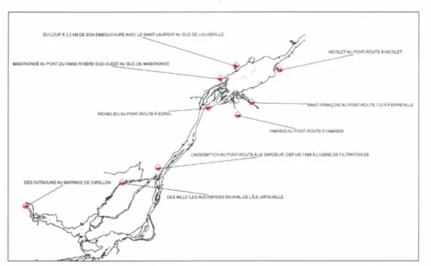
The St. Lawrence River water temperature is strongly influenced by the temperature of the inflowing tributaries. They have a major influence especially on riparian shallow water areas. Water temperature data for several tributaries where collected by the Ministère de

l'Environnement du Québec and extracted from the Banque de données sur la qualité du milieu

aquatique. Figure 1 illustrates the tributary water temperature stations that were used. Water temperature measurements were used to produce simple predictive models linking discharge and accumulated degree-days. We used the available measure of temperature for the early portion of

the year and only the data with a maximum of 600 degree-days.

OU LOUP Â 3,2 KM DE SON EMBOUCHURE AVEC LE SAlNT·LAURENT AU SUD DE LQUISEVlLLE

MASKINONO~ AU PONT OU RANa RM~RE Suo.OUEST AU SUD DE MA$I<lNONOè:

~----""NT.FRANÇOIS AU PONT·ROUTE , 32 ;"PIERREVILLE

RICHELIEU AU PONT.ROUTE;' SOREL

~

YAMASKA AU PONT· ROUTE À VAMASKA

L'ASSOMPTION AU PONT-RouTE ALE GARDEUR; DEPUIS 111119;" LVSINE DE FILTRATION DE

DES MILLE iLES NJX RN'IDES EN AVItL DE L îlE JAROUAILLE

Figure 1: Location of temperature measurement stations associated with main tributaries

2.2 20 Temperature model: structure and use

2.2.1 Hydrology and numerical field model

Prior to this study, significant efforts have been invested into the simplification of the hydrologic characterization (Morin and Bouchard, 2001; Morin et al. 2003) by the use of discharge scenarios. These scenarios where used for bidimensional simulations of the most important physical drive of the system, such as hydrodynamics, wind waves, light penetration and other physical variables of the St. Lawrence River ecosystem. The uses of the hydrological scenarios allow the production of water temperature simulations that covers the entire spectrum of St. Lawrence River spring hydraulicity with a relatively small number of simulations. Detailed methodologies on digital terrain model preparation, hydrodynamic modelling, and calibration an

validation ofhydrodynamic models can be found in Morin et al. 2001 ;2002;2003.

2.2.2 Hydrodynamic model

The hydrodynamic results are fundamental information that is used by the water temperature mode!. Hydrodynamic modelling was performed using the HYDROSIM model developed at INRS-Eau (Leclerc et al. 1995). The approach used is based on the two-dimensional finite element discretisation of the St. Venant equations (flux formulation), which are solved using an iterative transient solution method named Euler-GMRES (Heniche et al. 1999). It solves simultaneously the mass and momentum conservation princip les, and takes into account the local friction coefficient for parameterization. The turbulence closure scheme uses the mixing length

theory (O-equation model) which involves the horizontal velocity gradients. Vertically integrated, the model produces reliable predictions of mean velocity of the water column, water level, and specific discharge for a wide range of hydrological conditions. The model solves the wetted surface since it incorporates a drying-wetting functionality that allows dynamical estimates of the flow boundary.

As one seeks the steady-state conditions, the solution is considered independent of the initial conditions. As for the boundary conditions scheme, one usually solves the problem using a

specified dis charge at the upstream boundary, water level at the main outlet and specified discharges at the tributary and secondary outlets. Moreover, tangent velocities are imposed as

nul!. For a closed lateral boundary, the drying-wetting functionality is equivalent to imposing a

zero normal flux and a slip flow condition.

2.2.3 Water temperature model

In natural, rivers water temperature is mainly controlled by climatologic parameters like: solar radiation, air temperature, atmospheric pressure, relative humidity, precipitation and wind

Chapitre 2, Methodology

2000) are the basic equations of a water temperature model. Water temperature simulation capabilities are added to the equations by implementing the water column heat balance. This addition helps in the identification within the model of all heat sources and sinks. Thus, the total heat flow rate S contributing in the heat balance of the water colurnn can be expressed as :

where Sa, Sb and Si are respectively heat flow rates between the atmosphere, between the river bed and between the ice cover.

Atmospheric heat flow rate Sa is normally the most important in the total heat flow rate S. The atmospheric heat flow is calculated by solar radiation, infrared radiation evaporation, convection and precipitation.

weighted by an extinction!extinc function.

The river bed heat flow rate can be an important factor, especially into shallow water areas. Determination of Sb can be very challenging. To help with the determination of Sb underground temperature was considered as constant and the thermal convection law was used to represent the heat flux rate with the river bed:

where Kb and Tb are respectively the heat flux coefficient and underground temperature.

In northern cold areas, the estimation of the ice cover's heat flux rate is mandatory. The estimation of the heat flux is done with the following relationship, with negligible frazil ice concentration hypothesis:

where Ki is the heat flux coefficient.

2.2.4 Mathematical model

A depth-averaged bidimensional transport-diffusion equation forms the basis of the water temperature model. With the hypothesis of steady state hydrodynamic conditions, the partial differential equation in non-conservative format is:

m

m m

ô

m

m

ô

m

m

H-+H(u-+v-)--H(D - + D - ) - - H ( D - + D - ) +

ôt

a

0;

a

xxa

xY0; 0; YX

a

YY0;

o S QH(T-T ) - - = 0

pep

where t and (x, y) are time and carte sian coordinates; T, is the depth averaged temperature (unknown); H water depth ; u and v are the velo city components ;

Q

heat discharge by volume unit coming from tributaries or underground sources, and Ta its temperature. In the last term, S, p and cp are heat flux rates presented earlier, the density and the water specific heat. Dispersion coefficients Dxx, Dyy, Dxy=Dyx are derived form the hydrodynamic results and are adjusted during the calibration process to represent observed data.

This complex equation system is temporally resolved after imposing boundary conditions and pro vi ding an initial solution to the system. Water temperature at the inflow boundary is considered as a function of time while at the outflow, it is considered free condition to be a

(ôl'/Ôtl = 0). Moreover, in dried zones, water temperature and water depth are imposed at zero.

2.2.4.1 Numerical implementation

The water temperature model uses two types of properties, the global properties and the nodal properties. The global properties are time and space constants (Table 1) while the nodal properties (Table 2) can have different values for each calculated node in the domain. For calculation and optimisation purposes, it was decided to use a maximum of global properties (physical data) whenever possible.

Table 1: Global properties of the temperature model

Diffusivity Water lce Properties Meteorological Field

Properties data data

DM, ~v, ~H, p, cp pi, Cpi, Li Patm Tb

~L

The Table 1 lists the 13 global properties: • Molecular dispersion DM;

• Dispersion weighting coefficient ~v, ~H and ~L;

• Water properties p and cp; • Ice properties pi, Cpi and Li; • Atmospheric pressure P atm; • Underground temperature Tb; • Regression coefficient AI and BI.

Regression coefficients

Chapitre 2, Methodology

Table 2: Nodal properties of the temperature model

Field data Hydrodynamic data Meteorological data

u, v, H, DH , Dv

Table 2 shows the 16 selected nodal properties for field (3), hydrodynamic (5) and meteorological (11). Field data include:

• River bed heat flux rate coefficient Kb; • Vegetation cover (in %) SF ;

• Water turbidity r. Hydrodynamic data include :

• Water velocity component u and v; • Water depth H;

• Dispersion coefficient D H and Dv.

Meteorological data and derived variables include: • Solar radiation Hsi ;

• Air temperature Ta ; • Air emissivity Ca; • Relative humidity RH ;

• Wind function f(Wz);

• Precipitation: rain pr if Ta20 'C or snow ps if Ta < 0 'C ; • Ice cover heat flux rate coefficient Ki;

• Extinction function!extinc.

3. Results

3.1 Synthetic climatic series for the St. Lawrence River; completion of

climatic data at Dorval station

3.1.1 Cloud cover

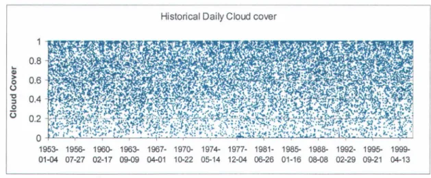
The time-series of cloud cover was recorded at Dorval station for the entire period (1953-2000). No missing data were observed for the daily values. No other post-processing was performed on cloud cover data. Figure 2 presents the daily cloud cover for the entire period (1953-01-01 to 2000-12-31).

...

QI > o U '0 ::J o (3 0.8 0.6 0.4 0.2

Historical Daily Cloud cover

O ~~~~~~~--~~-,~~~~~~~~~~~~~~~~~~

1953- 1956- 1960- 1963- 1967- 1970- 1974- 1977- 1981- 1985- 1988- 1992- 1995-

1999-01-04 07-27 02-17 09-09 04-01 10-22 05-14 12-04 06-26 01-16 08-08 02-29 09-21 04-13

Figure 2: Complete series of the daily cloud cover for Dorval station

3.1.2 Relative humidity

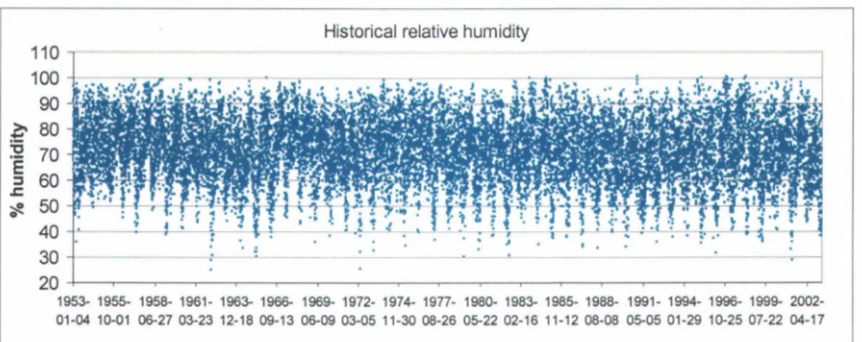
The time-series of relative humidity was recorded at Dorval station for the entire period (1953-2000). No missing data were observed for the daily value. No other post-processing was performed on Relative humidity data. Figure 3 presents the relative humidity for the entire period (1953-01-01 to 2000-12-31).

Historical relative humidity 110 100 90 ~ 80

:a

'Ë :s .c ~ 0 70 60 50 40 30 20 1953- 1955- 1958- 1961- 1963- 1966- 1969- 1972-1974- 1977- 1980- 1983- 1985- 1988- 1991- 1994- 1996- 1999- 2002-01-04 10-01 06-2703-2312-1809-1306-0903-0511-3008-2605-2202-16 11-1208-0805-0501-2910-2507-2204-17

Figure 3: Complete series of the relative humidity for Dorval station

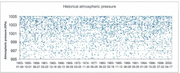
3.1.3 Atmospheric pressure

The time-series of atmospheric pressure was recorded at Dorval station for the entire period of interest. Missing data were observed in the daily values. Missing data replacement was performed using atmospheric pressure data measured at the Saint-Hubert station which is the c10sest station with long time series. The correspondence of atmospheric pressure between the two stations was calculated with observed daily data. Figure 4 illustrates the results of the correspondence analysis.

Atrrospheric pressure correspondance

1050 ~---. 1040 , -1030, -1020 ,- - - : 1010 +-- - - , 1000 -j- - - ; 990 -1-- - ---=-1 R2 = 0.9961 980 +---c~"""-- -970 +---~---~--~--~--~ 960 980 1000 1020 1040 1060

St-hubert station Atmospheric pressure (kPa)

Chapitre 3, Resu/ts

Figure 5 shows the results of the missing data replacement exercise for the atmospheric pressure at Dorval station with Saint-Hubert station data. The missing data replacement procedure produced a complete series of daily values for the entire period (1953-01-01 to 2000-12-31).

1005 ~ 1003 ! ~ 1001 ~ ~ 999 ·C QI .::; ~ 997 E :( 995

Historical atmospheric pressure

1953- 1955- 1958- 1961- 1963- 1966- 1969- 1972- 1974- 1977- 1980- 1983-1985-1988- 1991- 1994- 1996- 1999-

2002-01-04 10-01 06-2703-2312-1809-13 06-0903-05 11-30 08-26 05-2202-16 11-12 08-0805-0501-29 10-25 07-2204-17

Figure 5: Complete series of the daily atmospheric pressure for Dorval station

3.1.4 Air temperature

The time-series of air temperature was recorded at Dorval station for the entire period (1953-2000). No missing data were observed for the daily values. No other post-processing was performed on this series. Figure 6 presents the air temperature for the entire period (1953-01-01 to 2000-12-31).

Historical air temperature

30~~==~====~======~

20

-30+-~-+~--~--~--~~--~--~~~--~~--~--~--r-~~~--~--~

1953- 1955- 1958- 1961- 1963- 1966- 1969- 1972- 1974-1977- 1980- 1983- 1985- 1988- 1991- 1994- 1996- 1999-

2002-01-04 10-01 06-2703-2312-1809-1306-0903-0511-3008-2605-22 02-1611-12 08-0805-0501-29 10-2507-2204-17

Figure 6: Complete series of the daily air temperature for Dorval station

3.1.5 Solar radiation

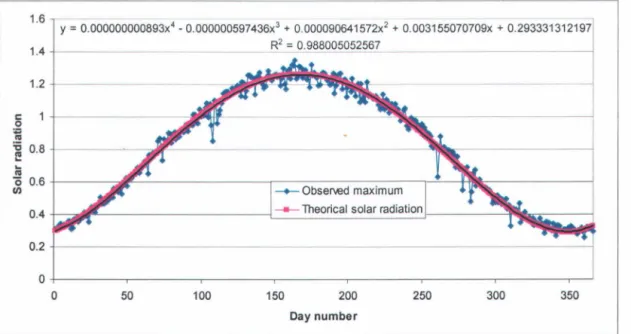
Solar radiation data measured at Dorval station is the series with the most important number of missing data points. The only available data that cou Id be used to fiIl in cover the period between 1988 and 2003 and no other station can provide data for the missing period. Reconstruction of solar radiation was produced by using relationships between theoretical daily solar radiations during the year and observed cloud opacity. Cloud opacity is qualitative data, estimated on a 0 to 10 scale. Both solar radiation and cloud cover are available for the portion 1988 to 2000 of the series. The theoretical function for the maximum solar radiation during the year was built using the interannual maximum measurements of the solar radiation from the available data. A polynomial equation properly reproduces the annual cycle (Figure 7) observed in the solar radiation data.

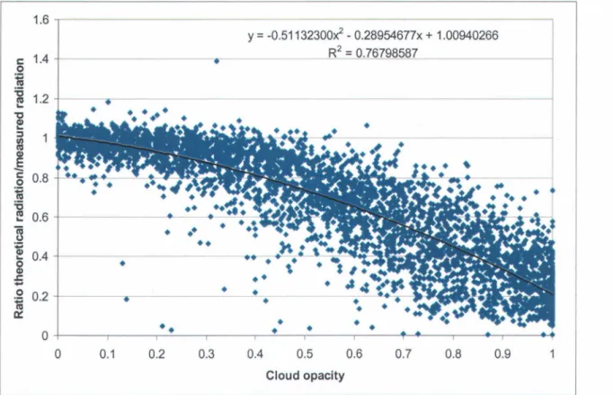
The relation between cloud opacity and solar radiation was built using the ratio of theoretical radiation and measured radiation on measured opacity (Figure 8). The resulting relationship is used to modulate the theoretical solar radiation with the cloud opacity for aIl the time-steps within the considered period. The validation with measured solar radiation gives a satisfactory result. Figure 9 illustrates the high degree of correspondence (r2=0.85) between simulated and measured solar radiation. The completed solar radiation series is shown in Figure 10.

1.6 y = 0.000000000893x4 -0.000000597436x3 + 0.000090641572x2 + 0.003155070709x + 0.293331312197 1.4 _ _ _ _ R 2 _{= 0.988005052567} 1.2 c 1 0 :; ~ _... 0.8 ... CIl Ci 0.6

III -+-Observed maximum

0.4 ----Theorical solar radiation

0.2 0

0 50 100 150 200 250 300 350

Day number

Figure 7: Historical maximum value for measured solar radiations and theoretical model for Dorval station

Chapitre 3, Resu/ts 1.6 , - -y = -0.51132300Jt -0.28954677x + 1.00940266 c 1.4 +---~.---~--~~~==~---~ o

i

:c

_{~ 1.2 +------r---~}

"

~ ~

~

-

c o

i

:c

_cv

_..

0.8 0.6 0.4 0.2 0

•

0 0.1

•

•

•

••

•

••

0.2 0.3

• •

•

-

-.

•

•

•

•

•

0.4 0.5 0.6 0.7 0.8 0.9 Cloud opacity

Figure 8: Relation between observed cloud opacity and the ratio between "theoretical/measured radiations" 1.4 1.2

~

..., ~ c 0 0.8 ~ '6 E ... _{ra 0.6} "0 VI "t:I S _ra 0.4 "5 E ii) _0.2 0 0 0.2 0.4 0.6 0.8 1.2

Measured solar radiation (MJ/m')

Figure 9: Relation between simulated and measured solar radiation for the validation period for Dorval station

Daily solar radiation 1.2 +t-H--t-I-+-H-t-lH-t-+-Hht- +-::-1 .§ ~ ~0.8 ~"~HH"~HI""~~"~~"~~~~~~~~~I~"~~"~~1H c:: o

~ 0.6 . . " . . aJ . . . "~Hf-II1" . . " . . . . I . . . I-.I-.JHI-a1" . . . ~HI-a1IH ... H

:a E li; 004 "0 II) 0.2 -Hr-.-, ... ~H .... I-W-1H . . J,W-I . . . fl...,H . . . . ,....,Hfl . . .

o

+---~~--~--~--~--~~--~--~--~--~~--~---r--~--~~--~ 1953- 1955- 1958- 1961- 1963- 1966- 1969- 1972- 1974- 1977- 1980- 1983- 1985- 1988- 1991- 1994- 1996- 1999- 2002-01-04 10-01 06-27 03-23 12-18 09-13 06-09 03-05 11-30 08-26 05-22 02-16 11-12 08-08 05-05 01-29 10-25 07-22 04-17

Figure 10: Complete series of the daily solar radiation for Dorval station

3.1.6 Precipitation

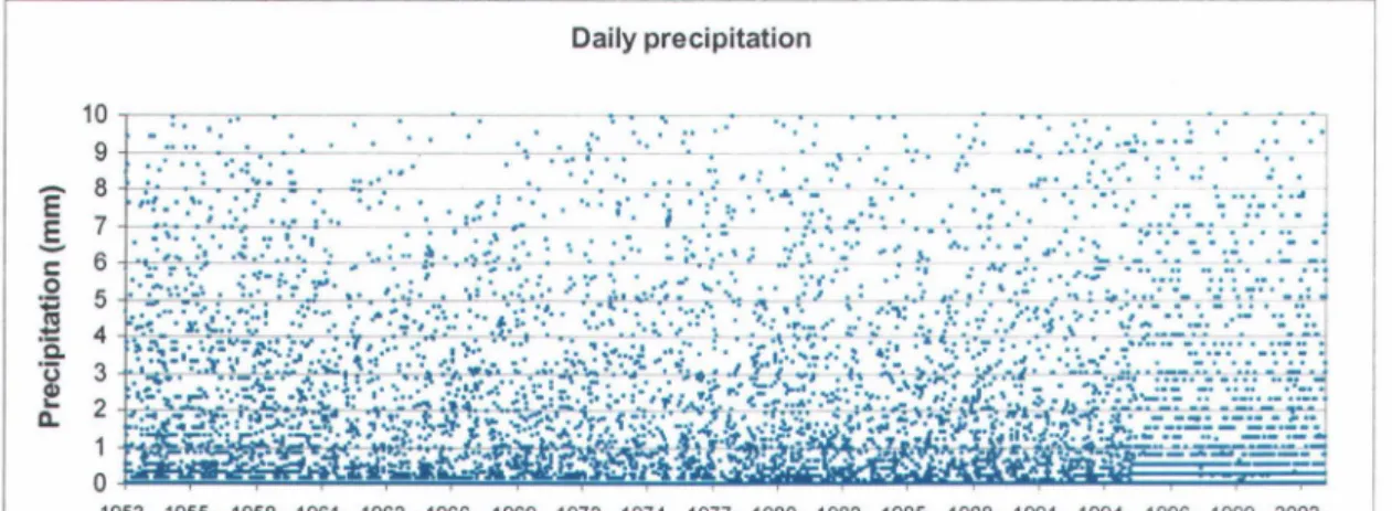
The time-series of precipitation was recorded at Dorval station for the entire period of interest. No missing data were observed for the daily values. No other post-processing was perfonned on these data. Figure Il presents the precipitation for the entire period (1953-01-01 to 2000-12-31).

Ê .§. c:: 0

..

_S 'ë. 'u

e

a.. Daily precipitation 10 9 ~-.. , . • .;" "o • • : " 0. . ': . . 0"0 . ,' • • ~. 0 • • . ; , • • • • • • 0"' • • • • • 1 . . , • 8 7 6 5 4 3 2 1 0

. .. . '-.'

.

'.

~ ~

l

"","",--

-

, .,

,,

.

~ ~~

..

-~f" ""<~ç

u • • •

",;-~

.... "" .. ~.: '.J.;.,~ • .... " .. -:0. o:..:.t ., .. , ... ~". , ... ,."\_o"",.l.I \,,:~.ë.':' ... <1'. _ W.t"·I".I;_.,~:~ • ________ ._._ • - " : ' " -0°":' • • !o., ~ ~ • • , ~.,.~ •• " ' " . . . 0 . " . . . '". ".-"~-:..~~.~ __ ". _ . _ . _

' . • _ . ' "1:",., .. . , . . " , ' . • ._4_ .. = ___ ~_

• ,""" ,'f\:.tI-. r.!. .0". . - . ...

~--1953- 1955- 1958- 1961- 1963- 1966- 1969- 1972- 1974- 1977- 1980- 1983- 1985- 1988- 1991- 1994- 1996- 1999- 2002-01-04 10-01 06-2703-23 12-1809-13 06-0903-05 11-30 08-26 05-22 02-16 11-12 08-0805-0501-29 10-2507-2204-17

Chapitre 3, Results

3.1.7 Wind velocity

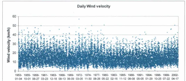
The time-series of wind velocity was recorded at Dorval station for the entire period of interest. No missing data were observed for daily values. No other post-processing was performed on wind velo city data. Figure 12 presents the precipitation data for the entire period (1953-01-01 to 2000-12-31).

Daily Wind velocity 60 50~--- -~

l

40~~~~~~~~~~~~~-~~~~-~---~-~---~~

~ 30

_o

~J~~~~~~~~~~~~~

!

~~~~

~

~

~~

~~F.:~~~~~~~~~

j "C 20 t: ;: 10 O +-~~~~--~~~~~~~--~~--~--~~--~~~~~--~ 1953- 1955- 1958- 1961- 1963- 1966- 1969- 1972- 1974- 1977- 1980- 1983- 1985- 1988- 1991- 1994- 1996- 1999- 2002-01-04 10-01 06-27 03-23 12-18 09-13 06-09 03-05 11-30 08-2605-22 02-16 11-12 08-08 05-05 01-29 10-2507-22 04-17

Figure 12: Complete series of the daily wind intensity for Dorval station

3.2 Temperature boundary conditions for the tributaries and main

inflow

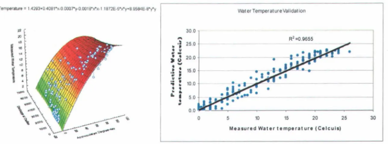
3.2.1 Ottawa River (Carillon Dam)

Figure 13 presents the relationship produced for the Ottawa River at Carillon. The relationship between accumulated degree-days (ADD), discharge and water temperature is highly significant (r2=0.9655). Validation of the relationship was performed with measured water temperature. Figure 13 presents the results of the validation.

Water Temperature = 1.42Q3"'O 4081'x-O OOOT"y-O.OOI a"x"x-l 1872E·S"x"y ... a 9584E-S-y"y _{Water Temperature Validat ion} 30.0 .... • .~ 25.0 R'=0.9655 - - --,..,- --1

• •

: j 20.0 ""

.t :

15.0 M • • M :; ~ 10.0

• •

• • '" ~ 5.0 M 0.0 .,...~~--~--~--~-~---I 10 15 20 25 30 Me3sured Water temperat Uf. 'Calculs)

Figure 13: Relation between degree-days, discharge and water temperature for the Ottawa River and the validation of the resulting model

3.2.2 Des Milles-Iles and des Prairies Rivers

Beeause of the hydrologie al link between the Ottawa River at Carillon and the des Milles-Iles

and des Prairies Rivers, the water temperature of des Milles-Iles and des Prairies Rivers was

direetly eompared to measured water temperature at Carillon to produee a relationship based on

water temperature at Carillon. Figure 14 presents the relationship between Carillon and des

Milles-Iles Ri ver.

Measured wat er t emperat ure Cari Ilon-Milles--Iles

= 30 -M

,

_.... ~ a 25 .~ ] : J 20+--

-,

"" & = 15

-=:

101

-..

.

H

:! :

•

il! y =0.9036x + 1.6651 10 15 20 25

Rivière s de 5 M 11I8s·118 1 wat e r tempe rat ure (Ce le 1 us)

30

Figure 14: Relation between Ottawa River and the Des Milles-Iles River temperature

3.2.3 L'Assomption River

Figure 15 presents the relationship produeed for l'Assomption River. The relationship between

ADD, diseharge and water temperature is highly signifieant (r2=O.88). Validation of the

relationship was performed with measured water temperatures. Figure 15 presents the results of

Chapitre 3, Resu/ts

Water Temperature::. 1 6028+0 4453-x-O 010S-y-O.002Tx"x-O 0002"'X-y+l 4294E-5·'(y

Water temperature validation

02 = () AA~R 30

:

~ 20 ~

·

·

·

10

·

·

·

·

1 J ₀

·

~ 1 -10

M ••• ur.d Rlvl.r • • A •• ompllon ... I.r 'amper,tur. (C.lelu.)

Figure 15: Relation between degree-days, discharge and water temperature for the Assomption River and the validation of the resulting model

3.2.4 Richelieu River

Figure 16 presents the relationship produced for the Richelieu River. The relationship between

ADD, discharge and water temperature is highly significant (r2_{=0.87). Validation of the}

relationship was performed with measured water temperature. Figure 16b presents the results of the validation.

Water Temperature ::. 5.6B71'i'O.3232"x--O.0004·y-O.001~x"x.2.0462E.e-x"y+ 1 7299E·6"V-y

30 ::J I!! QI ₂₅ ~E_ ₂₀ CJ C? III ~ ~.§ ₁₅ '0 EQi 10 QlQI(,.)

'0-:::-

₅ .- QI ' 0 _ I!! III 0 c.. ~

Water temperature validation

---..

_,

.

~!d'~>-I--'-__ __ --bl~.FI1.E:..!..J i l : • 0 5 10 15 20 • •

..

25 30

Measured Richelieu water temperature (Celcius)

Figure 16: Relation between degree-days, discharge and water temperature for the Richelieu River and the validation of the resulting model

3.2.5 Yamaska River

Figure 17 presents the relationship produced for the Yamaska River. The relationship between

ADD, discharge and water temperature is highly significant (r2=O.85). Validation of the

relationship was performed with measured water temperature. Figure 17b presents the results of the validation.

Watertemperature = 2.4455+0.39Il"x-O.005Ty·O.0019"x'x· 1 793BE-5'x'y+B.5933E-Il"y"y , - - - -- - - - ,

Water temperature validation

10 ~ 40 ~ en 10 ::J ₃₀ -E-~ 10 ~ ~ 20 >- Q. 'ü '0 _{E'ai 10} .!CI>O 10 - - 0

-

_::J

...

_CI> E ni -10 .10 20 30 40 in ~

Measured Yamaska water temperature (Celcius)

Figure 17: Relation between degree-days, discharge and water temperature for the Yamaska River and the validation of the resulting model

3.2.6 Saint-François River

Figure 18 presents the relationship produced for the Saint-François River. The relationship between ADD, discharge and water temperature is highly significant (r2=O.87). Validation of the relationship was performed with measured water temperature. Figure 18 presents the results of the validation.

Water temperatl.Jre :: 3 4827+0.3806""x-Q 0043"'y.O.OOl8"x"'x-2 4852E.6'"x"'y+l 9156E.6·Y'Y

30 Water temperature validation

D2 - fi Q')63 30

O ~=q-=---.---r----'---;

-10 20 30

Measured Saint-François water temperature (Celcius)

Figure 18: Relation between degree-days, discharge and water temperature for the Saint-François River and the validation of the resulting model

Chapitre 3, Results

3.2.7 Nicolet River

Figure 19 presents the relationship produced for the Nicolet River. The relationship between ADD, discharge and water temperature is highly significant (r2_{=0.88). Validation of the}

relationship was performed with measured water temperature. Figure 19 presents the results of the validation.

Water Temperature = 2 142B.0,4101·x·O 0272·y-O,QO:rX-x+2 1692E-S·X"y+9.8115E-5*'(y

2~ 22

f

:

i 16 ~ 1-4 ! 12

i

10

i

:

30 .,

.

•

•

-

·

.

_{., 20} .~ ~ ~ li: • a

....

,. 10

·

.

~ .,

. .

!

·

M ()

.

.., 0

·

:

..

.

III ~ -10

Water temperature validation R2

=

n 6289

•

• •

10 20 30

Measured Nlcolet water temperature (Celclus)

Figure 19: Relation between degree-days, discharge and water temperature for the Nicolet River and the validation of the resulting model

3.2.8 DuLoup River

Figure 20 presents the relationship produced for the DuLoup River. The relationship between ADD, discharge and water temperature is highly significant (r2_{=0.94). Validation of the} relationship was performed with measured water temperature. Figure 20 presents the results of the validation.

Water Temperature := 0.7582+0.4342·x-O.0464·y-O.0021'X-x+O 000 '·x"y+O.DOO3"'ty

Water tem perature validation

R2 = n AAg7

Measured DuLoup water temperature (Celcius)

Figure 20: Relation between degree-days, discharge and water temperature for the Du Loup River and the validation of the resulting model

3.2.9 Maskinongé River

Figure 21 presents the relationship produced for the Maskinongé River. The relationship between ADD, discharge and water temperature is highly significant (r2_{=0.94). Validation of the}

relationship was performed with measured water temperature. Figure 21 presents the results of

the validation

Water Temperature = 1.1986+Q.3964·x-O 0306"'y-O 00 1 S"x"'x+g 1714E-S·x"y+O 000l·y"y

...

Q) 't:J 1ii _~ Q) ... ~ Q) :J VI ~.~ ~ '5 : J C Q ) -E o o . Q ) .- C E (,) (/):;;:Q)V I -co :E

Water temperature validation

30 20 10 0 -10 .1 10 2Çl

Measured Maskinongé water temperature

(Celcius)

Figure 21: Relation between degree-days, discharge and water temperature for the Maskinongé River and the validation of the resulting model

3.2.10 St. Lawrence River at Beauharnais Dam

Figure 22 presents the relationship produced for the St. Lawrence River at the Beahamois Dam. The relationship between ADD, discharge and water temperature is highly significant (r2

=0.92). Validation of the relationship was performed with measured water temperature.

3D Scatterplot (BEAUHARNOIS.sta 4",'114C)

"VALEUR"· 1.0414+O.0705~-O.0005"y-5.8216E-5"'X"X-l.5133E-S"X"y+5.4 7 4E-8 '"y"y

'" en .2 25 G> u 20 3~ -:ôe 15 e~ (!) E "C Cl> 10 $C. JlI E :l.!! 5 E ~

.

Vl-

...

~

Water tempe rature validation

If = 0.9194

10 15 20 25

Measured Great Lakes water temperature (Celcius)

Figure 22: Relation between degree-days, discharge and water temperature for the St. Lawrence River at Beauharnois Canal and the validation of the resulting model

Chapitre 3, Resu/ts

3.3 Boundary conditions for each quarter-month for 20 temperature

simulations

3.3.1 Global meteorological modeling conditions (QM aggregation)

In order to feed the water temperature model in global and nodal properties, and to meet the Plan of study temporal step, daily meteorological parameters where reduced to QM mean (from the reconstructed daily series) for each QM (1 to 48) of each year. For the 2D simulations we used the "normal" climate, which is the average interannual QM from the available climatic series. Table 3 presents these QM means (normal climate) for the spring time period used in the water temperature model. The QM are used to coyer the entire fish spawning spring period.

Table 3: Climatic conditions used for driving the 20 temperature model in these conditions were used as spatially constant over the entire system

Precipitation

Quarter Cloud Relative Atmospheric Air Solar (mm/day) Wind Humidity pressure

Month Cover % % kPa) temperature (oC) Radiation (MJ) Velocitv (km/h)

9 0.64 71.26 1010.97 -4.68 0.45 0.06 17.40 10 0.65 70.05 1011.39 -3.56 0.50 0.05 16.26 11 0.60 69.36 1010.71 -1.35 0.58 0.05 16.26 12 0.60 67.97 1011.03 1.30 0.61 0.05 16.51 13 0.67 69.10 1008.37 2.66 0.59 0.07 16.85 14 0.59 63.96 1010.82 4.59 0.68 0.05 16.53 15 0.65 65.64 1009.62 7.52 0.67 0.06 16.15 16 0.63 62.90 1010.26 9.03 0.73 0.05 15.30 17 0.61 61.03 1010.25 10.91 0.78 0.07 15.21 18 0.64 64.05 1009.47 12.83 0.77 0.05 15.15 19 0.61 64.78 1009.78 14.52 0.82 0.05 14.25 20 0.61 65.15 1009.51 15.55 0.84 0.05 13.80 21 0.62 67.52 1008.74 16.63 0.84 0.06 13.60 22 0.60 67.71 1008.48 18.06 0.87 0.05 14.11 23 0.59 68.66 1008.98 19.43 0.89 0.06 13.32 24 0.60 69.40 1008.60 19.97 0.86 0.07 13.77

3.3.2 Tributaries water temperature boundary conditions (QM aggregation)

Water temperatures for the tributaries were calculated with the developed relationships presented earlier. The water temperature is a function of accumulated degree-days (ADD) and tributary discharge. In order to feed the relationships, the ADD was previously calculated with daily air temperature data for the entire reconstructed series. ADD was defined as the number of

Oc

over

SOc. Each daily QM value of each year was aggregated using the QM number. To determine the typical ADD of each quarter-month, the mean value of the ADD was used. The predetermined discharge within the hydrological scenarios (Morin and Bouchard 2001; Morin et al. 2003) were used in the tributaries water temperature relationships.

3.3.2.1 Quarter-monthly water temperature simulations

To pro duce reliable water temperature simulations usable for fish spring spawning, an determined QM (9 to 24) were combined to the hydrological spring scenarios (8 scenarios) that cover the entire spectrum of spring hydraulicity. Thus, the total number of simulations (128) can be used for any meteorological or hydrological conditions by using linear interpolation between simulations representing specifie conditions. To pro duce reliable water temperature simulations usable for fish spring spawning, aH determined QM (9 to 24) were combined to the hydrological spring scenarios (8 scenarios) that cover the entire spectrum of spring hydraulicity. Thus, the total number of simulations (128) can be used for any meteorological or hydrological conditions by using linear interpolation between simulations representing specifie conditions. Table 4 present an the water temperature simulation (tributaries water temperature) by hydrological scenarios (1P to 8P) and by QM during spring time (9 to 24). Table S present the accumulated degree days of the normal c1imate corresponding to the simulated conditions ofthe QM 9 to QM 24.

Table 4: Water temperature boundary conditions used for ail 128 temperature simulations (20)

1 P . Î'~3~ 1 .• ;· •• :i7t%(.:!~J(,~:~'<tt(:'·i; .• ,. ':1\~,?':;! 1l0'?l$M'ep·%~, .. Î Î

;B\

QM Outaouais ChateaugL Beauharnois MIP Assomption Richelieu Yamaska St-Francois Nicolet DuLoup Maskinongé

9 1.16 1.56 0.002.98 1.56 4.99 2.43 3.11 1.84 0.46 1.11 10 1.22 1.63 0.02 3.03 1.63 5.04 2.49 3.17 1.90 0.53 1.18 11 1.33 1.74 0.12 3.11 1.74 5.14 2.59 3.27 2.01 0.64 1.28 12 1.65 2.07 0.42 3.36 2.07 5.42 2.90 3.57 2.33 0.99 1.59 13 2.16 2.61 0.90 3.75 2.61 5.87 3.41 4.06 2.86 1.54 2.10 14 2.87 3.36 1.57 4.31 3.36 6.50 4.11 4.73 3.59 2.31 2.81 15 4.12 4.66 2.74 5.27 4.66 7.60 5.33 5.91 4.85 3.66 4.03 16 5.63 6.25 4.17 6.44 6.25 8.94 6.81 7.34 6.39 5.29 5.52 17 7.34 8.04 5.78 7.77 8.04 10.44 8.49 8.95 8.12 7.13 7.20 18 9.12 9.88 7.45 9.14 9.88 12.00 10.21 10.62 9.91 9.03 8.94 19 10.84 11.67 9.07 10.48 11.67 13.50 11.88 12.23 11.63 10.86 10.61 20 12.36 13.23 10.50 11.66 13.23 14.81 13.34 13.64 13.14 12.46 12.08 21 13.79 14.70 11.84 12.77 14.70 16.04 14.70 14.96 14.54 13.96 13.45 22 15.12 16.05 13.09 13.79 16.05 17.18 15.96 16.18 15.83 15.34 14.71 23 16.35 17.29 14.24 14.75 17.29 18.21 17.11 17.30 17.01 16.60 15.87 24 17.48 18.42 15.30 15.62 18.42 19.16 18.16 18.32 18.08 17.75 16.93

Chapitre 3, Resu/ts

2P "',,' Cc 'cc,' ',,,, CC c,\C ,Ci' ", _{d cc, c} cc!/)tti _{~,c.~ ccc}

QM Outaouais ChateaugL Beauharnais MIP Assomption Richelieu Yamaska St-Francois Nicolet DuLoup Maskinongé

9 0,78 1.53 0.55 2.68 1.53 4.90 2.42 3.08 1.79 0.42 1.09 10 0.84 1.60 0.60 2.73 1.60 4.96 2.48 3.14 1.85 0.49 1.15 11 0.94 1.71 0.70 2.81 1.71 5.05 2.58 3.24 1.96 0.60 1.25 12 125 2.04 1.00 3.05 2.04 5.33 2.90 3.54 2.29 0.95 1.57 13 1.75 2.58 1.48 3.44 2.58 5.78 3.40 4.03 2.81 1.50 2.07 14 2.45 3.33 2.14 3.98 3.33 6.42 4.10 4.70 3.54 2.28 2.78 15 3.66 4.64 3.30 4.92 4.64 7.52 5.33 5.88 4.81 3.62 4.01 16 5.14 6.22 4.71 6.06 6.22 8.85 6.81 7.31 6.34 5.25 5.49 17 6.81 8.01 6.31 7.36 8.01 10.36 8.48 8.92 8.07 7.09 7.17 18 8.54 9.85 7.96 8.70 9.85 11.91 10.21 10.58 9.86 8.99 8.91 19 1022 11.64 9.56 10.00 11.64 13.42 11.87 12.19 11.58 10.82 10.58 20 11.69 13.21 10.98 11.14 13.21 14.73 13.34 13.61 13.09 12.43 12.06 21 13.08 14.67 12.30 12.21 14.67 15.96 14.70 14.93 14.49 13.92 13.42 22 14.36 16.02 13.53 13.20 16.02 17.10 15.95 16.15 15.78 15.30 14.69 23 15.54 17.26 14.67 14.12 17.26 18.14 17.10 17.27 16.97 16.56 15.85 24 16.63 18.40 15.71 14.96 18.40 19.08 18.15 18.29 18.04 17.71 16.91 3P jeCY ;, ,:;';:;: I;F~MJ Cc ,ccc,;, ,,,pc, , cf,\\F ' ''', ' ; ''l'!;'cc cà"" I,_,;;~l

QM Outaouais ChateaugL Beauharnais MIP Assomption Richelieu Yamaska St-Francois Nicolet Du Loup Maskinongé

9 0.47 1.38 0.79 2.44 1.38 425 2.37 3.04 1.68 0.30 0.92 10 0.53 1.44 0.85 2.49 1.44 4.30 2.43 3.10 1.74 0.37 0.98 11 0.63 1.56 0.95 2.56 1.56 4.40 2.54 3.20 1.85 0.49 1.08 12 0.93 1.89 1.24 2.80 1.89 4.68 2.85 3.50 2.17 0.83 1.40 13 1.42 2.43 1.71 3.18 2.43 5.13 3.35 3.99 2.69 1.38 1.90 14 2.10 3.18 2.38 3.71 3.18 5.77 4.06 4.66 3.42 2.16 2.61 15 3.28 4.49 3.53 4.62 4.49 6.88 5.28 5.84 4.69 3.51 3.84 16 4.72 6.07 4.93 5.74 6.07 8.22 6.76 7.26 6.23 5.14 5.33 17 6.35 7.86 6.51 7.00 7.86 9.73 8.43 8.88 7.96 6.98 7.01 18 8.02 9.71 8.15 8.30 9.71 11.30 10.16 10.54 9.75 8.88 8.75 19 9.65 11.50 9.74 9.56 11.50 12.81 11.82 12.15 11.47 10.71 10.43 20 11.08 13.07 11.14 10.66 13.07 14.14 1328 13.57 12.98 12.32 11.90 21 12.41 14.53 12.45 11.69 14.53 15.38 14.64 14.89 14.38 13.82 13.28 22 13.64 15.89 13.67 12.65 15.89 16.52 15.90 16.10 15.67 15.20 14.54 23 14.78 17.13 14.79 13.53 17.13 17.57 17.05 17.23 16.86 16.46 15.71 24 15.81 18.27 15.82 14.33 18.27 18.53 18.10 18.25 17.93 17.61 16.77 25

,},:"",/> """" f,/:,;",i::::,:'

_cc,.'

_{,', "<:}

cr

19Y /

,*'

" :8/: :L'

F"'"",,,

: ,j)iitI~ 1}}7:' ",ZZ ~;::i/A}"::Y9·· 4P " " ,,' )'

QM Outaouais ChateaugL Beauharnois MIP Assomption Richelieu Yamaska St-Francois Nicolet DuLoup MaskinongÉ

9 0.29 1.23 0.80 2.31 1.23 3.76 2.30 2.98 1.54 0.30 0.86 10 0.35 1.30 0.86 2.35 1.30 3.82 2.36 3.04 1.61 0.37 0.92 11 0.45 1.41 0.95 2.43 1.41 3.91 2.46 3.14 1.72 0.49 1.03 12 0.75 1.74 1.24 2.66 1.74 4.20 2.78 3.44 2.04 0.83 1.34 13 1.22 2.28 1.71 3.03 2.28 4.65 3.28 3.93 2.56 1.38 1.85 14 1.89 3.03 2.37 3.54 3.03 5.29 3.98 4.60 3.29 2.16 2.55 15 3.05 4.34 3.51 4.44 4.34 6.41 5.20 5.78 4.56 3.51 3.79 16 4.45 5.93 4.89 5.53 5.93 7.75 6.68 7.20 6.10 5.14 5.28 17 6.04 7.72 6.46 6.76 7.72 9.28 8.35 8.82 7.83 6.98 6.96 18 7.68 9.57 8.08 8.03 9.57 10.85 10.08 10.48 9.62 8.88 8.70 19 9.26 11.36 9.65 9.25 11.36 12.37 11.74 12.09 11.34 10.71 10.38 20 10.65 12.94 11.03 10.33 12.94 13.71 13.20 13.51 12.85 12.32 11.85 21 11.94 14.40 12.32 11.33 14.40 14.96 14.56 14.82 14.26 13.82 13.23 22 13.13 15.76 13.52 12.25 15.76 16.11 15.82 16.04 15.55 15.20 14.50 23 14.22 17.01 14.62 13.10 17.01 17.17 16.96 17.16 16.73 16.46 15.66 24 15.22 18.14 15.64 13.87 18.14 18.14 18.01 18.18 17.81 17.61 16.72 5P ))\';'\1;): _{.. :,: H;t';: J':"i " lu.yF:. 1$::'.::}

1'1

,,;f _{.. ,' ):Z I.,J} 2~~ :~.,

QM Outaouais Chateaugu Beauharnois MIP Assomption Richelieu Yamaska St-Francois Nicolet DuLoup Maskinonge

9 0,21 0,12 0,61 2,24 0,12 3,05 1,92 2,39 0,77 0,00 0,19 10 0,27 0,19 0,67 2,29 0,19 3,11 1,98 2,45 0,84 0,00 0,26 11 0,37 0,30 0,77 2,36 0,30 3,20 2,08 2,55 0,94 0,00 0,36 12 0,66 0,64 1,06 2,59 0,64 3,49 2,39 2,85 1,27 0,12 0,68 13 1,13 1,18 1,52 2,95 1,18 3,96 2,89 3,33 1,79 0,68 1,19 14 1,78 1,94 2,17 3,46 1,94 4,61 3,59 4,01 2,53 1,46 1,90 15 2,92 3,26 3,31 4,35 3,26 5,74 4,81 5,19 3,80 2,81 3,14 16 4,30 4,86 4,68 5,41 4,86 7,11 6,28 6,61 5,34 4,45 4,64 17 5,86 6,68 6,24 6,62 6,68 8,66 7,95 8,22 7,08 6,30 6,34 18 7,47 8,55 7,85 7,86 8,55 10,27 9,66 9,88 8,87 8,21 8,09 19 9,01 10,36 9,40 9,06 10,36 11,82 11,32 11,49 10,60 10,06 9,78 20 10,37 11,95 10,78 10,11 11,95 13,19 12,77 12,90 12,11 11,68 11,27 21 11,63 13,44 12,06 11,09 13,44 14,46 14,13 14,22 13,52 13,19 12,66 22 12,79 14,82 13,24 11,99 14,82 15,65 15,37 15,43 14,82 14,58 13,94 23 13,85 16,09 14,34 12,81 16,09 16,74 16,52 16,55 16,01 15,86 15,11 24 14,81 17,24 15,34 13,56 17,24 17,73 17,55 17,57 17,09 17,02 16,19

Chapitre 3, Resu/ts

6P l'''> ,/J"'~', ;>~t ;,,;; , , ' ';:;/ 0/'''''';;;'6;/

;"~>H>.;:\\ , !t{t~t;(:i(; I;HE; ,ilIj';; "

QM Outaouais ChateaugL Beauharnois MIP AssoJ11)tion Richelieu Yamaska St-Francois Nicolet DuLoup MaskinongÉ

9 0,26 0.00 0.52 2,28 0.00 3.72 1.43 1.77 0.40 0.00 0.00 10 0.31 0.00 0.58 2.32 0.00 3.77 1.49 1.83 0.46 0.00 0.00 11 0.40 0.00 0.68 2.39 0.00 3.87 1.59 1.93 0.57 0.00 0.00 12 0.68 0.00 0.97 2.61 0.00 4.17 1.90 2.23 0.89 0.00 0.00 13 1.13 0.00 1.43 2.95 0.00 4.64 2.40 2.71 1.42 0.27 0.22 14 1.75 0.69 2.08 3.43 0.69 5.30 3.10 3.38 2.15 1.06 0.95 15 2.82 2.04 3.21 4.27 2.04 6.45 4.31 4.56 3.43 2.43 2.20 16 4.12 3.67 4.58 5.28 3.67 7.84 5.78 5.98 4.97 4.09 3.73 17 5.59 5.52 6.14 6.41 5.52 9.42 7.43 7.59 6.72 5.97 5.45 18 7.09 7.43 7.74 7.57 7.43 11.06 9.14 9.25 8.52 7.91 7.24 19 8.53 9.29 9.30 8.69 9.29 12.64 10.79 10.85 10.25 9.79 8.96 20 9.79 10.92 10.66 9.67 10.92 14.04 12.23 12.26 11.77 11.44 10.48 21 10.95 12.45 11.94 10.56 12.45 15.35 13.57 13.57 13.19 12.98 11.89 22 12.01 13.87 13.12 11.39 13.87 16.56 14.81 14.79 14.49 14.40 13.21 23 12.97 15.17 14.22 12.13 15.17 17.68 15.95 15.90 15.69 15.70 14.41 24 13.84 16.37 15.21 12.80 16.37 18.70 16.98 16.92 16.77 16.89 15.52

.•

'xé

' , ' , 7P ;,',' ~',/cc .,,' ,

QM Outaouais Chateaugl Beauharnais MIP Assomption Richelieu Yamaska St-Francois Nicolet DuLoup Maskinongé

9 1.24 0.00 0.41 3.04 0.00 5.44 0.78 1.33 1.26 0.00 0.00 10 1.29 0.00 0.46 3.08 0.00 5.49 0.84 1.39 1.33 0.00 0.00 11 1.37 0.00 0.56 3.14 0.00 5.58 0.94 1.49 1.44 0.00 0.00 12 1.63 0.00 0.85 3.34 0.00 5.83 1.25 1.79 1.76 0.00 0.00 13 2.03 0.00 1.31 3.66 0.00 6.24 1.75 2.27 2.29 0.32 0.11 14 2.60 0.58 1.96 4.09 0.58 6.82 2.44 2.94 3.03 1.11 0.84 15 3.58 1.95 3.09 4.85 1.95 7.82 3.64 4.11 4.31 2.49 2.10 16 4.76 3.61 4.46 5.77 3.61 9.04 5.10 5.53 5.87 4.15 3.63 17 6.08 5.50 601 6.79 5.50 10.43 6.75 7.14 7.62 6.03 5.36 18 7.42 7.45 7.61 7.83 7.45 11.89 8.44 8.79 9.43 7.98 7.15 19 8.70 9.34 9.16 8.82 9.34 13.31 10.08 10.39 11.18 9.86 8.88 20 9.80 11.01 10.52 9.67 11.01 14.57 11.51 11.80 12.72 11.51 10.41 21 10.81 12.57 11.80 10.45 12.57 15.77 12.84 13.11 14.14 13.05 11.83 22 11.71 14.03 12.98 11.15 14.03 16.89 14.07 14.32 15.46 14.47 13.15 23 12.52 15.37 14.06 11.78 15.37 17.95 15.19 15.43 16.66 15.78 14.36 24 13.23 16.60 15.06 12.33 16.60 18.93 16.21 16.44 17.76 16.97 15.47 27

8P _{IZ •.} c y,' t.;;~,

'

".c':cq • 1~2~ilV;

l,'.

:~u:Îs ..

IT

QM Outaouais Chateaugl Beauharnais MIP Assorrption Richelieu Yamaska St-Francois Nlcolet DuLoup Maskinongé

9 3,05 0.00 0.25 2.43 0.00 5.90 0.44 1.23 6.11 0.00 0.00 10 3.09 0.00 0.30 2.47 0.00 5.95 0.50 1.29 6.17 0.00 0.00 11 3.17 0.00 0.40 2.55 0.00 6.04 0.60 1.39 6.28 0.00 0.00 12 3.40 0.00 0.69 2.76 0.00 6.29 0.91 1.68 6.61 0.00 0.00 13 3.77 0.00 1,15 3.11 0.00 6.70 1.41 2.17 7.14 0.47 0.09 14 4.29 0.73 1.80 3.60 0.73 7.27 2.10 2.84 7.89 1.26 0.82 15 5.19 2.11 2.92 4.46 2.11 8.28 3.30 4.01 9.18 2.64 2.08 16 6.26 3.78 4.29 5.50 3.78 9.50 4.75 5.43 10.75 4.31 3.61 17 7.45 5.67 5.83 6.69 5.67 10.89 6.39 7.03 12.52 6.20 5.35 18 8.65 7.63 7.43 7.93 7.63 12.34 8.08 8.68 14.35 8.15 7.14 19 9.78 9.54 8.97 9.15 9.54 13.76 9.71 10.28 16.11 10.03 8.87 20 10.74 11.22 10.33 10.23 11.22 15.03 11.13 11.68 17.66 11.69 10.40 21 11.61 12.79 11.60 11.26 12.79 16.22 12.46 12.99 19.11 13.23 11.82 22 12.38 14.26 12.78 12.23 14.26 17.35 13.68 14.20 20.44 14.66 13.14 23 13.05 15.61 13.86 13.14 15.61 18.40 14.80 15.31 21.66 15.98 14.36 24 13.62 16.85 14.85 13.98 16.85 19.38 15.81 16.32 22.78 17.18 15.47

Table 5: Accumulated degree-days for the "normal" climate, representing the interannual mean of QM, from 1953 ta 2000 (number of degree oC over 5 OC)

Time in QM Accumulated (quarter- degree-days month) oC 9 0.5 10 0,6 11 0.9 12 2.5 13 5.5 14 10.0 15 22.9 16 41.3 17 70.2 18 109.9 19 159.5 20 212.2 21 271.3 22 336.4 23 409.7 24 487.2

Chapitre 3, Resu/ts

3.4 Calibration of diffusivity

in

the 20 temperature model

Lateral and longitudinal diffusion is the main factor controlling the temporal and spatial extent of

a water masse within the river. In the model, it represents the impacts from turbulence and shear

stress occurring in the river. This diffusivity is a nodal property that is derived from the hydrodynamic field; it can be controlled in the model by adjusting the "diffusivity coefficient". Calibration of this coefficient is a mandatory step for aIl transport-diffusion models.

In this study, we used temperature data calculated from remote sensing images for the calibration of the diffusivity coefficient. Remote sensing has the advantage of covering a large area instantaneously and gives a synthetic observation of the general temperature pattern of water

masses. The thermal band (10.4-12.5 um) of Landsat-7 satellite was used to convert numerical

values to surface water temperatures following a methodology from Bartoliucci and Chang

(1988). The Landsat-7 image used for calibration was acquired on May

i

h 2001. Prior to the

calibration of diffusivity, hydrodynamic conditions of May

i

h 2001 were simulated and were

combined with meteorological data of QM 15 in the temperature model. These meteorological

data were used because of their similarity with meteorological conditions of May

i

h 2001. Water

temperature of tributaries (boundary conditions) were determined using the Banque de données

sur la qualité du milieu aquatique of the Ministère de l'Environnement du Québec which had

available data on the same day for most tributaries of the St. Lawrence River. The result is a 2D

simulation of water temperatures that is used to calibrate the diffusion coefficient. The following section presents data produced with the final calibration.

3.4.1 Lake Saint-Louis calibration

The Figure 23 illustrates the results of a water temperature simulation and Landsat-7 image for

the best calibration event. Note that the absolute values of water temperatures cannot be

compared directly, simply because the Landsat-7 image was not calibrated with ground-truth

data. AIso, the Landsat-7 image gives the surface water temperature while the water temperature model gives the depth-averaged temperature. However, general patterns of water temperature

mainly associated with different water masses can be compared. Generally, the model is able to

reproduce the warmer conditions in shallow areas, especially in the Pointe-Claire Bay and at the

south of Île de la Paix. In this area, the model is able to reproduce the cold water coming from

the south of Île de la Paix. AIso, the water temperature delimitation between the Ottawa River

water and the Great Lakes river water is weIl reproduced by the model. There is an important

difference in the general pattern in the north-eastern portion of the lake, which shows a relatively

abrupt decline in water temperature that is not present in the model. We can not explain this situation; it might be associated with the presence ofwater vapour (faint clouds) in the area or an artefact of rapid cooling in the area the night before (not obvious in the hourly temperature data). This image is an instantaneous shot of the lake while the 2D model is considered to represent a steady state. No other images of the spring conditions were found because of the dense cloud

coyer during satellite passages over the area. However, we found an image from fall (November

Il th, 1999) that shows an inverse situation in term of thermal pattern but with a very similar

pattern in term of diffusion. Figure 24 shows a very similar pattern with the inverse thermal

contrast, a typical situation for fall: warmer temperatures in the main water mass and cooler in

shallower areas and in Ottawa River waters. Aiso notice the impact of topographical features like the Iles de la Paix area or the shoals located in the central portion of the lake, north east of Ile Perrot.

LANDSAT IMAGE SIMULATED WATER TEMPERATURE

Figure 23: Calibration image showing the temperature description observed by Landsat.7 (May 7th, 2001) and the simulated conditions for the corresponding date in the Lake Saint-Louis area.

Figure 24: Landsat-7 image of Lake Saint-Louis area (November 11th, 1999), typical of the fall conditions and showing a water temperature pattern similar to simulated conditions.

3.4.2 Lake Saint-Pierre calibration

Figure 25 illustrates the results of a water temperature simulation compared to a Landsat-7 image for the calibration event. Overall, the water temperature model is able to reproduce the warmer temperatures in shallow areas, especially in the Saint-Francois Bay, Maskinongé Bay and on the

Chapitre 3, Results

south shore of Lake Saint-Pierre. Warmer temperatures in shallow areas within Sorel's Islands, like Île de Grace and Grande Île are also weIl reproduced. Spatial variations of water temperature patterns caused by the presence of islands and the impact of the main navigational channel in the center of the lake appear to be relatively weIl captured.

LANDSAT IMAGE / . 1 . j' f. ,

.-Figure 25: Calibration image showing the temperature description observed by Landsat-7 (May

i

h 2001) and the simulated conditions for the corresponding date in the Lake Saint-Pierre area

3.5 Lake Saint-Pierre water temperature during fish spawning periods

A total of 128 simulations of2D water temperature were produced to cover the 16 QM and the 8 scenarios representing aIl possible hydraulic conditions. The following figure presents the results of simulations for the Lake Saint-Pierre area only. These simulations represent discharge events 4P to 6P, which are the most frequent during spring time. The simulated QM that are presented also represent the most frequent QM when fish spawning occurred (15 to 19).

4P discharge event

SP discharge event

6P discharge event

3.0 3.7 4.4 5.1 5.8 6.5 7.2 7.9 8.6 9.3 10.0 10.7 11.4 12.1 12.8 13.5 14.2 14.9 15.6 16.2 17.0

Water temperature in Celcius

Figure 26: Simulated water temperature during the fish spawning period in the Lake Saint-Pierre area

The images of Lake Saint-Pierre water temperature simulations show the temporal evolution (QMI5 to QMI9) of the water temperatures at a given discharge (4 to 6P). The figure can also be interpreted in the perpendicular direction which corresponds to the impact of either reduction or increase of discharge on the water temperatures. It can also be interpreted in the diagonal which allows the analysis of the combined change of discharge and climatic parameters (or time based on the normal climate). It also fairly simple to understand that linear interpolation can be used to create any intermediate condition in term of climatic parameters and discharge, which is also true for all of the 128 simulations that cover the entire St. Lawrence River.