Taylor dispersion of nanoparticles

Taylor Dispersion of Nanoparticles

Sandor Balog*‡†_{, Dominic A. Urban}‡†_{, Ana M. Milosevic}†_{, Federica Crippa}†_{, Barbara}

Rothen-Rutishauser†, Alke Petri-Fink*†#

†_{Adolphe Merkle Institute, University of Fribourg, Chemin des Verdiers 4, 1700 Fribourg,}

Switzerland

#_{Chemistry Department, University of Fribourg, Chemin du Musée 9, 1700 Fribourg,}

Switzerland

‡_{These authors contributed equally.}

*_{Corresponding author: sandor.balog@unifr.ch}

Supporting Information

Contents

1. The initial particle concentrations of the samples ... 2

2. The algorithm of smoothing the raw spectra ... 3

3. The effect of smoothing on the taylograms of NPs ... 9

4. Apparent radius of polydisperse NPs determined by the statistical moments ... 11

1. The initial particle concentrations of the samples

The initial particle concentrations (number per vol.) of the suspension were estimated by using a mean radius, assuming truly spherical particles. This assumption per se is inaccurate and results in values lower than the true values. However, when the polydispersity and shape heterogeneity is moderate (model NPs: SPIONs, Au NPs, SiO2 NPs ), the extent of this

systematic error is small. In the case of industrial particles (ZnO, TiO2, Cu), a good estimate of

concentration is not trivial, which is mostly due to the arbitrary shape. Size polydispersity itself is not critical, for it can be shown that in case of spherical particles, one must calculate by using the third raw moment of the distribution of the radius (Michen, Geers et al. 2015). The table below lists the approximate initial particle concentrations of the suspension. The unit is number ofparticles per mL. BSA: 1.7×1018 SPIONs: 1.7×1013 Au NPs: 1.1×1013 SiO2 NPs: 7.5×1013 ZnO powder: 2.5×1012 TiO2 powder: 9.5×1010 Cu suspension: 3.1×1012

2. The algorithm of smoothing the raw spectra

We performed the following steps prior to analyzing the taylograms: First, we selected the relevant interval of the taylogram, and subtracted a non-zero baseline. This baseline-corrected interval we refer to as A_t. A_t was integrated (that results B_t) and divided into equal subsets of k elements, and the average of each subset was computed (C_t). C_t was interpolated by a polynomial function (D_t). Finally, the time derivative of D_t (E_t) estimates the shape of the signal without noise. To test the efficiency of our algorithm, we simulated taylograms with additive and multiplicative Gaussian noise:

(1-SI) W_t = g_t,A+ g_t,M S_t+ Y,

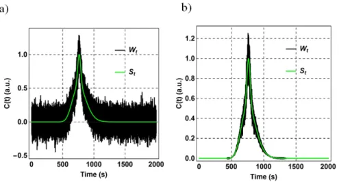
where S_t is the pure signal with an amplitude normalized to one. The additive Gaussian noise (g_t,A) was centered around zero and the multiplicative Gaussian noise (g_t,M ) was centered around one, both with a standard deviation of σ = 0.1. Y represents a randomly chosen constant baseline drawn from a uniform distribution (−0.2 < Y < 0.2). Using Equation 1, we constructed a bimodal signal:

(2-SI) S_t(t, r) = K � y √κ1∙te −(t−t0)2_κ1∙t +_√κ1−y 2∙te −(t−t0)2_κ2∙t �,

where each parameter was drawn randomly from uniform distributions defined respectively by the following closed intervals: 0 ≤ y ≤ 1, 1 s ≤ t₀ ≤ 2000 s, 0.1 s ≤ κ₁ ≤ 10 s, 10 s ≤ κ₂ ≤ 50 s, and K is the amplitude normalization constant. The time resolution was 0.05 s.

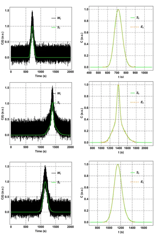
Figure S1 shows the influence of additive and multiplicative noise. While additive noise strongly affects the signal at low values, multiplicative noise is more visible at values closer to the peak center. Figure S2 shows each step of the ‘signal-smoothing’ algorithm, and Figure S3 shows nine results of the smoothing algorithm performed on bimodal signals constructed randomly. In each case, we were able to retrieve the original signal with a high confidence, and the relative differences in the variance V_t and mean M_t (Equation 2 and 3) were on average less

than 5% and 0.5%, respectively. These errors are small, and it is easy to show—by computing the propagation of errors—that the expectable extent of inaccuracy in determining the apparent hydrodynamic radius is confined within the same ranges.

Figure S1. An example of a) additive and b) multiplicative Gaussian noise. The original signal

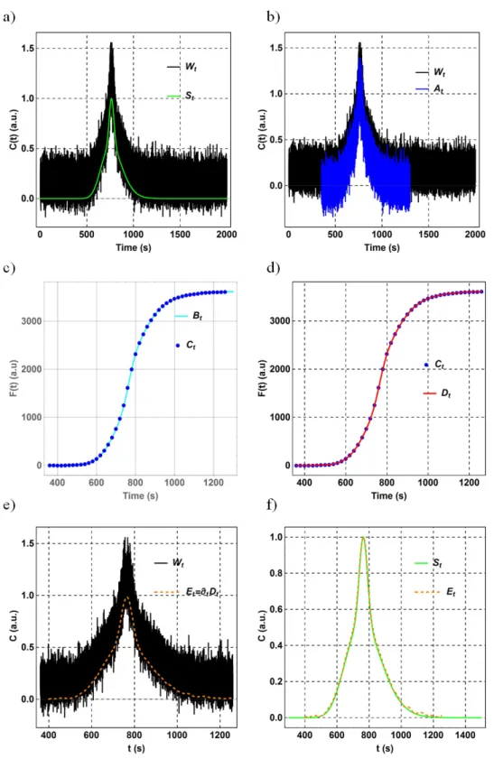
Figure S2. The steps of the smoothing algorithm. a) The signal with noise (black, Equation

1-SI) and the original signal (green, Equation 2-1-SI). b) The baseline-corrected interval selected for further analysis (blue). The baseline was estimated as the average of the first 1000 data points. c) A_t integrated (cyan, B_t) and its moving average (C_t , k = 300). d) Interpolation of C_t

by a polynomial function (D_t). e) The time derivative of D_t (E_t) . f) E_t and the original signal St.

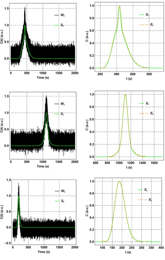
Figure S3-a. Three results of the smoothing algorithm performed on bimodal signals

constructed randomly. Left: the original signals and the signals with noise. Right: the original signals and the signals obtained via the smoothing algorithm.

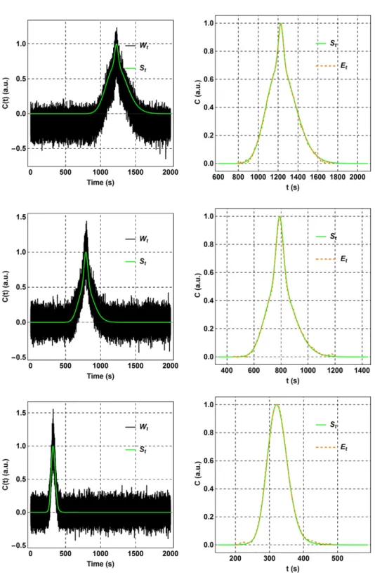
Figure S3-b. Three results of the smoothing algorithm performed on bimodal signals

constructed randomly. Left: the original signals and the signals with noise. Right: the original signals and the signals obtained via the smoothing algorithm.

Figure S3-c. Three results of the smoothing algorithm performed on bimodal signals

constructed randomly. Left: the original signals and the signals with noise. Right: the original signals and the signals obtained via the smoothing algorithm.

Figure S4. The impact of smoothing on the taylograms of the model particles. Left: The

baseline-corrected interval selected for further analysis (blue) and the raw taylogram (black). Right: the smoothed data (orange) and the raw data taylogram (black).

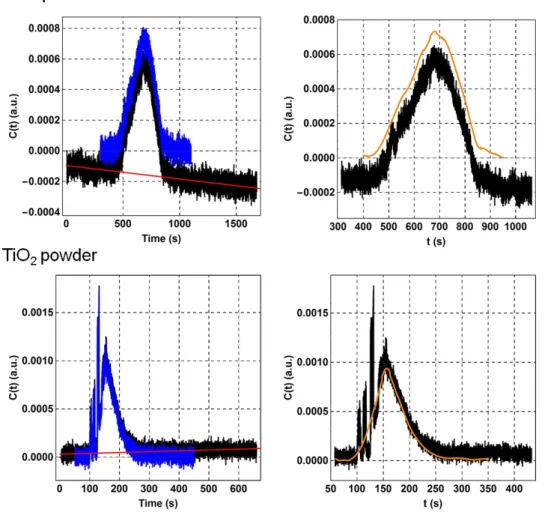
Figure S5. The impact of smoothing on the taylograms of the industrial particles. Left: The

baseline-corrected interval selected for further analysis (blue) and the raw taylogram (black). The baseline was described by a linear function with a non-zero slope. Right: the smoothed data (orange) and the raw taylogram (black). The raw taylograms of the Cu NPs did not need smoothing.

4. Apparent radius of polydisperse NPs determined by the statistical moments

Given that the optical extinction of NPs is a power function of the radius, µ(r, λ) ∝ rn (Quinten 2011 ), the taylogram can be expressed as

(3-SI) C(t) = 1

⟨rn_⟩∙ ∫ P(r) ∙ rn∙ c(t, r) dr

∞ 0

where ⟨rn⟩ is the nth raw moment of the particle size distribution (4-SI) ⟨rn⟩ ≡ ∫ P(r) ∙ r₀∞ ndr.

It is shown below that the mean and the variance of C(t) is

(5-SI) M_t = t₀+δ 2 �rn+1_� ⟨rn_⟩ and (6-SI) V_t ≅ 1 2δ ∙ t0 �rn+1_� ⟨rn_⟩ . The mean (7-SI) M_t ≡ ∫ t ∙ C(t) dt₀∞ (8-SI) M_t = ∫ t ∙ 1 ⟨rn_⟩∙ ∫ P(r) ∙ rn∙ c(t, r) dr ∞ 0 ∞ 0 dt (9-SI) M_t = 1 ⟨rn_⟩∙ ∫ P(r) ∙ rn∙ ∫ t ∙ c(t, r) dt ∞ 0 dr ∞ 0 (10-SI) M_t = 1 ⟨rn_⟩∙ ∫ P(r) ∙ rn∙ �∫ t ∙ c(t, r) dt ∞ 0 � dr ∞ 0 (11-SI) ∫ t ∙ c(t, r) dt₀∞ = t₀+δ∙r 2 (12-SI) M_t = 1 ⟨rn_⟩∙ ∫ P(r) ∙ rn∙ �t0+ δ∙r 2� dr ∞ 0 (13-SI) M_t = 1 ⟨rn_⟩∙ ∫ P(r) ∙ rn∙ (t0) dr + 1 ⟨rn_⟩∙ ∫ P(r) ∙ rn∙ � δ∙r 2� dr ∞ 0 ∞ 0 (14-SI) M_t = t₀ 1 ⟨rn_⟩∙ ∫ P(r) ∙ rn∙ dr + δ 2 1 ⟨rn_⟩∙ ∫ P(r) ∙ rn∙ (r) dr ∞ 0 ∞ 0 (15-SI) M_t = t₀+δ 2 �rn+1_� ⟨rn_⟩ .

The variance (16-SI) V_t ≡ ∫ (t − M₀∞ _t)2∙ C(t) dt. (17-SI) V_t = ∫ (t − M_t)2∙ 1 ⟨rn_⟩∙ ∫ P(r) ∙ rn∙ c(t, r) dr ∞ 0 dt ∞ 0 . (18-SI) V_t = 1 ⟨rn_⟩∙ ∫ P(r) ∙ rn∙ ∫ (t − Mt)2 ∙ c(t, r) dt dr ∞ 0 ∞ 0 (19-SI) V_t = 1 ⟨rn_⟩∙ ∫ P(r) ∙ rn∙ ∫ �t − �t0+ δ 2 �rn+1_� ⟨rn_⟩ � � 2 ∙ c(t, r) dt dr ∞ 0 ∞ 0 (20-SI) V_t = 1 ⟨rn_⟩∙ ∫ P(r) ∙ rn∙ �∫ t2 ∙ c(t, r) dt − �t0+ δ 2 �rn+1_� ⟨rn_⟩ � 2 ∞ 0 � dr ∞ 0 (21-SI) V_t = 1 ⟨rn_⟩∙ ∫ P(r) ∙ rn∙ �∫ t2 ∙ c(t, r) dt − �t0+ δ 2 �rn+1� ⟨rn_⟩ � 2 ∞ 0 � dr ∞ 0 (22-SI) V_t = 1 ⟨rn_⟩∙ ∫ P(r) ∙ rn∙ �t02+ 3 2δ ∙ r ∙ t0+ 3 4δ2∙ r2− �t0 + δ 2 �rn+1_� ⟨rn_⟩ � 2 � dr ∞ 0 (23-SI) V_t = 1 ⟨rn_⟩∙ ∫ P(r) ∙ rn∙ (t02) dr ∞ 0 +_⟨r1n_⟩∙ ∫ P(r) ∙ rn∙ � 3 2δ ∙ r ∙ t0� dr ∞ 0 +_⟨r1n_⟩∙ ∫ P(r) ∙ rn∙ � 3 4δ2∙ r2� dr ∞ 0 +_⟨r1_n⟩∙ ∫ P(r) ∙ rn_{∙ �− �t} 0+δ₂�r n+1_� ⟨rn_⟩ � 2 � dr ∞ 0 (24-SI) V_t = t₀2 +3₂δ ∙ t0�r n+1_� ⟨rn_⟩ +3₄δ2 �rn+2� ⟨rn_⟩ − �t0+δ₂�r n+1_� ⟨rn_⟩ � 2 (25-SI) V_t = t₀2+3 2δ ∙ t0 �rn+1� ⟨rn_⟩ + 3 4δ2 �r n+2_� ⟨rn_⟩ − �t0+ δ 2 �rn+1� ⟨rn_⟩ � 2 (26-SI) V_t = t₀2+3 2δ ∙ t0 �rn+1� ⟨rn_⟩ + 3 4δ2 �r n+2_� ⟨rn_⟩ − t02− t0δ �rn+1� ⟨rn_⟩ − δ2 4 � �rn+1� ⟨rn_⟩ � 2

(27-SI) V_t = 1 2δ ∙ t0 �rn+1_� ⟨rn_⟩ + 3 4δ2 �r n+2_� ⟨rn_⟩ − 1 4δ2� �rn+1_� ⟨rn_⟩ � 2

The right side of Equation 27-SI is dominated by the first term, and finally we obtain that

(28-SI) V_t ≅ 1

2δ ∙ t0 �rn+1�

5. Optical extinction of spherical nanoparticles via Mie calculations

Modelling Au NPs, SiO2 NPs, and SPIONs, we performed Mie calculations to demonstrate

whether the optical extinction is dominated by absorption or scattering. The figures below show the results.

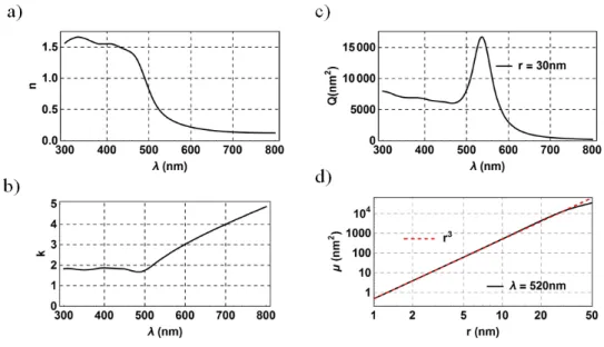
Figure S6. Optical extinction of spherical Au NPs computed via Mie’s theory. a) and b) The

real (n) and the imaginary (k) part of the refractive index used in the calculations. c) The optical extinction as a function of the wavelength of an Au NPs with radius of 30 nm. d) The extinction as a function of the NP radius at the wavelength of 520 nm on a log-log scale. The extinction is proportional to r3 (absorption) on a wide range (red dashed line).

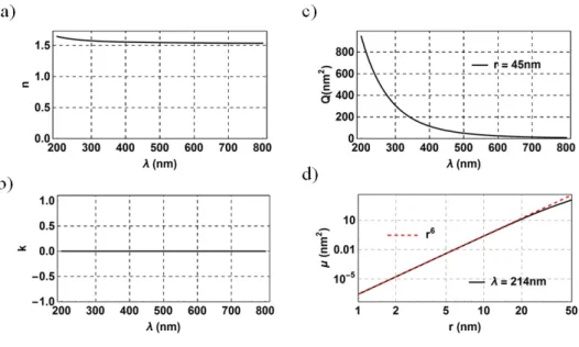
Figure S7. Optical extinction of spherical SiO2 NPs computed via Mie’s theory. a) and b) The

real (n) and the imaginary (k) part of the refractive index used in the calculations. c) The optical extinction as a function of the wavelength of a SiO2 NPs with a radius of 45 nm. d) The

extinction as a function of the NP radius at the wavelength of 214 nm on a log-log scale. The extinction is proportional to r6 (scattering) on a wide range (red dashed line).

Figure S8. Optical extinction of spherical SPIONs (maghemite) computed via Mie’s theory. a)

and b) The real (n) and the imaginary (k) part of the refractive index used in the calculations. c) The optical extinction as a function of the wavelength of a SiO2 NPs with a radius of 8 nm.

d) The extinction as a function of the NP radius at the wavelength of 520 nm on a log-log scale. The extinction is proportional to r3 (absorption) on a wide range (red dashed line).

References

Michen, B., et al. (2015). Avoiding drying-artifacts in transmission electron microscopy: Characterizing the size and colloidal state of nanoparticles. Sci Rep 5: 9793.

Quinten, M. (2011 ). Optical properties of nanoparticle systems: Mie and beyond, Wiley-VCH Verlag GmbH.