Publisher’s version / Version de l'éditeur:
Proceedings of the 23rd International Conference on Port and Ocean Engineering under Arctic Conditions, June 14-18, 2015, Trondheim, Norway, 2015-06
READ THESE TERMS AND CONDITIONS CAREFULLY BEFORE USING THIS WEBSITE. https://nrc-publications.canada.ca/eng/copyright
Vous avez des questions? Nous pouvons vous aider. Pour communiquer directement avec un auteur, consultez la
première page de la revue dans laquelle son article a été publié afin de trouver ses coordonnées. Si vous n’arrivez pas à les repérer, communiquez avec nous à PublicationsArchive-ArchivesPublications@nrc-cnrc.gc.ca.
Questions? Contact the NRC Publications Archive team at
PublicationsArchive-ArchivesPublications@nrc-cnrc.gc.ca. If you wish to email the authors directly, please see the first page of the publication for their contact information.
NRC Publications Archive
Archives des publications du CNRC
This publication could be one of several versions: author’s original, accepted manuscript or the publisher’s version. / La version de cette publication peut être l’une des suivantes : la version prépublication de l’auteur, la version acceptée du manuscrit ou la version de l’éditeur.
Access and use of this website and the material on it are subject to the Terms and Conditions set forth at
Measurements of spatial and temporal variations in ice impact
pressures
Sopper, Regina; Gagnon, Robert; Daley, Claude; Colbourne, Bruce
https://publications-cnrc.canada.ca/fra/droits
L’accès à ce site Web et l’utilisation de son contenu sont assujettis aux conditions présentées dans le site LISEZ CES CONDITIONS ATTENTIVEMENT AVANT D’UTILISER CE SITE WEB.
NRC Publications Record / Notice d'Archives des publications de CNRC: https://nrc-publications.canada.ca/eng/view/object/?id=40c4b939-d54a-4ab6-8452-4c5575c797cb https://publications-cnrc.canada.ca/fra/voir/objet/?id=40c4b939-d54a-4ab6-8452-4c5575c797cb
MEASUREMENTS OF SPATIAL AND TEMPORAL
VARIATIONS IN ICE IMPACT PRESSURES
Regina Sopper1, Robert Gagnon2, Claude Daley1, Bruce Colbourne1
1
Dept. of Engineering and Applied Sciences,Memorial University of Newfoundland, St. John’s, Newfoundland, Canada
2
Ocean, Coastal and River Engineering, National Research Council of Canada, St. John’s, Newfoundland, Canada
ABSTRACT
This paper presents results of laboratory experiments involving a 1 m diameter ice cone colliding with an instrumented panel (Impact Module). The tests were performed using a double pendulum apparatus that provided high impact energy. Images taken with a high speed camera at 500 fps from within the Impact Module provide information about the true contact area and pressure distribution during the collision. The acquired images were translated into pressure distributions using a specifically developed software routine. These data are compared to the output of a separate pressure sensor located in the centre of the Impact Module. The images show increasing contact area as the collision proceeds and capture sudden losses of area as ice fracture and spalling occurred. Observations such as significant spalling events in the vicinity of the central pressure sensor are also reflected in its recordings. The results provide maps of the temporal and spatial variations in contact pressure, contact area and force as an ice impact progresses at speeds typical of impacts that might occur with icebreaking ships.
INTRODUCTION
In 2009 a first series of preliminary impact drop tests were performed on the Impact Module. The tests involved freshwater ice blocks of different masses (up to 130 kg) that were dropped from different heights. A detailed description of the tests and some first results are given in Gagnon et al. (2009). In another study ice crushing tests were performed that were quasi-static in nature and were achieved by pushing a 1 m diameter ice cone into the Impact Module. Some preliminary results of these tests were published in Gudimetla et al. (2012). In both studies the quick response time of the Impact Module to spalling events by showing real-time contact areas during the crushing event has been proven; a feature that makes it preferable to various alternative technologies with longer reaction times, especially considering the extremely fast fracture and spalling events during ice breaking. Here we are reporting on the continuation of tests in more realistic conditions. Large dynamic impact tests have been performed using a unique double pendulum apparatus. The tests were performed in the Structure’s lab at Memorial University of Newfoundland, St. John's, Canada.
POAC’15
Trondheim, Norway
Proceedings of the 23rd International Conference on
Port and Ocean Engineering under Arctic Conditions June 14-18, 2015 Trondheim, Norway
Experimental Setup
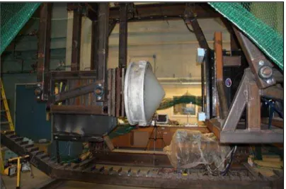
The experimental setup involved a large double pendulum apparatus. A detailed description is given in Gagnon et al. (2015). The apparatus consists of a steel frame of approximately 4 m height with two swinging carriages. The mass of both carriages can be varied and the carriages pulled back to different angles. When the carriages are allowed to swing into each other, impacts with different energy levels at the midpoint can be created. The results
presented in this paper were obtained for a release angle of 35° from the vertical for the swing arms of the pendulums. One carriage supported a 1 m diameter conical ice sample and the other supported the Impact Module as shown in Figure 1.
Ice Specimen
The specimen was made of laboratory grown ice following the procedure given in Gudimetla et al. (2012). Readily available commercial ice was crushed into ice chips with sizes up to roughly 12 mm. The ice seeds were poured into an ice holder set-up and mixed with tap water at a ratio of 2:1. After three to four days of uni-directional freezing in a cold room at -10°C, the blank specimen was shaped into a cone using a purpose- designed shaping apparatus.
Impact Module
The Impact Module is described in detail in Gagnon (2008). It consists of a 1 m x 1 m x 0.46 m acrylic block resting on four flat-jack load-cells to measure impact loads. On the surface of the acrylic block are 13 mm wide, 4 mm thick and approximately 1 m long acrylic strips. The strips are slightly curved in section so when pressure is applied, the strips flatten against the acrylic block. A high speed camera is mounted behind the acrylic block recording at a rate of 500 fps in the present test. The images obtained during a test sequentially show the degree of flattening seen in the acrylic strips and this is used to determine the pressure
distribution.
The module also has 9 strain-gauged acrylic cylinders embedded in the acrylic block to provide direct pressure measurements, one of them right in the centre and only that one will
Figure 1: Large pendulum apparatus with ice cone mounted on the left carriage and Impact Module on the right.
be part of the following analysis. The gauges act as pressure transducers in that if they are subjected to load the cylinders get compressed and the compression is measured by the gauge. This output is given in voltage and converted into pressure by a factor of 14.7 MPa/Volt. The sampling frequency of the pressure plugs as well as of the load cells was 5 kHz.
Image Analysis
Several steps using different software packages were involved in the analysis of the contact area images. The high speed camera behind the acrylic block was mounted on a small block that rested on four silicone pads to compensate for vibration during the dynamic impact. However, the setup allowed some movement in the horizontal as well as vertical directions with respect to the impacted surface. Furthermore the high speed camera was instrumented with a fisheye lens to capture almost the entire area of the pressure panel. These
circumstances resulted in a series of pictures with slightly shifting centres and distortions. This was taken into account by manually processing the images using the software
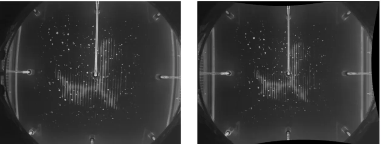
PTLens 8.7.8TM. Each frame was centred, rotated and the lens distortion removed. Figure 2 shows image 18 from the test. In the raw picture on the left the clockwise rotation and the lens distortion are clearly visible. Both these aspects are removed in the corrected image on the right.
The objective of the analysis of the images is to determine the areas where the acrylic strips (white vertical strips in the image) have been compressed and the degree to which they have been compressed. The small white dots that are apparent in both images are air bubbles enclosed in the acrylic block resulting from the casting process.
Figure 2: (Left) Raw image 18 from the high speed camera inside the Impact Module showing the contact area associated with the ice impact that appears as flattening of the pressure strips that covered the surface of the Impact Module. (Right) Image 18 corrected for distortions related to the fisheye camera lens and movement of the camera during the test. Note, the images show a cloud of small air bubbles that are remnants of the acrylic block casting process. These bubbles do not influence results from the experiments.
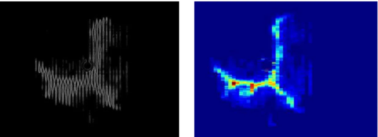
In order to analyse the images the pressure information (i.e. the white vertical strips) needs to be separated from the background of the images. Therefore, a null image for each image was created using Paint Shop Pro 6TM. To do this, first light areas representing the signal from the acrylic strips were shaded to the colour of the background in their vicinity so that the image only showed the background as it is displayed on the left in Figure 3. This null image was
then subtracted from the initial (corrected) image. The resulting image displayed only the acrylic strip contact area. There were some small black holes in the strip areas where air bubbles were located. In order to make up for this area lost due to the subtraction process the black holes were manually filled in to obtain an image, as shown on the right in Figure 3, that is ready for the next stage of analysis.
Figure 3: (Left) Null image of image 18. (Right) Image showing the result of subtracting the null image from the corrected image where only the pressure strip information is visible. In order to convert the pressure strip information of the image to pressure data it is necessary to measure the contact width along each of the pressure strips. To do this efficiently, the pressure strip image was edge-detected using the software ScanProTM. Then a dedicated computer code, written in the software PythonTM was applied to the edge-detected image to determine the width of each strip at all points along its full length. The program converts the width of the strip at each point along its length to the pressure at that point. The result of the edge detection step is shown on the left and the resulting pressure distribution on the right of Figure 4. In addition the software calculates total load, total area, average pressure and maximum pressure.
Figure 4: Close ups of image 18. (Left) Image showing edge detection. (Right) The resulting pressure distribution. A scale of suitable size for viewing is included with the full set of analysed images in the appendix. The width of each image corresponds to 0.64 m.
Test Results and Discussion
The presented results were derived from a test that was performed in the Structures lab of Memorial University of Newfoundland on October 16th, 2014. The release angle of the pendulum arms was 35° from the vertical. The high speed camera recorded at a rate of 500 fps. Of the images that showed the impact, 19 were analysed that covered the ice
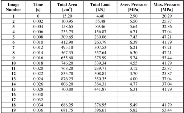
penetration duration of ~ 0.04 s. The first picture exhibiting contact was set to equal time step t = 0. Out of the 19 images, only 17 are presented here. The missing two images 16 and 17 were taken near the end of the ice penetration and were too blurry due to camera motions to yield good results. The 17 images are shown in the appendix. Each contains the respective information for total load, total contact area, average pressure and maximum pressure that is listed in Table 1.
Table 1: Total load, total area, average pressure and maximum pressure received from image analysis. Image Number Time [s] Total Area [cm2] Total Load [kN] Aver. Pressure [MPa] Max. Pressure [MPa] 1 0 15.20 4.40 2.90 20.29 2 0.002 100.95 55.48 5.50 25.87 3 0.004 158.65 89.46 5.64 32.86 4 0.006 233.75 156.87 6.71 37.04 5 0.008 309.65 230.06 7.43 47.21 6 0.010 412.90 263.79 6.39 41.79 7 0.012 495.10 307.53 6.21 47.21 8 0.014 567.35 357.64 6.30 47.21 9 0.016 655.60 375.99 5.74 53.44 10 0.018 746.20 339.34 4.55 41.79 11 0.020 768.20 239.71 3.12 25.87 12 0.022 833.70 308.81 3.70 25.87 13 0.024 876.25 350.35 4.00 37.04 14 0.026 806.20 384.31 4.77 37.04 15 0.028 700.80 441.87 6.31 41.79 16 0.030 - - - - 17 0.032 - - - - 18 0.034 686.25 376.95 5.49 41.79 19 0.036 681.75 396.61 5.82 53.44
For a more comprehensive picture we also looked at the outputs of the centre pressure plug and the load cells behind the acrylic block. In view of the following discussion it is mentioned that the centrally located pressure plug conceals part of the acrylic strips. Hence this small area in the middle of the Impact Module does not contribute information in terms of the image analysis and an offset in the data is to be expected. Therefore, in the data evaluation it must be understood that the information gathered from the image analysis for contact in the central region of the panel will to some extent be underestimating the full contribution from the ice contact. On the other hand, when the action shifts away from the centre, and for larger contact areas, the masking effect of the centre pressure plug is less. Another effect that we note for the reader’s benefit is that the pressures determined from the image analysis are going to be higher than the actual values because the pressure sensing technology was calibrated at 0°C whereas the experiment was conducted at room temperature. 0°C was chosen as the
calibration temperature because the pressure sensing technology is intended for a large impact panel that will be installed on a ship hull for bergy bit impacts in cold water.
The high speed camera and the data acquisition system were not directly synchronized. To synchronize the image data with the rest of the acquired data a few key events, namely the onset of ice contact and some distinct spalling events were identified and matched in the image data and the pressure plug data.
The series of images (appendix) clearly shows a characteristic pressure pattern. Zones of high pressure are surrounded by zones of lower pressures. The former would consist of relatively intact ice whereas the latter would be pulverized spall debris. As the event proceeds, the increasing contact area progressively shows a distinct branching pattern. This was found to be characteristic of all other crushing and impact tests that we conducted using cone shaped ice samples at high rates.
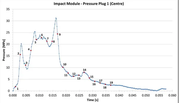
In image 2 the shaded area is rather circular implying that the tip of the ice cone hit the Impact Module in the centre where the pressure plug is located. Subsequent images display high pressure zones emerging in the middle of the contact area as it is indicated in red colours. Up to image 8 these evidently form one fairly large connected area. Between images 9 and 10 a significant spalling event occurred in the vicinity of the pressure plug and was therefore quiet evident in the record in Figure 5. This is shown by the sharp drop in pressure that arose when the portion of the ice contact area that encompassed the pressure sensor suddenly broke away.
Figure 5: Pressure-time history of the centre pressure plug. The red markers and associated numbers correspond to the points in the record when images were acquired.
While it is instructive to study the images individually it is also very useful to view the images in a movie sequence. Dynamic behaviour becomes more evident when the sequence is viewed multiple times. For example the flow of crushed ice (low pressure areas) away from high pressure zones is quite visible from images 9 to 19.
In principal when the pressure patterns are integrated over the whole contact area one should obtain a reasonable value for the total load at that instant in time. However in the present case
we would expect that the integrated values tend to be higher than the actual values of the load cells output. This is due to the temperature at which the pressure strips were calibrated as discussed above. The other factor that comes into play when integrating the pressure is the offset introduced into the data due to the fact that the central pressure plug obscures part of the pressure pattern for centrally located ice contact. We see evidence of both of these effects when we plot the output of the load cells and the load as determined using the image
integration in one graph (Figure 6).
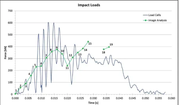
In Figure 6 the load cell record shows large oscillations near the beginning which correspond to resonant oscillations of the Impact Module load sensing system. While these oscillations do not reflect the actual loads, the average values of the oscillations are reasonable estimates of the true load. The data plot of the integrated image loads does not display the oscillations that are apparent in the load cell data because the pressure sensing technology has a significantly higher resonant frequency that is not excited during these tests. Furthermore up to image 10 the load data from the images roughly passes through the average of the oscillations in the load cell data.
Starting with the earlier part of the test (images 1 to 10) we may have expected that all of the load data from the images would have been higher than the values from the load cells as is evident in images 13 to 19. However, the other competing factor (i.e. that part of the area is concealed by the pressure plug) seems to compensate for the overestimation. For images 1 to 10 the pressure plug is centrally located in the pressure patterns and therefore reduces the visible contact areas and the integrated loads. The two competing effects seem to roughly balance out for images 1 to 10. On the other hand in images 13 to 19 the pressure plug is not encompassed by the contact area so it does not influence the integrated image loads.
Therefore for these images only the offset associated with the calibration temperature is present.
Figure 6: Force-time plot of the output of the load cells and the integrated loads of the image analysis.
On the left in Figure 7 the pressure pattern for the last image of the test is shown that occurred when the ice penetration had come to a complete stop. On the right is a photograph of the ice sample after it had been removed from the apparatus. The hard zone area of the impact region is clearly visible as the branching dark area on the contact surface of the ice that corresponds to relatively intact ice. The shape of this hard zone is closely reflected in the pressure
distribution on the left of Figure 7.
Figure 7: (Left) The pressure distribution from a image captured near the end of the impact, i.e. when ice penetration had stopped. The size and shape of the contact region is distinctly different than earlier in the test as shown in the appendix. (Right) A photograph of the impacted ice sample shortly after the ice holder has been removed from the apparatus. The shape of the high pressure contact region, as depicted on the left image, is clearly visible as the darker area of the contact zone. (Taken from Gagnon et al. (2015))
CONCLUSIONS
Overall the Impact Module has been proven to be a useful device to capture pressures and areas during a dynamic ice impact. The true contact areas between ice specimen and Impact Module were well reflected in the images. The analysis showed the development of high and low pressures over the course of the ice impact event.
The total loads and pressures obtained from the image analysis were qualitatively similar to the outputs of the load cells and the central pressure plug. Deviations are considered to be the result of two competing factors; one, being the calibration temperature for the pressure strips and the other being the masking effect of the pressure plug in the image analysis.
Other observation when viewing the images as a movie it is possible to see dynamic aspects such as the flow of crushed ice during the impact test.
It is anticipated that the pressure sensing technology incorporated in the Impact Module will be used in a large impact panel installed on a ship hull for a future field study involving bergy bit impacts.
ACKNOWLEDGEMENTS
The authors would like to acknowledge the financial support of Atlantic Canada Opportunities Agency, Research and Development Corporation, American Bureau of Shipping, BMT Fleet Technology, Husky Energy, Rolls-Royce Marine, Samsung Heavy Industries. Also, we are grateful for the invaluable participation of the National Research Council Canada in the form of providing expertise for all aspects of the apparatus development and experiments, and for the use of a unique scientific instrument. REFERENCES
Gagnon, R.E., 2008. A new impact panel to study bergy bit / ship collisions. Proceedings of 19th IAHR International Symposium on Ice 2008, Vancouver, British Columbia, Canada, Vol. 2, 783-790.
Gagnon, R.E., Bugden, A., Ritch, R., 2009. Preliminary testing of a new ice impact panel. Proceedings of POAC 2009, Luleå, Sweden.
Gagnon, R.E ., Daley, C., Colbourne, B., 2015. A large double-pendulum device to study ice load, pressure distribution and structure damage during ice impact tests in the lab.
Proceedings of POAC 2015, Trondheim, Norway.
Gudimetla, P.S.R., Colbourne, B., Daley, C., Bruneau, S.E., Gagnon, R., 2012. Strength and pressure profiles from conical ice crushing experiments. Proceedings of the international conference and exhibition on performance of ships and structures in ice (ICETECH), Banff, Alberta, Canada.
APPENDIX: 17 Analysed images showing the pressure distribution 1) t = 0 s 2) t = 0.002 s 3) t = 0.004 s 4) t = 0.006 s 5) t = 0.008 s 6) t = 0.010 s 7) t = 0.012 s 8) t = 0.014 s 40 36 32 28 24 20 16 12 8 4 0 40 36 32 28 24 20 16 12 8 4 0
Missing Images at Times 16) t = 0.030 s and 17) t = 0.032 s 9) t = 0.016 s 10) t = 0.018 s 13) t = 0.024 s 14) t = 0.026 s 15) t = 0.028 s 11) t = 0.020 s 12) t = 0.022 s 40 36 32 28 24 20 16 12 8 4 0 40 36 32 28 24 20 16 12 8 4 0
The width of each image in the appendix above corresponds to 0.64 m. The unit on the colour scale is MPa. 19) t = 0.036 s 18) t = 0.034 s 40 36 32 28 24 20 16 12 8 4 0