https://doi.org/10.4224/23000158
READ THESE TERMS AND CONDITIONS CAREFULLY BEFORE USING THIS WEBSITE.
https://nrc-publications.canada.ca/eng/copyright
Vous avez des questions? Nous pouvons vous aider. Pour communiquer directement avec un auteur, consultez la
première page de la revue dans laquelle son article a été publié afin de trouver ses coordonnées. Si vous n’arrivez pas à les repérer, communiquez avec nous à PublicationsArchive-ArchivesPublications@nrc-cnrc.gc.ca.
Questions? Contact the NRC Publications Archive team at
PublicationsArchive-ArchivesPublications@nrc-cnrc.gc.ca. If you wish to email the authors directly, please see the first page of the publication for their contact information.
NRC Publications Archive
Archives des publications du CNRC
For the publisher’s version, please access the DOI link below./ Pour consulter la version de l’éditeur, utilisez le lien DOI ci-dessous.
Access and use of this website and the material on it are subject to the Terms and Conditions set forth at
Residual surface undulations in the OEB after the termination of wave generation in shallow water
Zaman, Hasanat; Mak, Lawrence; Millan, Jim; McKay, Shane
https://publications-cnrc.canada.ca/fra/droits
L’accès à ce site Web et l’utilisation de son contenu sont assujettis aux conditions présentées dans le site
LISEZ CES CONDITIONS ATTENTIVEMENT AVANT D’UTILISER CE SITE WEB.
NRC Publications Record / Notice d'Archives des publications de CNRC:
https://nrc-publications.canada.ca/eng/view/object/?id=6121872b-7b53-4cd3-8407-b9f10d679f08 https://publications-cnrc.canada.ca/fra/voir/objet/?id=6121872b-7b53-4cd3-8407-b9f10d679f08
REPORT TYPE
OCRE-TR-2014-013
Residual surface undulations in the OEB after
the termination of wave generation in shallow
water
Technical Report - Unclassified OCRE-TR-2014-013 Hasanat Zaman Lawrence Mak Jim Millan Shane McKay St. John’s, NL March 2014
National Research Council Conseil national de recherches
Canada Canada
Ocean, Coastal and River Génie océanique, côtier et fluvial Engineering
Residual surface undulations in the OEB after the termination of wave
generation in shallow water
Technical Report Unclassified OCRE-TR-2014-013 Document Version Hasanat Zaman Lawrence Mak Jim Millan Shane McKay March 2014
OCRE-TR-2014-013 i
Table of Contents
ABSTRACT ...1 1. INTRODUCTION ...1 2. EXPERIMENTS ...1 2.1 Experimental setup ...22.2 Natural frequency components in a closed basin ...2
2.3 Methodology, scope and limitations ...4
3. EXPERIMENTAL CONDITIONS ...5
4. DATA ANALYSES...5
4.1 COMPARISONS-1: Bi-chromatic waves ...6
4.2 COMPARISONS-2: Mono-chromatic waves ...9
5. RESULTS ...10 5.1 Bi-chromatic waves ...11 Appendix-I ...14 Appendix-II ...40 Appendix-II ...64 5.2 Mono-chromatic waves ...11 Appendix-IV ...82 Appendix-V ...113 Appendix-VI ...134 6. CONCLUSIONS...12 REFERENCES ...13
OCRE-TR-2014-013 1
ABSTRACT
During the generation of any wave in the tank we get relevant primary wave component along with bounded wave components if the incident primary wave has more than one frequency. Inevitably we also get interacted wave components, natural frequency components of the tank and other free waves. In this report the natural frequency energy components in the OEB were investigated using several cases of mono- and bi-chromatic waves in the tank. These natural frequency components were compared with the total energy and bounded wave energy measured in the tank. The reason of this investigation is to understand the extent of the natural frequency energy components of the tank of different modes in the measured wave data and also the damping rate of the residual
surface undulation components in the tank with time. Results are shown for both mono-
and bi-chromatic waves. It is found that the primary frequency components are interacting with each other in different forms and wave energies are transferred to the interacted frequency bands. Also from the data, we observed that the natural frequency components for both longitudinal and transverse directions of the tank were too small compare to the primary wave components at least in the cases that we considered here.
1.
INTRODUCTION
We need to generate correct wave in the wave tank during any model test. So it is very important to know every wave component available in the wave tank before starting a “run” in the tank in any model test. We need to understand the characteristics and magnitude of the residual surface undulations in the tank over time after the wave making is terminated. This information will help the wave tank (OEB) users to reduce or increase the waiting-time in between consecutive “runs” in the wave tank. The model test results would be jeopardized due to the presence of the large amplitude residual surface undulations. So we have to be sure that the available surface undulation is small enough not to contaminate the next “run”. When we generate wave in the tank we obtain primary wave components, bounded waves, interacted wave components, unwanted free wave components (Zaman et al, 2011) and some contribution of natural frequency energy components of the wave tank. Interactions of the wave components are numerous but not necessarily as important due to their small amplitudes. Low frequency bounded waves are obtained for frequency differences. Tank natural frequency energy components are obtained from the data measured after the wave making was stopped. We measured data for 20 minutes where the wave making was ended after first 3 minutes. The reason is to observe the residual surface undulations in different time segments over last or extra 17 minutes of measuring time and also to identify the natural frequency energy components of the tank. Several mono- and bi-chromatic waves were tested over three different water depths (04m, 0.5m and 0.6m) in this experiment.
2.
EXPERIMENTS
The Offshore Engineering Basin (OEB) is a world class 3D wave tank in the National Research Council, St. John’s Canada where the experiment was carried out. The top view of the basin is shown in Fig.1. The OEB is 75m long × 32m wide and 56 independently
2 OCRE-TR-2014-013
controlled segmented wave generators installed on the west wall generated the waves. Each segmented wave generator is 2m high and 0.5m wide. Passive absorbers, made of expanded metal sheets with varying porosities and spacing, are installed on the east wall. The water depths for the experiments were 0.4m, 0.5m and 0.6m.
2.1 Experimental setup
During the experiment, 14 wave probes installed as shown in Fig.1 and Table-1 measured the location of the wave probes throughout the basin. All the wave probes are capacitance type. All the data was acquired using GDAC (GEDAP Data Acquisition and Control) client-server acquisition system, developed by National Research Council Canada. The bottom of the basin was flat and the blanking plates were deployed to cover the north beach.
P-7 13.475m Wave-makers 2m 10.744m P-1 P-2 P-3 P-6 P-4 P-5 P-14 P-11 P-9 P-10 P-8 P-12 P-13 South wall Beach
Fig.1: Top view of the experimental setup in the OEB
OCRE-TR-2014-013 3
Table 1 Location of the wave probe in the OEB
Number of probe Distance from the east wave
paddle(m)
Distance from the south wall (m) 1 26.891 13.475 2 27.221 13.475 3 27.731 13.475 4 27.731 12.955 5 27.731 12.635 6 27.731 14.825 7 27.731 18.365 8 29.081 13.475 9 32.621 13.475 10 41.621 13.475 11 2.0 12.635 12 2.0 13.475 13 2.0 18.365 14 10.744 13.475
2.2Natural frequency components in a closed basin
The OEB is a rectangular basin with significant length (= 72m), width (= 26m) and depth (= 3m). The natural periods and frequencies can be estimated using following equations (Mei, 1999): ... 3 , 2 , 1 , 0 , ; ; 2 2 1 2 2 = = + = − m n c gh b m a n gh Tnm (1) nm nm T f = 1 (2)
where Tnm and fnm are natural period and frequency, h (= 3m) is the depth, a (= 72m) is the
length and b (= 26m) is the width of the basin.
We can compute the transverse and longitudinal mode components as follows:
Transverse Ist mode component is
1 and 0 ; 2 1 01 01= = ⋅b n= m= gh f T (3)
4 OCRE-TR-2014-013
Longitudinal Ist mode component is
0 and 1 ; 2 1 10 10 = = ⋅a n= m= gh f T (4)
Transverse 2nd mode component is
2 and 0 ; 2 2 1 02 02 = = ⋅ n= m= b gh f T (5)
Longitudinal 2nd mode component is
0 and 2 ; 2 2 1 20 20 = = ⋅ n= m= a gh f T (6)
Transverse 3rd mode component is
3 and 0 ; 3 2 1 03 03 = = ⋅ n= m= b gh f T (7)
Longitudinal 3rd mode component is
0 and 3 ; 3 2 1 30 30 = = ⋅ n= m= a gh f T (8)
The transverse and longitudinal natural frequency components for different modes can be computed using Eqs. 3 to 8:
s f T 1 9.578 01 01= = s f T 1 4.789 02 02 = = s f T 1 3.192 03 03 = = [Transverse] (9) s f T 1 26.524 10 10 = = s f T 1 13.262 20 20 = = s f T 1 8.841 30 30 = = [Longitudinal] (10)
2.3Methodology, scope and limitations
This paper reports the first phase of the project to identify and quantify the natural frequency components in the OEB. The first phase is limited to the investigation of monochromatic and bichromatic waves. Irregular waves are planned for next phase. Wave splitting described Mansard et al. (1987) and Zaman et al. (2010, 2011) was used
OCRE-TR-2014-013 5
to separate the different wave components – primary wave(s), bounded wave(s) and free wave(s). Natural frequency components in the longitudinal and transverse directions were identified using Equations 9 to 14. The amplitudes of the different components were estimated using spectral analysis. For typical regular and bichromatic wave tests, our clients are interested in the 5-10 repeat cycles, for zero-crossing analysis, spectral analysis, response amplitude operator analysis, while minimizing wave reflection. Thus, 3 minutes is adequate time to allow for 10s ramp up, evanescent wave component, 5-10 repeat cycles and 10s ramp down. As an example we can see Case-2, the longest monochromatic wave that we have used here where T=4.105s. In 3 minutes, we have 43
cycles. ∆f=0.0055Hz.
3.
EXPERIMENTAL CONDITIONS
In the experiments both mono- and bi-chromatic waves of varying wave periods, wave heights and water depths were used. Table 2 shows different incident wave conditions for bi-chromatic waves that we used in the experiments. On the other hand, Table 3 shows
different conditions for mono-chromatic incident waves. In the tables below T1, T2 and T
are wave periods, H is the wave heights and h is the still water depth.
Table 2 shows incident wave conditions for bi-chromatic wave
Cases Water depth h (m) Wave period T1 (s) Wave period T2 (s) Wave height H (m) Case-1 0.4m 1.55s 1.45s 0.06m Case-2 0.4m 2.22s 2.00s 0.06m Case-3 0.5m 1.55s 1.45s 0.06m Case-4 0.5m 2.22s 2.00s 0.06m Case-5 0.6m 1.55s 1.45s 0.06m Case-6 0.6m 2.22s 2.00s 0.06m
Table 3 shows incident wave conditions for mono-chromatic waves
Cases Water depth h (m) Wave period T (s) Wave height H (m) Case-7 0.4m 2.145 0.08m Case-8 0.4m 4.105 0.08m Case-9 0.5m 1.977 0.08m
The bottom of the basin was flat and the blanking plates were deployed to cover the north beach.
6 OCRE-TR-2014-013
4.
DATA ANALYSES
We used the igor6 software routines to analyze the obtained experimental data. We have analyzed two sets of data, one for bi-chromatic (Tables 2) waves and the other one is for mono-chromatic waves (Table 3).
All the data are analyzed and the results are shown in terms of surface elevations and interacted wave components. Comparisons of the primary wave energies with bounded and natural frequency energy components along and across the wave tank at Probes 12-1-2-3-8 (P-12, P-1, P-2, P-3, P-8) and at Probes 6-3-4 (P-6, P-3, P-4) are also shown, see Fig.1.
4.1 COMPARISONS-1: Bi-chromatic waves
In this typical comparison six cases have been considered. Table 2 summarizes the bi-chromatic incident waves that we considered in this paper. Table 4, 5, 6, 7, 8 and 9 show the comparisons of the total energy (TE), bounded wave energy (BE) and natural frequency energy (NE) components (includes f01, f10, f02, f20, f03 and f30) at probes P-1, P-2, P-3, P-4, P-6, P-8 and P-12. The comparisons [%=bounded waves energy/total energy*100 or, natural frequency energy/ total energy * 100] are done with respect to the total energy at each probe location. The tables show results obtained from all 20 minutes experimental data. P-12 was located just 2m away from the face of the wave maker.
Table 4 Comparisons of bounded wave, natural frequency and total energy for Case-1 Probe location TE BE/TE*100% NE/TE*100% f01 f10 Longitudinal probes P-12 0.000082 0.48117% 0.02655% 0.05317% P-1 0.000107 1.02105% 0.03338% 0.01198% P-2 0.000098 1.19002% 0.03451% 0.01070% P-3 0.000070 2.23456% 0.03710% 0.01364% P-8 0.000072 2.49807% 0.02786% 0.01231% Transverse probes P-4 0.000076 2.13836% 0.04103% 0.02480% P-3 0.000070 2.23456% 0.03710% 0.01364% P-6 0.000076 2.17022% 0.03746% 0.03795%
OCRE-TR-2014-013 7
Table 5 Comparisons of bounded wave, natural frequency and total energy for Case-2 Probe location TE BE/TE *100% NE/TE*100% f01 f10 f20 f30 Longitudinal probes P-12 1.00E-04 1.06917% 0.01783% 0.02440% 0.01190% 0.05648% P-1 9.31E-05 1.23413% 0.02866% 0.00743% 0.00805% 0.12175% P-2 8.57E-05 1.57034% 0.03072% 0.00591% 0.00897% 0.13851% P-3 8.07E-05 2.04555% 0.02694% 0.01144% 0.01113% 0.13612% P-8 1.08E-04 2.41394% 0.01806% 0.00845% 0.01136% 0.09030% Transverse probes P-4 8.72E-05 1.92386% 0.03129% 0.02386% 0.01562% 0.14171% P-3 8.07E-05 2.04555% 0.02694% 0.01144% 0.01113% 0.13612% P-6 7.10E-05 2.27652% 0.03484% 0.03246% 0.00915% 0.15946%
From the comparisons it is observed that bounded wave energy is just 0.5% to 2.5% compare to the primary waves of different cases considered here. On the other hand, the energies of different natural frequency components are 0.01% to 0.15% compare to generated primary waves. In all cases it is also observed that the natural frequency energy components in the transverse direction are obtained negligible for higher
modes(f02 = f03 =....=0). We did not show those values when the natural frequency
components are exceptionally small.
Table 6 Comparisons of bounded wave, natural frequency and total energy for Case-3 Probe location TE BE/TE*100% NE/TE*100% f10 f20 Longitudinal probes P12 1.47E-04 0.16246% 0.07720% 0.03273% P1 1.49E-04 0.76671% 0.01700% 0.02036% P2 1.48E-04 0.98104% 0.01279% 0.01878% P3 9.70E-05 1.69553% 0.02069% 0.03945% P8 8.68E-05 1.77684% 0.01899% 0.06007% Transverse probes P4 1.05E-04 1.55102% 0.01671% 0.04152% P3 9.70E-05 1.69553% 0.02069% 0.03945% P6 9.63E-05 1.40465% 0.02893% 0.03962%
8 OCRE-TR-2014-013
Table 7 Comparisons of bounded wave, natural frequency and total energy for Case-4 Probe location TE BE/TE*100% NE/TE*100% f01 f10 f20 Longitudinal probes P12 1.48E-04 0.65984% 0.07571% 0.03183% P1 1.47E-04 1.64787% 0.12764% 0.01757% P2 1.52E-04 1.56269% 0.11487% 0.01347% P3 1.40E-04 1.55534% 0.11027% 0.02271% P8 1.52E-04 1.68559% 0.08304% 0.02667% Transverse probes P4 1.49E-04 1.41643% 0.10241% 0.02193% P3 1.40E-04 1.55534% 0.11027% 0.02271% P6 1.17E-04 1.68081% 0.11471% 0.02671%
Table 8 Comparisons of bounded wave, natural frequency and total energy for Case-5 Probe location TE BE/TE*100% NE/TE*100% f01 f10 f20 Longitudinal probes P12 1.09E-04 0.02604% 0.07159% 0.01148% P1 9.23E-05 0.44812% 0.01821% 0.00657% P2 8.77E-05 0.38763% 0.01689% 0.00514% P3 1.09E-04 0.30642% 0.01204% 0.00742% P8 1.05E-04 0.28397% 0.00949% 0.01004% Transverse probes P4 9.58E-05 0.30787% 0.01429% 0.00956% P3 1.09E-04 0.30642% 0.01204% 0.00742% P6 9.92E-05 0.31892% 0.01825% 0.00712%
OCRE-TR-2014-013 9
Table 9 Comparisons of bounded wave, natural frequency and total energy for Case-6 Probe location TE BE/TE*100% NE/TE*100% f01 f10 f20 Longitudinal probes P12 1.05E-04 0.80368% 0.01422% 0.06418% 0.01197% P1 1.05E-04 2.27455% 0.01573% 0.01232% 0.00620% P2 9.65E-05 2.09494% 0.01416% 0.01279% 0.00613% P3 1.07E-04 2.15163% 0.01443% 0.01130% 0.00762% P8 1.11E-04 1.65550% 0.00885% 0.00892% 0.01014% Transverse probes P4 1.09E-04 1.87963% 0.01088% 0.01099% 0.00946% P3 1.07E-04 2.15163% 0.01443% 0.01130% 0.00762% P6 9.35E-05 2.24964% 0.01470% 0.01620% 0.00945%
4.2 COMPARISONS-2: Mono-chromatic waves
In this typical comparison six cases have been considered. Table 3 summarizes the incident wave parameters for mono-chromatic wave.
Tables 10, 11 and 12 show the comparisons of natural frequency components and total energy components at probes P-1, P-2, P-3, P-4, P-6, P-8 and P-12. The comparisons [natural frequency energy/ total energy*100] is done with respect to the total energy at each probe location. In this case also natural frequency energy components are found very small compare to primary wave energies.
Table 10 Comparisons of natural frequency and total energy for Case-7 Probe location TE NE/TE*100% f01 f10 f20 f30 Longitudinal probes P12 8.00E-05 0.08939% 0.04948% 0.01305% P1 5.16E-05 0.02293% 0.06724% 0.03438% P2 6.14E-05 0.02390% 0.06392% 0.02999% P3 7.90E-05 0.01629% 0.04413% 0.01995% P8 6.80E-05 0.01743% 0.07412% 0.01956% Transverse probes P4 9.01E-05 0.02388% 0.04606% 0.02435% P3 7.90E-05 0.01629% 0.04413% 0.01995% P6 7.45E-05 0.03369% 0.05795% 0.02405%
10 OCRE-TR-2014-013
Table 11 Comparisons of Natural frequency and total energy for Case-8 Probe location TE NE/TE*100% f01 f10 f20 f30 Longitudinal probes P12 7.91E-05 0.06373% 0.03103% 0.01206% P1 1.01E-04 0.01190% 0.01952% 0.01328% P2 1.06E-04 0.01047% 0.01961% 0.01280% P3 1.04E-04 0.01029% 0.01964% 0.01135% P8 1.48E-04 0.00624% 0.01653% 0.00663% Transverse probes P4 1.02E-04 0.01117% 0.02183% 0.01351% P3 1.04E-04 0.01029% 0.01964% 0.01135% P6 1.02E-04 0.02265% 0.02897% 0.01340%
Table 12 Comparisons of Natural frequency and total energy for Case-9 Probe location TE NE/TE*100% f01 f10 f20 Longitudinal probes P12 9.35E-05 0.11631% 0.02586% P1 6.11E-05 0.02562% 0.00322% P2 6.96E-05 0.01933% 0.02852% P3 8.03E-05 0.01471% 0.02705% Transverse probes P4 9.40E-05 0.01836% 0.02391% P3 8.03E-05 0.01471% 0.02705% P6 8.08E-05 0.03700% 0.03181%
5. RESULTS
In this experiment 3 different water depths (h=0.4m, 0.5m and 0.6m) were used. Results of 3 different depths are shown and described here. The incident wave parameters are shown in Table 2 and Table 3 for bi- and mono-chromatic waves, respectively. From the measured data, we can find out the relationship between the primary frequency
OCRE-TR-2014-013 11
components and interacted frequency components. The natural frequency components are found very small.
5.1 Bi-chromatic waves
In Table-2, Case-2 represents the shallowest incident wave condition for bi-chromatic waves. We have chosen this case to comprehend the wave propagation and damping duration with the existing tank/beach condition after the wave making is terminated. Figs. 2a to 13h show the surface elevations for different propagation time segments (0-20s, 10-11.33s, 15-16.33s and 18.67-20s : each segment has 4096 data) and their corresponding energy spectra for Case-2 at probes P-1, P-2, P-3, P-4, P-5, P-6, P-7, P-8, P-9, P-10, P-12 and P-14. It is observed in the results that the residual surface undulations are dumped out over time naturally. It is also perceived that in 7 minutes after the wave making stopped,
the surface undulation becomes negligibly small [O(10-4) compare to the generated
primary frequencies]. See Appendix-I for figures.
Figs. 14a to 19d show amplitude spectra of the incident primary wave frequencies,
different interacted frequency components (f1+f2, f1+2f2, 2f1+2f2, ….) and wave tank’s
natural frequency components (f01, f10, f02,….) and are normalized by the incident wave
height H. Figs. 14a to 19d show results for Case-2 at probes P-12, P-1, P-2, P-3 and P-8 along the longitudinal direction in the tank for different time segments (0-20s, 10-11.33s, 15-16.33s and 18.67-20s). Appendix-II shows these figures.
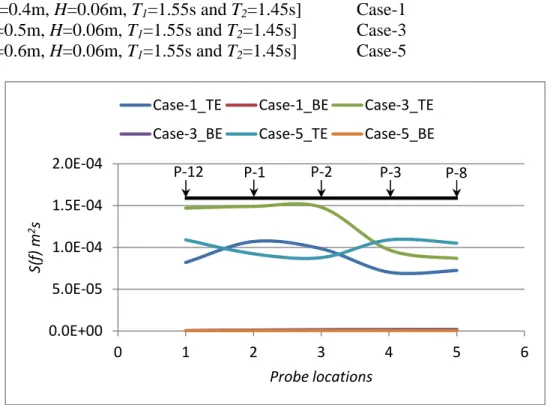
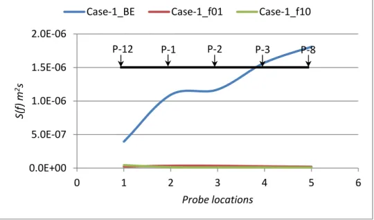
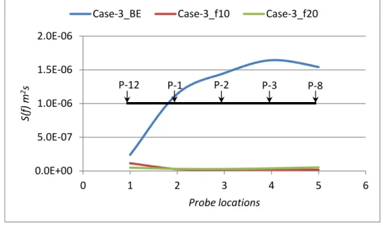
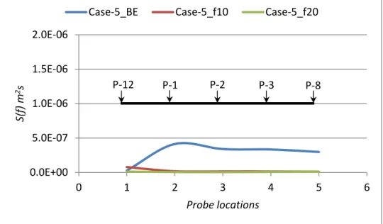
Figs. 20a to 20h show comparisons of the wave energies among Case-1, Case-3 and Case-5. In these three different cases wave periods and wave height remain constant but water depth varies (h=0.4m, 0.5m and 0.6m). The results are shown along the longitudinal probes P-12_P-1_P-2_P-3_P-8 and along the transverse probes P-4_P-3_P-6. Fig. 20a shows the comparisons between the Total Energy (TE) and Bounded Energy (BE) among above three cases along the longitudinal direction of the tank. On the other hand, Fig. 20b shows similar comparisons along the transverse direction. Figs. 20c and 20d show the comparisons among the BE of waves and natural frequency energy components (NE) in the longitudinal and transverse directions for Case-1. Figs. 20e and 20f show similar comparisons among the BE and NE in the longitudinal and transverse directions for Case-3. Figs. 20g and 20h show similar comparisons for Case-5. Figs. 21a to 21h show similar comparisons as described above but for Case-2, Cas-4 and Case-6. In these cases also a different set of constant wave period and wave height is used over varying water depths. Figs. 22a to 22r show similar comparisons of energies between 1 and Case-2, Case-3 and Case-4 and, Case-5 and Case-6. It may be observed from the Figs. 20a to
21h that BE is O(10-4) compare to TE and NE is O(10-6) compare to BE. That is the NE
in the OEB is exceptionally small to be accounted for at least for the cases we considered here. Table 4 to Table 9 show the energies of different undulations in the OEB for different incident wave conditions mentioned in Table 2. Appendix-III illustrates all figures.
5.2 Mono-chromatic waves
In Table-3, Case-8 represents the shallowest mono-chromatic wave. This case is adopted to analyze and understand the wave propagation and required damping time after
12 OCRE-TR-2014-013
the wave making is ended in the tank. Figs. 23a to 34j show the surface elevations for different propagation time segments (0-20s, 8-9.33s, 10-11.33s, 15-16.33s and 18.67-20s) and their corresponding energy spectra for Case-8. The results are shown at probes P-1, P-2, P-3, P-4, P-5, P-6, P-7, P-8, P-9, P-10, P-12 and P-14. Appendix-IV demonstrates above figures.
Figs. 35a to 39d show amplitude spectra of the incident frequencies, different
interacted frequency components (f, 2f, 3f, ….) and wave tank’s natural frequency
components (f01, f10, f02,….) and are normalized by the incident wave height H. Figures
show results for Case-8 at probes P-12_P-1_P-2_P-3_P-8 along the longitudinal direction of the tank for different time segments (0-20s, 10-11.33s, 15-16.33s and 18.67-20s).
Appendix-V shows these figures.
Figs. 40a to 43d show comparisons of the wave energies among cases, Case-7, Case-8 and Case-9. Here Case-7 and Case-8 have similar water depth and similar wave height but different waver periods (T=2.145s and T=4.105s). The results are shown along longitudinal probes P-12_P-1_P-2_P-3_P-8and along the transverse probes P-4_P-3_P-6. Fig. 40a shows the comparisons between the Total Energy (TE) and Bounded Energy (BE) among above three cases along the longitudinal direction of the tank. On the other hand, Fig. 40b shows similar comparisons along the transverse direction. Fig. 40c shows the comparisons among measured natural frequency energy components of the OEB for Case-7, Case-8 and Case-9 at wave probes P-12_P-1_P-2_P-3_P-8. On the other hand, Fig. 40d describes the comparisons among measured natural frequency energy components of the OEB for Case-7, Case-8 and Case-9 at wave probes P-4_P-3_P-6.
Fig. 41a shows measured total wave energy (TE) and natural frequency energy (NE) components of the OEB for Case-7 at wave probes P-12_P-1_P-2_P-3_P-8. On the other hand, Fig. 41b shows the measured total wave energy (TE) and natural frequency energy (NE) components of the OEB for Case-7 at wave probes P-4_P-3_P-6. Figs. 41c and 41d describe only the measured natural frequency energy components of the OEB for Case-7 at wave probes P-12_P-1_P-2_P-3_P-8 and P-4_P-3_P-6, respectively.
Figs. 42a to 42d show similar comparisons as above for Case-8 and Figs. 43a to 43d show comparisons for Case-9.
It may be observed from the Figs. 40a to 43d that NE is O(10-4) compare to TE. So to
speak the NE in the OEB is exceptionally small to be accounted for at least for the cases we considered here. Table 10 to Table 12 show the energies of different undulations in the OEB for different incident wave conditions mentioned in Table 3. Appendix-VI displays all these figures.
6. CONCLUSIONS
Several cases of measured wave data in the OEB for mono- and bi-chromatic shallow water waves are analyzed. For bi-chromatic waves, it is found that the primary frequency components are interacting with each other in different forms. From both the mono- and
OCRE-TR-2014-013 13
bi-chromatic waves, we have observed that the natural frequency components are very small regardless of varying incident wave conditions. In the analyses Case-2 [h=0.4m,
H=0.06m, T1=2.22s and T2=2.0s] and Case-8 [h=0.4m, H=0.08m and T=4.105s] are
watched more closely than any other cases as these two cases are most shallow water cases that we considered here.
It is observed that for most of the mono- and bi-chromatic cases the residual wave
energies are of O(10-4) of the primary wave energies after 8 or 10 minutes the wave
making is terminated. So the traditional waiting times, 20 minutes in between two runs is not necessary for all cases. So NRC can save and earn more money by accommodating more commercial projects. According to FY2013-2014, the savings could be 190.4 hours of OEB time with wave makers (in average of 20% of the total OEB usage, 952 hours). In terms of money this saving has a value of $55K for OGD projects or $100K for external client projects.
From the comparisons it is observed that bounded wave energy is just 0.5% to 2.5% compare to the respective primary wave energy. On the other hand, the energies of different natural frequency components are 0.01% to 0.15% to the generated primary waves. It is also found that the natural frequency energy components in the transverse direction are negligible compare to the longitudinal direction for higher modes. However, the natural frequency energy components in both directions are found too small in magnitude to be taken into account for shallow water waves that we considered here.
REFERENCES
Mansard, E. P. D., Sand, S. E. and Klinting, P.; (1987) Sub- and super-harmonics in
natural waves, Proc. of the 6th OMAE Conf., Houston, TX, USA.
Mei, C.C., 1999: The applied dynamics of ocean surface waves, Advance series on ocean Engineering, Vol. 1, World Scientific, pp 740.
Sand, S. E. and Mansard, E. P. D.; (1986) Reproduction of higher harmonic waves,
National Research Council of Canada, Hydraulic Laboratory, Technical Report
TR-HY-012.
Zaman, M. H., Peng, H., Baddour, E., Spencer, D. and Mckay, S.; (2010): Identifications
of spurious waves in the wave tank with shallow water, Proc. of the 29th Int. Conf. on
offshore Mech. and Arctic Eng. (OMAE-2010), ASME, Shanghai, China, 13 pages, on CD-ROM.
Zaman, M. H., Peng, H., Baddour, E. and McKay, S., 2011: Spurious waves during
generation of multi-chromatic waves in the wave tank in shallow water, 30th Int. Conf. on
offshore Mech. and Arctic Eng. OMAE-2011, The Netherlands, 9 pages, on CD-ROM.
14 OCRE-TR-2014-013
Appendix-1
Surface elevations for different time segments for bi-chromatic waves and their corresponding energy specta for Case-2.
OCRE-TR-2014-013 15
Fig. 2a Measured total surface elevation at P-1. Fig. 2b Energy for total set of data at P-1.
[h=0.4m, H=0.06m, T1=2.22s and T2=2.0s]
Fig. 2c Surface elevation (10-11.33 minutes) data at P-1. Fig. 2d Energy for 10-11.33 minutes data (4096 data used) at P-1.
16 OCRE-TR-2014-013
Fig. 2e Surface elevation (15-16.33 minutes) data at P-1. Fig. 2f Energy for 15-16.33 minutes data (4096 data used) at P-1.
[h=0.4m, H=0.06m, T1=2.22s and T2=2.0s]
Fig. 2g Surface elevation (18.67-20 minutes) data at P-1. Fig. 2h Energy for 18.67-20 minutes data (4096 data used) at P-1.
OCRE-TR-2014-013 17
Fig. 3a Measured total surface elevation at P-2. Fig. 3b Energy for total set of data at P-2.
[h=0.4m, H=0.06m, T1=2.22s and T2=2.0s]
Fig. 3c Surface elevation (10-11.33 minutes) data at P-2. Fig. 3d Energy for 10-11.33 minutes data (4096 data used) at P-2.
18 OCRE-TR-2014-013
Fig. 3e Surface elevation (15-16.33 minutes) data at P-2. Fig. 3f Energy for 15-16.33 minutes data (4096 data used) at P-2.
[h=0.4m, H=0.06m, T1=2.22s and T2=2.0s]
Fig. 3g Surface elevation (18.67-20 minutes) data at P-2. Fig. 3h Energy for 18.67-20 minutes data (4096 data used) at P-2.
OCRE-TR-2014-013 19
Fig. 4a Measured total surface elevation at P-3. Fig. 4b Energy for total set of data at P-3.
[h=0.4m, H=0.06m, T1=2.22s and T2=2.0s]
Fig. 4c Surface elevation (10-11.33 minutes) data at P-3. Fig. 4d Energy for 10-11.33 minutes data (4096 data used) at P-3.
20 OCRE-TR-2014-013
Fig. 4e Surface elevation (15-16.33 minutes) data at P-3. Fig. 4f Energy for 15-16.33 minutes data (4096 data used) at P-3.
[h=0.4m, H=0.06m, T1=2.22s and T2=2.0s]
Fig. 4g Surface elevation (18.67-20 minutes) data at P-3. Fig. 4h Energy for 18.67-20 minutes data (4096 data used) at P-3.
OCRE-TR-2014-013 21
Fig. 5a Measured total surface elevation at P-4. Fig. 5b Energy for total set of data at P-4.
[h=0.4m, H=0.06m, T1=2.22s and T2=2.0s]
Fig. 5c Surface elevation (10-11.33 minutes) data at P-4. Fig. 5d Energy for 10-11.33 minutes data (4096 data used) at P-4.
22 OCRE-TR-2014-013
Fig. 5e Surface elevation (15-16.33 minutes) data at P-4. Fig. 5f Energy for 15-16.33 minutes data (4096 data used) at P-4.
[h=0.4m, H=0.06m, T1=2.22s and T2=2.0s]
Fig. 5g Surface elevation (18.67-20 minutes) data at P-4. Fig. 5h Energy for 18.67-20 minutes data (4096 data used) at P-4.
OCRE-TR-2014-013 23
Fig. 6a Measured total surface elevation at P-5. Fig. 6b Energy for total set of data at P-5.
[h=0.4m, H=0.06m, T1=2.22s and T2=2.0s]
Fig. 6c Surface elevation (10-11.33 minutes) data at P-5. Fig. 6d Energy for 10-11.33 minutes data (4096 data used) at P-5.
24 OCRE-TR-2014-013
Fig. 6e Surface elevation (15-16.33 minutes) data at P-5. Fig. 6f Energy for 15-16.33 minutes data (4096 data used) at P-5.
[h=0.4m, H=0.06m, T1=2.22s and T2=2.0s]
Fig. 6g Surface elevation (18.67-20 minutes) data at P-5. Fig. 6h Energy for 18.67-20 minutes data (4096 data used) at P-5.
OCRE-TR-2014-013 25
Fig. 7a Measured total surface elevation at P-6. Fig. 7b Energy for total set of data at P-6.
[h=0.4m, H=0.06m, T1=2.22s and T2=2.0s]
Fig. 7c Surface elevation (10-11.33 minutes) data at P-6. Fig. 7d Energy for 10-11.33 minutes data (4096 data used) at P-6.
26 OCRE-TR-2014-013
Fig. 7e Surface elevation (15-16.33 minutes) data at P-6. Fig. 7f Energy for 15-16.33 minutes data (4096 data used) at P-6.
[h=0.4m, H=0.06m, T1=2.22s and T2=2.0s]
Fig. 7g Surface elevation (18.67-20 minutes) data at P-6. Fig. 7h Energy for 18.67-20 minutes data (4096 data used) at P-6.
OCRE-TR-2014-013 27
Fig. 8a Measured total surface elevation at P-7. Fig. 8b Energy for total set of data at P-7.
[h=0.4m, H=0.06m, T1=2.22s and T2=2.0s]
Fig. 8c Surface elevation (10-11.33 minutes) data at P-7. Fig. 8d Energy for 10-11.33 minutes data (4096 data used) at P-7.
28 OCRE-TR-2014-013
Fig. 8e Surface elevation (15-16.33 minutes) data at P-7. Fig. 8f Energy for 15-16.33 minutes data (4096 data used) at P-7.
[h=0.4m, H=0.06m, T1=2.22s and T2=2.0s]
Fig. 8g Surface elevation (18.67-20 minutes) data at P-7. Fig. 8h Energy for 18.67-20 minutes data (4096 data used) at P-7.
OCRE-TR-2014-013 29
Fig. 9a Measured total surface elevation at P-8. Fig. 9b Energy for total set of data at P-8.
[h=0.4m, H=0.06m, T1=2.22s and T2=2.0s]
Fig. 9c Surface elevation (10-11.33 minutes) data at P-8. Fig. 9d Energy for 10-11.33 minutes data (4096 data used) at P-8.
30 OCRE-TR-2014-013
Fig. 9e Surface elevation (15-16.33 minutes) data at P-8. Fig. 9f Energy for 15-16.33 minutes data (4096 data used) at P-8.
[h=0.4m, H=0.06m, T1=2.22s and T2=2.0s]
Fig. 9g Surface elevation (18.67-20 minutes) data at P-8. Fig. 9h Energy for 18.67-20 minutes data (4096 data used) at P-8.
OCRE-TR-2014-013 31
Fig. 10a Measured total surface elevation at P-9. Fig. 10b Energy for total set of data at P-9.
[h=0.4m, H=0.06m, T1=2.22s and T2=2.0s]
Fig. 10c Surface elevation (10-11.33 minutes) data at P-9. Fig. 10d Energy for 10-11.33 minutes data (4096 data used) at P-9.
32 OCRE-TR-2014-013
Fig. 10e Surface elevation (15-16.33 minutes) data at P-9. Fig. 10f Energy for 15-16.33 minutes data (4096 data used) at P-9.
[h=0.4m, H=0.06m, T1=2.22s and T2=2.0s]
Fig. 10g Surface elevation (18.67-20 minutes) data at P-9. Fig. 10h Energy for 18.67-20 minutes data (4096 data used) at P-9.
OCRE-TR-2014-013 33
Fig. 11a Measured total surface elevation at P-10. Fig. 11b Energy for total set of data at P-10.
[h=0.4m, H=0.06m, T1=2.22s and T2=2.0s]
Fig. 11c Surface elevation (10-11.33 minutes) data at P-10. Fig. 11d Energy for 10-11.33 minutes data (4096 data used) at P-10.
34 OCRE-TR-2014-013
Fig. 11e Surface elevation (15-16.33 minutes) data at P-10. Fig. 11f Energy for 15-16.33 minutes data (4096 data used) at P-10.
[h=0.4m, H=0.06m, T1=2.22s and T2=2.0s]
Fig. 11g Surface elevation (18.67-20 minutes) data at P-10. Fig. 11h Energy for 18.67-20 minutes data (4096 data used) at P-10.
OCRE-TR-2014-013 35
Fig. 12a Measured total surface elevation at P-12. Fig. 12b Energy for total set of data at P-12.
[h=0.4m, H=0.06m, T1=2.22s and T2=2.0s]
Fig. 12c Surface elevation (10-11.33 minutes) data at P-12. Fig. 12d Energy for 10-11.33 minutes data (4096 data used) at P-12.
36 OCRE-TR-2014-013
Fig. 12e Surface elevation (15-16.33 minutes) data at P-12. Fig. 12f Energy for 15-16.33 minutes data (4096 data used) at P-12.
[h=0.4m, H=0.06m, T1=2.22s and T2=2.0s]
Fig. 12g Surface elevation (18.67-20 minutes) data at P-12. Fig. 12h Energy for 18.67-20 minutes data (4096 data used) at P-12.
OCRE-TR-2014-013 37
Fig. 13a Measured total surface elevation at P-14. Fig. 13b Energy for total set of data at P-14.
[h=0.4m, H=0.06m, T1=2.22s and T2=2.0s] 3.0 2.5 2.0 1.5 1.0 0.5 m m 680s 660 640 620 600 time(seconds)
Fig. 13c Surface elevation (10-11.33 minutes) data at P-14. Fig. 13d Energy for 10-11.33 minutes data (4096 data used) at P-14.
38 OCRE-TR-2014-013 2.4 2.2 2.0 1.8 1.6 1.4 1.2 m m 980s 960 940 920 900 time(seconds)
Fig. 13e Surface elevation (15-16.33 minutes) data at P-14. Fig. 13f Energy for 15-16.33 minutes data (4096 data used) at P-14.
[h=0.4m, H=0.06m, T1=2.22s and T2=2.0s] 2.4 2.2 2.0 1.8 1.6 1.4 1.2 m m 1200s 1180 1160 1140 1120 time(seconds)
Fig. 13g Surface elevation (18.67-20 minutes) data at P-14. Fig. 13h Energy for 18.67-20 minutes data (4096 data used) at P-14.
OCRE-TR-2014-013 39
Appendix-II
Interaction of the primary wave components and natural frequency energy components for Case-2.
40 OCRE-TR-2014-013
Fig. 14a: Probe-12: Full normalized amplitude spectrum, 20 minutes wave data
[h=0.4m, H=0.06m, T1=2.22s and T2=2.0s] 1.0x10⁻¹ 0.8 0.6 0.4 0.2 0.0 a m p lit u d e /H 1.6 1.4 1.2 1.0 0.8 0.6 0.4 0.2 0.0 Hz 40f1-36f2 p18 f20 p33 f01 p46 f30 p50f2-f1p61 2f1-f2 p481 f1 p541 f2 p600 2f2-f1 p660 3f1-f2 p1022 2f1 p1081 f1+f2 p1140 2f2 p1200 2f1+f2 p1681 2f2+f1 p1740
OCRE-TR-2014-013 41
Fig. 14b: Probe-12: Normalized amplitude spectrum after (10-11.320 minutes of) wave making stopped
[h=0.4m, H=0.06m, T1=2.22s and T2=2.0s] 6x10⁻³ 5 4 3 2 1 0 a m p lit u d e /H 10 8 6 4 2 0 Hz f10 p1 f02 p6 f2 p41 3f2-2f1 p49 2f1 p74 2f2 p82 f1+f2 p78 18f2-17f1 p110 f1+2f2 p119 16f1-11f2 p140 15f1-10f2 p144 43f1-35f2 p153 51f2-52f1 p170
42 OCRE-TR-2014-013
Fig. 14c: Probe-12: Normalized amplitude spectrum after [15-16.320 minutes of] wave making stopped
[h=0.4m, H=0.06m, T1=2.22s and T2=2.0s] 6x10⁻³ 5 4 3 2 1 0 a m p lit u d e /H 10 8 6 4 2 0 Hz f10 p1 f02 p6 f2 p41 2f1 p74 2f2 p82 13f1-9f2 p111 19f2-18f1 p114 20f2-19f1 p118 40f1-33f2 p124 5f2-2f1 p131 15f1-10f2 p144
OCRE-TR-2014-013 43
Fig. 14d: Probe-12: Normalized amplitude spectrum after [18.67-20 minutes of] wave making stopped
[h=0.4m, H=0.06m, T1=2.22s and T2=2.0s] 6x10⁻³ 5 4 3 2 1 0 a m p lit u d e /H 10 8 6 4 2 0 Hz f10 p1 29f2-32f1 p7 f1+f2 p78 2f1 p74 13f1-9f2 p111
44 OCRE-TR-2014-013
Fig. 15a: Probe-1: Full spectrum, 20 minutes wave data
[h=0.4m, H=0.06m, T1=2.22s and T2=2.0s] 14 12 10 8 6 4 2 0 s (f )/ a ² 1.6 1.4 1.2 1.0 0.8 0.6 0.4 0.2 0.0 Hz f20 p33 f01 p46 f30 p50 f2-f1 p60 2f1-f2 p479 f1 p540 f2 p601 2f2-f1 p662 3f1-f2 p1020 2f1 p1079 f1+f2 p1141 2f2 p1202 3f1 p1623 2f1+f2 p1681 2f2+f1 p1741 3f2 p1799
OCRE-TR-2014-013 45
Fig. 15b: Probe-1: Spectrum after [10-11.320 minutes of] wave making stopped
[h=0.4m, H=0.06m, T1=2.22s and T2=2.0s] 5x10⁻³ 4 3 2 1 0 s (f )/ a ² 10 8 6 4 2 0 Hz f10 p1 f01 p3 f02 p6 f2 p41 17f1-14f2 p54 2f1 p74 17f2-38f1 p113 78f1-67f2 p134 67f1-70f2 p161 95f1-81f2 p188 53f2-53f1 p215 11f1-4f2 p242 75f1-61f2 p269 8f1+2f2 p377 15f2-5f1 p430 101f2-99f1 p592
46 OCRE-TR-2014-013
Fig. 15c: Probe-1: Spectrum after (15-16.33 minutes of) wave making stopped
[h=0.4m, H=0.06m, T1=2.22s and T2=2.0s] 5x10⁻³ 4 3 2 1 0 s (f )/ a ² 10 8 6 4 2 0 Hz f10 p1 f01 p3 43f2-47f1 p27 17f1-14f2 p54 29f2-30f1 p81 63f2-67f1 p108 6f2-3f1 p135 61f1-51f2 p162 95f1-81f2 p188 53f2-53f1 p215 11f1-4f2 p242 75f1-61f2 p269 8f1+2f2 p377 88f2-86f1 p431 74f2-69f1 p485 56f1-22f2p592 50f2-38f1p646 36f2-21f1p700
OCRE-TR-2014-013 47
Fig. 15d: Probe-1: Spectrum after (18.67-20 minutes of) wave making stopped
[h=0.4m, H=0.06m, T1=2.22s and T2=2.0s] 5x10⁻³ 4 3 2 1 0 s (f )/ a ² 10 8 6 4 2 0 Hz f10 p1 43f2-47f1p27 17f1-14f2 p54 29f2-30f1 p81 63f2-67f1 p108 6f2-3f1 p135 61f1-51f2 p162 35f2-33f1 p216 92f2-97f1 p189 75f1-61f2 p269 8f1+2f2p377 88f2-86f1 p431 74f2-69f1 p485 23f2-8f1 p647 23f1-f2 p808 36f2-21f1 p700
48 OCRE-TR-2014-013
Fig. 16a: Probe-1: Full Normalized amplitude spectrum, 20 minutes wave data
[h=0.4m, H=0.06m, T1=2.22s and T2=2.0s] 100x10-3 80 60 40 20 0 a m p lit u d e /H 1.6 1.4 1.2 1.0 0.8 0.6 0.4 0.2 0.0 Hz f20 p33 f01 p46 f30 p50 f2-f1 p60 2f1-f2 p479 f1 p540 f2 p601 2f2-f1 p662 3f1-f2 p1020 2f1 p1079 f1+f2 p1141 2f2 p1202 3f1 p1623 2f1+f2 p1681 2f2+f1 p1741 3f2 p1799
OCRE-TR-2014-013 49
Fig. 16b: Probe-1: Normalized amplitude spectrum after (10-11.33 minutes of) wave making stopped
[h=0.4m, H=0.06m, T1=2.22s and T2=2.0s] 6x10⁻³ 5 4 3 2 1 0 a m p lit u d e /H 10 8 6 4 2 Hz f10 p1 f01 p3 f02 p6 f2 p41 17f1-14f2 p54 2f1 p74 17f2-38f1 p113 78f1-67f2 p134 67f1-70f2 p161 95f1-81f2 p188 53f2-53f1 p215 11f1-4f2 p242 75f1-61f2 p269 8f1+2f2 p377 15f2-5f1 p430 101f2-99f1 p592
50 OCRE-TR-2014-013
Fig. 16c: Probe-1: Normalized amplitude spectrum after (15-16.33 minutes of) wave making stopped
[h=0.4m, H=0.06m, T1=2.22s and T2=2.0s] 6x10⁻³ 5 4 3 2 1 0 a m p lit u d e /H 10 8 6 4 2 0 Hz f10 p1 f01 p3 43f2-47f1 p27 17f1-14f2 p54 29f2-30f1 p81 63f2-67f1 p108 6f2-3f1 p135 61f1-51f2 p162 53f2-53f1 p215 95f1-81f2 p188 11f1-4f2 p242 75f1-61f2 p269 8f1+2f2 p377 88f2-86f1 p431 74f2-69f1 p485 56f1-22f2 p592 50f2-38f1 p646 36f2-21f1 p700
OCRE-TR-2014-013 51
Fig. 16d: Probe-1: Normalized amplitude spectrum after (18.67-20 minutes of) wave making stopped
[h=0.4m, H=0.06m, T1=2.22s and T2=2.0s] 6x10⁻³ 5 4 3 2 1 0 a m p lit u d e /H 10 8 6 4 2 0 Hz f10 p1 43f2-47f1 p27 17f1-14f2 p54 29f2-30f1 p81 63f2-67f1 p108 6f2-3f1 p135 61f1-51f2 p162 35f2-33f1 p216 92f2-97f1 p189 75f1-61f2 p269 8f1+2f2 p377 88f2-86f1 p431 74f2-69f1 p485 23f2-8f1 p647 36f2-21f1p700 23f1-f2 p808
52 OCRE-TR-2014-013
Fig. 17a: Probe-2: Normalized amplitude spectrum, 20 minutes wave data
[h=0.4m, H=0.06m, T1=2.22s and T2=2.0s] 100x10-3 80 60 40 20 0 a m p lit u d e /H 1.6 1.4 1.2 1.0 0.8 0.6 0.4 0.2 0.0 Hz f20 p33 f01 p46 f30 p50 f2-f1 p60 2f1-f2 p479 f1 p541 f2 p600 2f2-f1 p662 3f1-f2 p1020 2f1 p1079 f1+f2 p1141 2f2 p1199 3f1 p1620 2f1+f2 p1678 2f2+f1 p1738 3f2 p1802
OCRE-TR-2014-013 53
Fig. 17b: Probe-2: Normalized amplitude spectrum after (10-11.33 minutes of) wave making stopped
[h=0.4m, H=0.06m, T1=2.22s and T2=2.0s] 6x10⁻³ 5 4 3 2 1 0 a m p lit u d e /H 10 8 6 4 2 0 Hz f10 p1 f01 p3 f02 p6 43f2-47f1 p27 f2 p41 17f1-14f2 p54 29f2-30f1 p81 19f2-18f1 p114 78f1-67f2 p134 67f2-70f1 p161 95f1-81f2 p188 53f2-53f1 p215 11f1-4f2 p242 75f1-61f2 p269 25f2-19f1 p323 8f1+2f2 p377 68f2-66f1 p350 42f1-28f2 p403 15f2-5f1 p430 58f2-52f1 p457 101f2-99f1 p484 56f1-36f2 p592 50f2-38f1 p646 54f2-41f1p699 23f1-3f2 p726 35f2-17f1 p807
54 OCRE-TR-2014-013
Fig. 17c: Probe-2: Normalized amplitude spectrum after (15-16.33 minutes of) wave making stopped
[h=0.4m, H=0.06m, T1=2.22s and T2=2.0s] 6x10⁻³ 5 4 3 2 1 0 a m p lit u d e /H 10 8 6 4 2 0 Hz f10 p1 f02 p6 f01 p3 43f2-47f1 p27 17f1-14f2 p54 29f2-30f1 p81 63f2-67f1 p108 6f2-3f1 p135 61f1-51f2 p162 19f2-16f1 p188 53f2-53f1 p215 11f1-4f2 p242 75f1-61f2 p269 28f1-18f2 p296 25f2-19f1 p323 68f2-66f1 p350 8f1+2f2 p377 72f1-55f2 p404 88f2-86f1 p431 89f1-69f2 p458 74f2-69f1 p485 44f2-35f1 p511 39f1-22f2 p538 56f1-22f2 p592 50f2-38f1 p646 36f2-21f1p700 70f2-58f1 p727 23f1-f2 p808
OCRE-TR-2014-013 55
Fig. 17d: Probe-2: Normalized amplitude spectrum after (18.67-20 minutes of) wave making stopped
[h=0.4m, H=0.06m, T1=2.22s and T2=2.0s] 6x10⁻³ 5 4 3 2 1 0 a m p lit u d e /H 10 8 6 4 2 0 Hz f10 p1 43f2-47f1 p27 17f1-14f2 p54 29f2-30f1 p81 63f2-67f1 p108 6f2-3f1 p135 61f1-51f2 p162 92f2-97f1 p189 35f2-33f1 p216 11f1-4f2 p242 75f1-61f2 p269 28f1-18f2 p296 25f2-19f1 p323 68f2-66f1 p350 8f1+2f2 p377 72f1-55f2 p404 88f2-86f1 p431 89f1-69f2 p458 74f2-69f1 p485 17f2-5f1 p512 60f2-52f1 p539 86f1-63f2 p593 23f2-8f1 p647 36f2-21f1 p700 23f1-f2p808
56 OCRE-TR-2014-013
Fig. 18a: Probe-3: Normalized amplitude spectrum, 20 minutes wave data
[h=0.4m, H=0.06m, T1=2.22s and T2=2.0s] 1.0x10⁻¹ 0.8 0.6 0.4 0.2 0.0 a m p lit u d e /H 1.6 1.4 1.2 1.0 0.8 0.6 0.4 0.2 0.0 Hz f20 p33 f01 p46 f30 p50 f2-f1 p60 2f1-f2p479 f1 p540 f2 p600 2f2-f1 p662 3f1-f2 p1021 2f1 p1079 f1+f2 p1140 2f2 p1201 3f1 p1618 2f1+f2 p1682 2f2+f1 p17383f2 p1804
OCRE-TR-2014-013 57
Fig. 18b: Probe-3: Normalized amplitude spectrum after (10-11.33 minutes of) wave making stopped
[h=0.4m, H=0.06m, T1=2.22s and T2=2.0s] 6x10⁻³ 5 4 3 2 1 0 a m p lit u d e /H 10 8 6 4 2 0 Hz f10 p1 f01 p3 f02 p6 f2 p41 29f1-25f2 p46 14f1-11f2 p66 f1+f2 p78 2f2 p82 15f1-11f2 p103 f1+2f2 p119 12f1-8f2 p115 32f2-32f1 p130 19f2-17f1 p151 3f1 p111
58 OCRE-TR-2014-013
Fig. 18d: Probe-3: Normalized amplitude spectrum after (18.67-20 minutes of) wave making stopped
[h=0.4m, H=0.06m, T1=2.22s and T2=2.0s] 6x10⁻³ 5 4 3 2 1 0 a m p lit u d e /H 10 8 6 4 2 0 Hz f10 p1 27f1-24f2 p13 f1 p37 17f2-17f1 p69 f1+f2 p78 2f2 p83 18f2-17f1 p110 44f1-36f2 p149 66f2-66f1 p268 67f2-65f1 p346 25f2-9f1 p692
OCRE-TR-2014-013 59
Fig. 19a: Probe-8: Normalized amplitude spectrum, 20 minutes wave data
[h=0.4m, H=0.06m, T1=2.22s and T2=2.0s] 1.0x10⁻¹ 0.8 0.6 0.4 0.2 0.0 a m p lit u d e /H 1.6 1.4 1.2 1.0 0.8 0.6 0.4 0.2 0.0 Hz f20 p33 f01 p46 f30 p50 f2-f1 p60 2f1-f2 p479 f1 p540 f2 p600 2f2-f1 p662 3f1-f2 p1019 2f1 p1078 f1+f2 p1140 2f2 p1203 3f1 p1621 2f1+f2 p1678 2f2+f1 p1737
60 OCRE-TR-2014-013
Fig. 19b: Probe-8: Normalized amplitude spectrum after (10-11.33 minutes of) wave making stopped
[h=0.4m, H=0.06m, T1=2.22s and T2=2.0s] 6x10⁻³ 5 4 3 2 1 a m p lit u d e /H 2.0 1.5 1.0 0.5 0.0 Hz 29f2-31f1 p11 46f2-49f1 p19 33f1-27f2 p28 15f1-10f2 p36 12f1-7f2 p39
OCRE-TR-2014-013 61
Fig. 19c: Probe-8: Normalized amplitude spectrum after (15-16.33 minutes of) wave making stopped
[h=0.4m, H=0.06m, T1=2.22s and T2=2.0s] 6x10⁻³ 5 4 3 2 1 a m p lit u d e /H 2.0 1.5 1.0 0.5 0.0 Hz 29f2-31f1 p11 46f2-49f1 p19 33f1-27f2 p28 31f1-25f2 p30 15f1-10f2 p36
62 OCRE-TR-2014-013
Fig. 19d: Probe-8: Normalized amplitude spectrum after (18.67-20 minutes of) wave making stopped
[h=0.4m, H=0.06m, T1=2.22s and T2=2.0s] 6x10⁻³ 5 4 3 2 1 a m p lit u d e /H 2.0 1.5 1.0 0.5 0.0 Hz 46f2-49f1 p19 32f1-26f2 p29
OCRE-TR-2014-013 63
Appendix-III
Comparisons of Total Energy (TE), Bounded Energy (BE) and Natural frequency Energy components in the tank for Bi-chromatic wave cases (Case-1 to Case-6).
[h=0.4m, H=0.06m, T1=1.55s and T2=1.45s] Case-1 [h=0.5m, H=0.06m, T1=1.55s and T2=1.45s] Case-3 [h=0.6m, H=0.06m, T1=1.55s and T2=1.45s] Case-5 [h=0.4m, H=0.06m, T1=2.22s and T2=2.0s] Case-2 [h=0.5m, H=0.06m, T1=2.22s and T2=2.0s] Case-4 [h=0.6m, H=0.06m, T1=2.22s and T2=2.0s] Case-6
64 OCRE-TR-2014-013 [h=0.4m, H=0.06m, T1=1.55s and T2=1.45s] Case-1 [h=0.5m, H=0.06m, T1=1.55s and T2=1.45s] Case-3 [h=0.6m, H=0.06m, T1=1.55s and T2=1.45s] Case-5
Fig. 20a Measured total (TE) and bounded wave energies (BE) for Case-1, Case-3 and Case-5 at wave probes 12-1-2-3-8.
Fig. 20b Measured total (TE) and bounded wave energies (BE) for Case-1, 3 and 5 at wave probes 4-3-6. 0.0E+00 5.0E‐05 1.0E‐04 1.5E‐04 2.0E‐04 0 1 2 3 4 5 6 S(f ) m 2s Probe locations
Case‐1_TE Case‐1_BE Case‐3_TE Case‐3_BE Case‐5_TE Case‐5_BE
0.0E+00 5.0E‐05 1.0E‐04 1.5E‐04 2.0E‐04 0 1 2 3 4 S( f) m 2s Probe locations
Case‐1_TE Case‐1_BE Case‐3_TE Case‐3_BE Case‐5_TE Case‐5_BE
P‐3 P‐8
P‐12 P‐1 P‐2
OCRE-TR-2014-013 65
Fig. 20c Measured bounded wave (BE) and natural frequency energy components of the OEB for Case-1 at wave probes 12-1-2-3-8.
Fig. 20d Measured bounded wave (BE) and natural frequency energy components (f01, f10) of the
OEB for Case-1 at wave probes 4-3-6.
0.0E+00 5.0E‐07 1.0E‐06 1.5E‐06 2.0E‐06 0 1 2 3 4 5 6 S(f ) m 2s Probe locations
Case‐1_BE Case‐1_f01 Case‐1_f10
0.0E+00 5.0E‐07 1.0E‐06 1.5E‐06 2.0E‐06 0 1 2 3 4 S(f ) m 2s Probe locations
Case‐1_BE Case‐1_f01 Case‐1_f10
P‐3 P‐8
P‐12 P‐1 P‐2
66 OCRE-TR-2014-013
Fig. 20e Measured bounded wave (BE) and natural frequency energy components (f10, f20) of the
OEB for Case-3 at wave probes 12-1-2-3-8.
Fig. 20f Measured bounded wave (BE) and natural frequency energy components (f10, f20) of the
OEB for Case-3 at wave probes 4-3-6.
0.0E+00 5.0E‐07 1.0E‐06 1.5E‐06 2.0E‐06 0 1 2 3 4 5 6 S( f) m 2s Probe locations
Case‐3_BE Case‐3_f10 Case‐3_f20
0.0E+00 5.0E‐07 1.0E‐06 1.5E‐06 2.0E‐06 0 1 2 3 4 S( f) m 2s Probe locations
Case‐3_BE Case‐3_f10 Case‐3_f20
P‐3 P‐8
P‐12 P‐1 P‐2
OCRE-TR-2014-013 67
Fig. 20g Measured bounded wave (BE) and natural frequency energy components (f10, f20) of the
OEB for Case-5 at wave probes 12-1-2-3-8.
Fig. 20h Measured bounded wave (BE) and natural frequency energy components (f10, f20) of the
OEB for Case-5 at wave probes 4-3-6.
0.0E+00 5.0E‐07 1.0E‐06 1.5E‐06 2.0E‐06 0 1 2 3 4 5 6 S( f) m 2s Probe locations
Case‐5_BE Case‐5_f10 Case‐5_f20
0.0E+00 5.0E‐07 1.0E‐06 1.5E‐06 2.0E‐06 0 1 2 3 4 S( f) m 2s Probe locations
Case‐5_BE Case‐5_f10 Case‐5_f20
P‐3 P‐8
P‐12 P‐1 P‐2
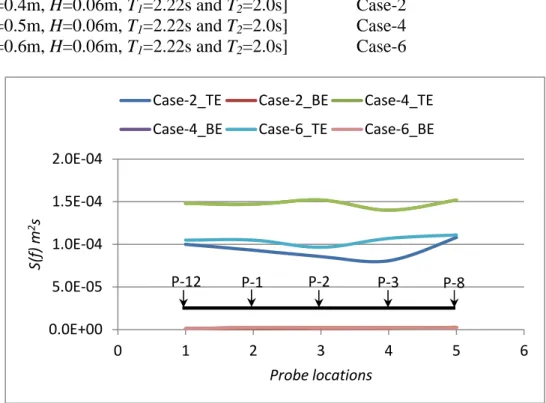
68 OCRE-TR-2014-013 [h=0.4m, H=0.06m, T1=2.22s and T2=2.0s] Case-2 [h=0.5m, H=0.06m, T1=2.22s and T2=2.0s] Case-4 [h=0.6m, H=0.06m, T1=2.22s and T2=2.0s] Case-6
Fig. 21a Measured total (TE) and bounded wave energies (BE) for Case-2, Case-4 and Case-6 at wave probes 12-1-2-3-8.
Fig. 21b Measured total (TE) and bounded wave energies (BE) for Case-2, 4 and 6 at wave probes 4-3-6. 0.0E+00 5.0E‐05 1.0E‐04 1.5E‐04 2.0E‐04 0 1 2 3 4 5 6 S(f ) m 2s Probe locations
Case‐2_TE Case‐2_BE Case‐4_TE Case‐4_BE Case‐6_TE Case‐6_BE
0.0E+00 5.0E‐05 1.0E‐04 1.5E‐04 2.0E‐04 0 1 2 3 4 S(f ) m 2s Probe locations
Case‐2_TE Case‐2_BE Case‐4_TE Case‐4_BE Case‐6_TE Case‐6_BE
P‐3 P‐8
P‐12 P‐1 P‐2
OCRE-TR-2014-013 69
Fig. 21c Measured bounded wave (BE) and natural frequency energy components (f01, f10, f20, f30)
of the OEB for Case-2 at wave probes 12-1-2-3-8.
Fig. 21d Measured bounded wave (BE) and natural frequency energy components (f01, f10, f20, f30)
of the OEB for Case-2 at wave probes 4-3-6.
0.0E+00 1.0E‐06 2.0E‐06 3.0E‐06 0 1 2 3 4 5 6 S(f ) m 2s Probe locations
Case‐2_BE Case‐2_f01 Case‐2_f10 Case‐2_f20 Case‐2_f30 0.0E+00 1.0E‐06 2.0E‐06 3.0E‐06 0 1 2 3 4 S( f) m 2s Probe locations
Case‐2_BE Cas2‐2_f01 Case‐2_f10 Case‐2_f20 Case‐2_f30 P‐3 P‐8
P‐12 P‐1 P‐2
70 OCRE-TR-2014-013
Fig. 21e Measured bounded wave (BE) and natural frequency energy components of the OEB for Case-4 at wave probes 12-1-2-3-8.
Fig. 21f Measured bounded wave (BE) and natural frequency energy components of the OEB for Case-4 at wave probes 4-3-6.
0.0E+00 1.0E‐06 2.0E‐06 3.0E‐06 0 1 2 3 4 5 6 S( f) m 2s Probe locations
Case‐4_BE Case‐4_f01 Case‐4_f20
0.0E+00 1.0E‐06 2.0E‐06 3.0E‐06 0 1 2 3 4 5 S( f) m 2s Probe locations
Case‐4_BE Case‐4_f01 Case‐4_f20
P‐3 P‐8
P‐12 P‐1 P‐2
OCRE-TR-2014-013 71
Fig. 21g Measured bounded wave (BE) and natural frequency energy components (f10, f20) of the
OEB for Case-6 at wave probes 12-1-2-3-8.
Fig. 21h Measured bounded wave (BE) and natural frequency energy components (f01, f10, f20) of
the OEB for Case-6 at wave probes 4-3-6.
0.0E+00 1.0E‐06 2.0E‐06 3.0E‐06 0 1 2 3 4 5 6 S(f) m 2s Probe locations
Case‐6_BE Case‐6_f10 Case‐6_f20
0.0E+00 1.0E‐06 2.0E‐06 3.0E‐06 0 1 2 3 4 5 S(f ) m 2s Probe locations
Case‐6_BE Case‐6_f01 Case‐6_f10 Case‐6_f20
P‐3 P‐8
P‐12 P‐1 P‐2
72 OCRE-TR-2014-013 [h=0.4m, H=0.06m, T1=1.55s and T2=1.45s] Case-1 [h=0.4m, H=0.06m, T1=2.22s and T2=2.0s] Case-2 [h=0.5m, H=0.06m, T1=1.55s and T2=1.45s] Case-3 [h=0.5m, H=0.06m, T1=2.22s and T2=2.0s] Case-4 [h=0.6m, H=0.06m, T1=1.55s and T2=1.45s] Case-5 [h=0.6m, H=0.06m, T1=2.22s and T2=2.0s] Case-6
Fig. 22a Comparisons of measured total (TE) and bounded wave energies (BE) for Case-1 and Case-2 at wave probes 12-1-2-3-8.
Fig. 22b Comparisons of measured total (TE) and bounded wave energies (BE) for Case-1 and Case-2 at wave probes 4-3-6.
0.0E+00 5.0E‐05 1.0E‐04 1.5E‐04 2.0E‐04 0 1 2 3 4 5 6 S(f ) m 2s Probe locations
Case‐1_TE Case‐1_BE Case‐2_TE Case‐2_BE
0.0E+00 5.0E‐05 1.0E‐04 1.5E‐04 2.0E‐04 0 1 2 3 4 S(f ) m 2s Probe locations
Case‐1_TE Case‐1_BE Case‐2_TE Case‐2_BE
P‐3 P‐8
P‐12 P‐1 P‐2
OCRE-TR-2014-013 73
Fig. 22c Comparisons of measured total (TE) and bounded wave energies (BE) for Case-3 and Case-4 at wave probes 12-1-2-3-8.
Fig. 22d Comparisons of measured total (TE) and bounded wave energies (BE) for Case-3 and Case-4 at wave probes 4-3-6.
0.0E+00 5.0E‐05 1.0E‐04 1.5E‐04 2.0E‐04 0 1 2 3 4 5 6 S( f) m 2s Probe locations
Case‐3_TE Case‐3_BE Case‐4_TE Case‐4_BE
0.0E+00 5.0E‐05 1.0E‐04 1.5E‐04 2.0E‐04 0 1 2 3 4 5 S( f) m 2s Probe locations
Case‐3_TE Case‐3_BE Case‐4_TE Case‐4_BE
P‐3 P‐8
P‐12 P‐1 P‐2
74 OCRE-TR-2014-013
Fig. 22e Comparisons of measured total (TE) and bounded wave energies (BE) for Case-5 and Case-6 at wave probes 12-1-2-3-8.
Fig. 22f Comparisons of measured total (TE) and bounded wave energies (BE) for Case-5 and Case-6 at wave probes 4-3-6.
0.0E+00 5.0E‐05 1.0E‐04 1.5E‐04 2.0E‐04 0 1 2 3 4 5 6 S( f) m 2s Probe locations
Case‐5_TE Case‐5_BE Case‐6_TE Case‐6_BE
0.0E+00 5.0E‐05 1.0E‐04 1.5E‐04 2.0E‐04 0 1 2 3 4 S(f ) m 2s Probe locations
Case‐5_TE Case‐5_BE Case‐6_TE Case‐6_BE
P‐3 P‐8
P‐12 P‐1 P‐2
OCRE-TR-2014-013 75
Fig. 22g Comparisons of bounded wave energies (BE) with OEB natural frequency components
(f01, f10, f20, f30) for Case-1 and Case-2 at wave probes 12-1-2-3-8.
Fig. 22h Comparisons of bounded wave energies (BE) with OEB natural frequency components
(f01, f10, f20, f30) for Case-1 and Case-2 at wave probes 4-3-6.
0.0E+00 1.0E‐06 2.0E‐06 3.0E‐06 4.0E‐06 0 1 2 3 4 5 6 S(f ) m 2s Probe locations
Case‐1_BE Case‐1_f01 Case‐1_f10 Case‐2_BE Case‐2_f01 Case‐2_f10 Case‐2_f20 Case‐2_f30
0.0E+00 1.0E‐06 2.0E‐06 3.0E‐06 4.0E‐06 0 1 2 3 4 S(f ) m 2s Probe locations
Case‐1_BE Case‐1_f01 Case‐1_f10 Case‐2_BE Case‐2_f01 Case‐2_f10 Case‐2_f20 Case‐2_f30
P‐3 P‐8
P‐12 P‐1 P‐2
76 OCRE-TR-2014-013
Fig. 22i Comparisons of bounded wave energies (BE) with OEB natural frequency components
(f01, f10, f20) for Case-3 and Case-4 at wave probes 12-1-2-3-8.
Fig. 22j Comparisons of bounded wave energies (BE) with OEB natural frequency components
(f10, f20) for Case-3 and Case-4 at wave probes 4-3-6.
0.0E+00 1.0E‐06 2.0E‐06 3.0E‐06 4.0E‐06 0 1 2 3 4 5 6 S(f ) m 2s Probe locations
Case‐3_BE Case‐3_f10 Case‐3_f20 Case‐4_BE Case‐4_f01 Case‐4_f20
0.0E+00 1.0E‐06 2.0E‐06 3.0E‐06 4.0E‐06 0 1 2 3 4 5 S(f ) m 2s Probe locations
Case‐3_BE Case‐3_f10 Case‐3_f20 Case‐4_BE Case‐4_f01 Case‐4_f20
P‐3 P‐8
P‐12 P‐1 P‐2
OCRE-TR-2014-013 77
Fig. 22k Comparisons of bounded wave energies (BE) with OEB natural frequency components (f10, f20) for Case-5 and Case-6 at wave probes 12-1-2-3-8.
Fig. 22l Comparisons of bounded wave energies (BE) with OEB natural frequency components
( f10, f20) for Case-5 and Case-6 at wave probes 4-3-6.
0.0E+00 1.0E‐06 2.0E‐06 3.0E‐06 4.0E‐06 0 1 2 3 4 5 6 S( f) m 2s Probe locations
Case‐5_BE Case‐5_f10 Case‐5_f20 Case‐6_BE Case‐6_f10 Case‐6_f20
0.0E+00 1.0E‐06 2.0E‐06 3.0E‐06 4.0E‐06 0 1 2 3 4 S( f) m 2s Probe locations
Case‐5_BE Case‐5_f10 Case‐5_f20 Case‐6_BE Case‐6_f10 Case‐6_f20
P‐3 P‐8
P‐12 P‐1 P‐2
78 OCRE-TR-2014-013
Fig. 22m Comparisons of OEB natural frequency components (f01, f10, f20, f30) for Case-1 and
Case-2 at wave probes 12-1-2-3-8.
Fig. 22n Comparisons of OEB natural frequency components (f01, f10, f20, f30) for Case-1 and
Case-2 at wave probes 4-3-6.
0.0E+00 5.0E‐08 1.0E‐07 1.5E‐07 0 1 2 3 4 5 6 S(f ) m 2s Probe locations
Case‐1_f01 Case‐1_f10 Case‐2_f01 Case‐2_f10 Case‐2_f20 Case‐2_f30
0.0E+00 5.0E‐08 1.0E‐07 1.5E‐07 0 1 2 3 4 S( f) m 2s Probe locations
Case‐1_f01 Case‐1_f10 Case‐2_f01 Case‐2_f10 Case‐2_f20 Case‐2_f30
P‐3 P‐8
P‐12 P‐1 P‐2
OCRE-TR-2014-013 79
Fig. 22o Comparisons of OEB natural frequency components (f01, f10, f20) for Case-3 and Case-4
at wave probes 12-1-2-3-8.
Fig. 22p Comparisons of OEB natural frequency components (f01, f10, f20) for Case-3 and Case-4
at wave probes 4-3-6. 0.0E+00 5.0E‐08 1.0E‐07 1.5E‐07 2.0E‐07 0 1 2 3 4 5 6 S( f) m 2s Probe locations
Case‐3_f10 Case‐3_f20 Case‐4_f01 Case‐4_f20
0.0E+00 5.0E‐08 1.0E‐07 1.5E‐07 2.0E‐07 0 1 2 3 4 S( f) m 2s Probe locations
Case‐3_f10 Case‐3_f20 Case‐4_f01 Case‐4_f20 P‐3 P‐8
P‐12 P‐1 P‐2
80 OCRE-TR-2014-013
Fig. 22q Comparisons of OEB natural frequency components (f01, f10, f20) for Case-5 and Case-6
at wave probes 12-1-2-3-8.
Fig. 22r Comparisons of OEB natural frequency components (f01, f10, f20) for Case-5 and Case-6
at wave probes 4-3-6. 0.0E+00 2.0E‐08 4.0E‐08 6.0E‐08 8.0E‐08 1.0E‐07 0 1 2 3 4 5 6 S( f) m 2s Probe locations
Case‐5_f10 Case‐5_f20 Case‐6_f10 Case‐6_f20
0.0E+00 5.0E‐09 1.0E‐08 1.5E‐08 2.0E‐08 0 1 2 3 4 S(f ) m 2s Probe locations
Case‐5_f10 Case‐5_f20 Case‐6_f10 Case‐6_f20 P‐3 P‐8
P‐12 P‐1 P‐2
OCRE-TR-2014-013 81
Appendix-IV
Surface elevations for different time segments for bi-chromatic waves and their corresponding energy specta for Case-8.
82 OCRE-TR-2014-013 80 60 40 20 0 -20 -40 m m 1200s 1000 800 600 400 200 0 time(seconds) 6x10⁻³ 5 4 3 2 1 0 S (f ) (m 2 /H z ) 2.0 1.5 1.0 0.5 0.0 Hz
Fig. 23a Measured total surface elevation at P-1. Fig. 23b Energy for total set of data at P-1.
[h=0.4m, H=0.08m and T=4.105s] -4 -2 0 2 4 m m 560s 540 520 500 480 time(seconds) 800x10-9 600 400 200 0 S (f ) (m 2 /H z ) 2.0 1.5 1.0 0.5 0.0 Hz
Fig. 23c Surface elevation (8-9.33 minutes) data at P-1. Fig. 23d Energy for 8-9.33 minutes data (4096 data used) at P-1.
OCRE-TR-2014-013 83 -4 -2 0 2 4 m m 680s 660 640 620 600 time(seconds) 800x10-9 600 400 200 0 S (f ) (m 2 /H z ) 2.0 1.5 1.0 0.5 0.0 Hz
Fig. 23e Surface elevation (10-11.33 minutes) data at P-1. Fig. 23f Energy for 10-11.33 minutes data (4096 data used) at P-1.
[h=0.4m, H=0.08m and T=4.105s] -4 -2 0 2 4 m m 980s 960 940 920 900 time(seconds) 800x10-9 600 400 200 0 S (f ) (m 2 /H z ) 2.0 1.5 1.0 0.5 0.0 Hz
Fig. 23g Surface elevation (15-16.33 minutes) data at P-1. Fig. 23h Energy for 15-16.33 minutes data (4096 data used) at P-1.
84 OCRE-TR-2014-013 -4 -2 0 2 4 m m 1200s 1180 1160 1140 1120 time(seconds) 800x10-9 600 400 200 0 S (f ) (m 2 /H z ) 2.0 1.5 1.0 0.5 0.0 Hz
Fig. 23i Surface elevation (18.67-20 minutes) data at P-1. Fig. 23j Energy for 18.67-20 minutes data (4096 data used) at P-1.
[h=0.4m, H=0.08m and T=4.105s] 80 60 40 20 0 -20 -40 m m 1200s 1000 800 600 400 200 0 time(seconds) 6x10⁻³ 5 4 3 2 1 0 S (f ) (m 2 /H z ) 2.0 1.5 1.0 0.5 0.0 Hz
Fig. 24a Measured total surface elevation at P-2. Fig. 24b Energy for total set of data at P-2.
OCRE-TR-2014-013 85 -4 -2 0 2 4 m m 560s 540 520 500 480 time(seconds) 800x10-9 600 400 200 0 S (f ) (m 2 /H z ) 2.0 1.5 1.0 0.5 0.0 Hz
Fig. 24c Surface elevation (8-9.33 minutes) data at P-2. Fig. 24d Energy for 8-9.33 minutes data (4096 data used) at P-2
[h=0.4m, H=0.08m and T=4.105s] -4 -2 0 2 4 m m 680s 660 640 620 600 time(seconds) 800x10-9 600 400 200 0 S (f ) (m 2 /H z ) 2.0 1.5 1.0 0.5 0.0 Hz
Fig. 24e Surface elevation (10-11.33 minutes) data at P-2. Fig. 24f Energy for 10-11.33 minutes data (4096 data used) at P-2.
86 OCRE-TR-2014-013 -4 -2 0 2 4 m m 980s 960 940 920 900 time(seconds) 800x10-9 600 400 200 0 S (f ) (m 2 /H z ) 2.0 1.5 1.0 0.5 0.0 Hz
Fig. 24g Surface elevation (15-16.33 minutes) data at P-2. Fig. 24h Energy for 15-16.33 minutes data (4096 data used) at P-2.
[h=0.4m, H=0.08m and T=4.105s] -4 -2 0 2 4 m m 1200s 1180 1160 1140 1120 time(seconds) 800x10-9 600 400 200 0 S (f ) (m 2 /H z ) 2.0 1.5 1.0 0.5 0.0 Hz
Fig. 24i Surface elevation (18.67-20 minutes) data at P-2. Fig. 24j Energy for 18.67-20 minutes data (4096 data used) at P-2.
OCRE-TR-2014-013 87 80 60 40 20 0 -20 -40 m m 1200s 1000 800 600 400 200 0 time(seconds) 6x10⁻³ 5 4 3 2 1 0 S (f ) (m 2 /H z ) 2.0 1.5 1.0 0.5 0.0 Hz
Fig. 25a Measured total surface elevation at P-3. Fig. 25b Energy for total set of data at P-3.
[h=0.4m, H=0.08m and T=4.105s] -4 -2 0 2 4 m m 560s 540 520 500 480 time(seconds) 800x10-9 600 400 200 0 S (f ) (m 2 /H z ) 2.0 1.5 1.0 0.5 0.0 Hz
Fig. 25c Surface elevation (8-9.33 minutes) data at P-3. Fig. 25d Energy for 8-9.33 minutes data (4096 data used) at P-3
88 OCRE-TR-2014-013 -4 -2 0 2 4 m m 680s 660 640 620 600 time(seconds) 800x10-9 600 400 200 0 S (f ) (m 2 /H z ) 2.0 1.5 1.0 0.5 0.0 Hz
Fig. 25e Surface elevation (10-11.33 minutes) data at P-3. Fig. 25f Energy for 10-11.33 minutes data (4096 data used) at P-3.
[h=0.4m, H=0.08m and T=4.105s] -4 -2 0 2 4 m m 980s 960 940 920 900 time(seconds) 800x10-9 600 400 200 0 S (f ) (m 2 /H z ) 2.0 1.5 1.0 0.5 0.0 Hz
Fig. 25g Surface elevation (15-16.33 minutes) data at P-3. Fig. 25h Energy for 15-16.33 minutes data (4096 data used) at P-3.
OCRE-TR-2014-013 89 -4 -2 0 2 4 m m 1200s 1180 1160 1140 1120 time(seconds) 800x10-9 600 400 200 0 S (f ) (m 2 /H z ) 2.0 1.5 1.0 0.5 0.0 Hz
Fig. 25i Surface elevation (18.67-20 minutes) data at P-3. Fig. 25j Energy for 18.67-20 minutes data (4096 data used) at P-3.
[h=0.4m, H=0.08m and T=4.105s] 80 60 40 20 0 -20 -40 m m 1200s 1000 800 600 400 200 0 time(seconds) 6x10⁻³ 5 4 3 2 1 0 S (f ) (m 2 /H z ) 2.0 1.5 1.0 0.5 0.0 Hz
Fig. 26a Measured total surface elevation at P-4. Fig. 26b Energy for total set of data at P-4.
![Fig. 14a: Probe-12: Full normalized amplitude spectrum, 20 minutes wave data [h=0.4m, H=0.06m, T 1 =2.22s and T 2 =2.0s] 1.0x10-10.80.60.40.20.0amplitude/H 1.61.41.21.00.80.60.40.20.0Hz40f1-36f2p18f20p33f01p46f30p50f2-f1p612f1-f2p481f1p541f2p6002f2-f1p660](https://thumb-eu.123doks.com/thumbv2/123doknet/14103079.465821/46.1188.111.1066.122.711/fig-probe-normalized-amplitude-spectrum-minutes-wave-amplitude.webp)
![Fig. 16a: Probe-1: Full Normalized amplitude spectrum, 20 minutes wave data [h=0.4m, H=0.06m, T 1 =2.22s and T 2 =2.0s] 100x10-3806040200amplitude/H 1.61.41.21.00.80.60.40.20.0Hzf20p33f01p46f30p50f2-f1p602f1-f2p479f1p540f2p6012f2-f1p6623f1-f2p10202f1p1079](https://thumb-eu.123doks.com/thumbv2/123doknet/14103079.465821/54.1188.108.1065.110.679/fig-probe-normalized-amplitude-spectrum-minutes-wave-amplitude.webp)
![Fig. 17a: Probe-2: Normalized amplitude spectrum, 20 minutes wave data [h=0.4m, H=0.06m, T 1 =2.22s and T 2 =2.0s] 100x10-3806040200amplitude/H 1.61.41.21.00.80.60.40.20.0Hzf20p33f01p46f30p50f2-f1p602f1-f2p479f1p541f2p6002f2-f1p6623f1-f2p10202f1p1079f1+f2](https://thumb-eu.123doks.com/thumbv2/123doknet/14103079.465821/58.1188.110.1073.144.709/fig-probe-normalized-amplitude-spectrum-minutes-wave-amplitude.webp)
![Fig. 19a: Probe-8: Normalized amplitude spectrum, 20 minutes wave data [h=0.4m, H=0.06m, T 1 =2.22s and T 2 =2.0s] 1.0x10-10.80.60.40.20.0amplitude/H 1.61.41.21.00.80.60.40.20.0Hzf20p33f01p46f30p50f2-f1p602f1-f2p479f1p540f2p6002f2-f1p6623f1-f2p10192f1p107](https://thumb-eu.123doks.com/thumbv2/123doknet/14103079.465821/65.1188.114.1087.120.675/fig-probe-normalized-amplitude-spectrum-minutes-wave-amplitude.webp)