Analysis of Radiation Mechanism and Polarizing
Properties of Metamaterials
by
Madhusudhan Nikku
Submitted to the Department of Civil and Environmental Engineering
in partial fulfillment of the requirements for the degree of
Master of Science
at the
MASSACHUSETTS INSTITUTE OF TECHNOLOGY
September 2004
@
Massachusetts Institute of Technology 2004. All rights reserved.
Author
...
Department of Civil and Environmental Engineering
July 25, 2004
Certified by...
Professor,
Certified by
Jin Au Kong
Department of Electrical Engineering and Computer
Science
Thesis Supervisor
/
-4,rChiang C. Mei
Professor, Department of,5ivil and Anvironmental Engineering
Thesis Reader
Accepted by ...
L
Heidi M. Nepf
MASSACHUSETS INSman, Department Committee for Graduate Students
OF TECHNOLOGY
Analysis of Radiation Mechanism and Polarizing Properties
of Metamaterials
by
Madhusudhan Nikku
Submitted to the Department of Civil and Environmental Engineering on July 27, 2004, in partial fulfillment of the
requirements for the degree of Master of Science
Abstract
Metamaterials are media have a negative permittivity
(E)
or a negative permeability (p) or both. Metamaterials promise tremendous advances in lensing applications, antenna technologies and the like. In the present research, the radiation mechanism of metamaterial composites made up of pairs of shaped structures (also known as S-rings) is studied in detail. Numerical simulations using the Ansoft HFSS T" software package, lead to an understanding of the currents induced on a single S-ring due to a plane wave excitation. The current density observed along a single ring is expressed as a periodic function of the distance along it, and the vector current moment is determined. The far field radiation for a pair of S-rings is determined using this vector current moment. The refraction of a plane wave travelling from a prism made up of S-rings into free-space is studied. In order to determine the far field radiation due to a prism made up of S-rings, the array factor specific to the prism structure is determined first. This array factor coupled with the radiation pattern due to a single ring gives the pattern due to the prism. The radiation pattern of a prism of S-rings, which shows the refraction direction, is determined for two cases with prism angles of 28' and 390.Metamaterials with negative uniaxial permittivities, and positive isotropic perme-abilities, display unusual polarizing capabilities. The polarizing capabilities of such metamaterials are also studied in the present work. The performance characteristics of a metamaterial polarizer are compared to those of existing 0-type and E-type polarizers. The proposed metamaterial polarizer has a uniaxial permittivity tensor with a negative permittivity along the optic axis and a positive isotropic permeability. The characteristics used as a basis for comparison are: 1. Leakage of light (trans-mittance) through a pair of crossed-polarizers, and 2. Fresnel coefficients of a single polarizer. The expressions for the transmittance and the Fresnel coefficients are ob-tained analytically using the kDB method. A novel procedure to determine the angles of transmission of the ordinary and extraordinary waves through a uniaxial slab is developed, along with the procedures for validation. The viability of enhancing the
performance of polarizers by using metamaterial media is investigated.
Thesis Supervisor: Jin Au Kong
Acknowledgments
Puzzled by the myriad manifestations of Nature, I chose at a point to stand still. Standing thus, I urged upon Time to take me along and it did. I owe any success
that I ever had to that dynamism that is latent in Nature.
I am greatly indebted to my advisor Professor Jin Au Kong, who introduced me to research in Electromagnetics and gave me the opportunity to delve into this exciting field of Metamaterials. He has been a great teacher and advisor. The intellectual
freedom that he allowed in the various facets of research, and life in general, proved very valuable to me.
I would like to wholeheartedly thank Dr. Tomasz M. Grzegorczyk for his continu-ous guidance over the whole period of the present work. His patience and forbearance
during the different stages of my research experience were inexplicably praiseworthy. Working with him has been a great experience. I would also like to thank Dr. Bae-Ian Wu for his encouragement and support during this period. His regular advice on
scientific methodology added significant value to my attitude towards research.
I have greatly benefitted in various ways from the excellent past and present members of the group, Dr. Benjamin E. Barrowes, Dr. Christopher D. Moss, Dr. Joe
Pacheco, Jie Lu, Jianbing Chen, Xudong Chen, Weijen Wang, Zachary M. Thomas, Brandon A. Kemp, William F. Herrington and Beijia Zhang.
I would like to thank Dr. John T. Germaine for being my academic advisor during this period, and Professor Chiang C. Mei, for being my Thesis Reader.
Contents
1 Introduction 15 1.1 Historical Background . . . . 15 1.2 Basic Principles . . . . 17 1.2.1 Negative Permittivity . . . . 18 1.2.2 Negative Permeability(t) . . . . 19 1.2.3 LHM Geometries . . . . 192 Radiation due to S shaped SRR 25 2.1 Introduction . . . . 25
2.2 S-parameters and Effective Refractive Index . . . . 28
2.3 Current Modes . . . . 29
2.4 Radiation due to S shaped SRR . . . . 32
2.5 Array Pattern Formulation . . . . 38
2.5.1 Vector Current moment for an arbitrary unit cell . . . . 38
2.5.2 Array Factor . . . . 40
2.5.3 Validation . . . . 41
2.6 R esults . . . . 42
2.6.1 Determining the progressive phase . . . . 42
2.6.2 Radiation Pattern for S-ring Prism . . . . 47
3 Polarizers using Metamaterials 51 3.1 Introduction . . . . 51
3.2.1 Wave Propagation through Uniaxial Media . . . . 52
3.2.2 Leakage in crossed polarizers . . . . 56
3.3 Fresnel Coefficients of a Uniaxial Slab . . . . 61
3.3.1 Transformation of the Permittivity Tensor . . . . 61
3.3.2 TE Incidence . . . . 63
3.3.3 TM Incidence . . . . 66
3.4 Analysis of Different Types of Polarizers . . . . 70
3.4.1 Leakage through crossed polarizers . . . . 71
3.4.2 Transmission coefficients . . . . 73
4 Conclusions 77 4.1 Radiation Mechanism of S - shaped SRR . . . . 77
List of Figures
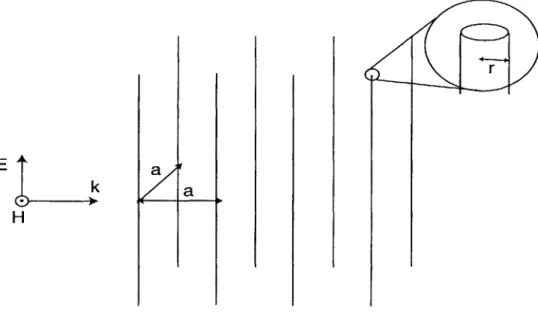
1-1 Array of thin wires in free space leading to negative epsilon
(a = few millimeters and r = few microns) . . . . 20
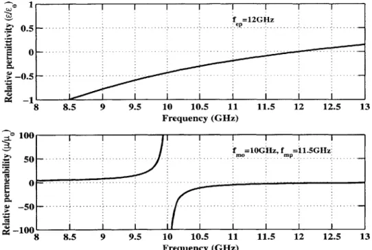
1-2 Typical Permittivity and Permeability functions for LHMs . 21
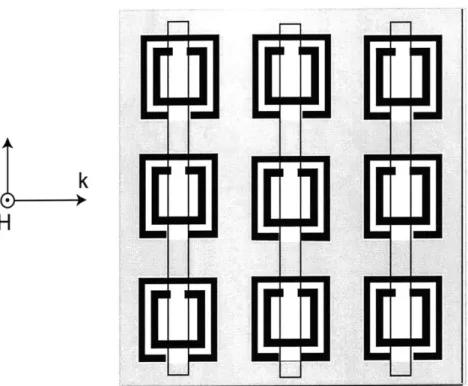
1-3 An array of Split Ring Resonators (SRRs) leading to a nega-tive permeability (Unit cell is of the order of a few millimeters,
ex: 4mm x 4mm) ... ... 21
1-4 A set-up of metallic rods and split rings on a dielectric
sub-strate forming an LHM ... . 22
1-5 A set-up of Omega rings on a dielectric substrate forming an
L H M . . . . . 22
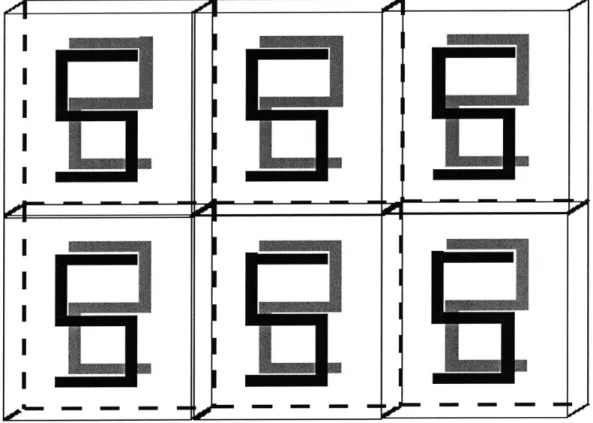
1-6 A set-up of S rings forming an LHM. Each unit cell contains two S shaped rings printed on the two sides of a dielectric
substrate . . . . 23
2-1 The S-shaped SRR (Dimensions (in mm, not to scale) : a= 5.2, b-2.8, c=0.4, h=0.5, dx=4, dy=2.5, dz=5.4) . . . . 27
2-2 Set-up of a unit cell of S-rings inside a rectangular Waveguide 27
2-3 S-parameters for one layer of S-rings with dimensions as shown
in F igure 2-1 . . . . 30
2-4 S-parameters for two layers of S-rings with dimensions as
shown in Figure 2-1 ... 31
2-5 Retrieved Refractive Index for one Layer of S-rings with di-mensions as shown in Figure 2-1 . . . . 32
2-6 Retrieved Refractive Index for two Layers of S-rings with di-mensions as shown in Figure 2-1 . . . . 33
2-7 Surface Current density (J) on the front and back rings of
the S-shaped SRR with dimensions as shown in Figure 2-1 . 34
2-8 Fourier expansion of J on the front ring of the Unit Cell shown in Figure 2-1 . . . . 35
2-9 Fourier expansion of J on the back ring of the Unit Cell shown in Figure 2-1 . . . . 36
2-10 Local and Global Coordinate systems of a Unit Cell . . . . . 39
2-11 A typical array of elements on the x-y plane . . . . 40
2-12 Array Patterns for linear arrays obtained using (2.22). Solid Line: N-2, d=A/2, Progressive phase (a)=O. Dashed Line: N = 2, d= A/2, a=7 . . . . 42
2-13 Array Patterns for a linear arrays obtained using (2.22). Solid
Line: N=3, d=A/2, a=O. Dashed Line: N=2x2, d=A/2, a=O 43
2-14 Array Pattern for a linear arrays obtained using (2.22). Solid
line: N=5, d=A/2, a=7r. Dashed Line: N=5, d=4A/5, a=-r . 44
2-15 Surface current density on the First ring in the propagation direction inside a waveguide . . . . 45
2-16 Surface current density on the Second ring in the propagation direction inside a waveguide . . . . 46
2-17 Surface current density on the Third ring in the propagation direction inside a waveguide . . . . 46
2-18 Phase difference between adjacent rings . . . . 47
2-19 A sam ple prism . . . . 48
2-20 Normalized Radiation due to prism with angle r, = 390 The
2-21 Normalized Radiation due to prism with angle r = 28" The solid slanted line shows the prism edge, and the dashed line
shows the norm al. . . . . 50
3-1 A Uniaxial slab with optic axis along the x-axis . . . . 61
3-2 Schematic diagrams of TE and TM Incidence . . . . 63
3-3 Fresnel coefficients for an isotropic slab (no = n, = 1.5, q = 50') 67 3-4 Fresnel coefficients for free-space(no = ne = 1,
#
= 50') . . . . . 673-5 Fresnel coefficients for non-lossy uniaxial slab(no = 1.5, ne = 2, 450) . . . . 69
3-6 Fresnel coefficients for non-lossy uniaxial slab . . . . 70
3-7 Leakage in 0-type versus E-type polarizers . . . . 72
3-8 Leakage in different types of polarizers . . . . 72
3-9 Fresnel coefficients for an 0-type polarizer(no = 1.5, ne = 1.5 + 0.03i, # = 0) . . . . 74
3-10 Fresnel coefficients for an E-type polarizer(no = 1.5+0.03i, ne = 2.1, = 0) . . . . 75
3-11 Fresnel coefficients for an 0-type Metamaterial polarizer(no = 2, ne = 2i, 0 = 0) . . . . 75
3-12 Fresnel coefficients for an E-type Metamaterial polarizer(no = 2ine= 2,# = 0) . . . . 76
List of Tables
2.1 Limits on the J for different sections of the ring (L=total
Length of the ring, s=L/5, d=dy=0.5mm) . . . . 37
Chapter 1
Introduction
1.1
Historical Background
There has been a recent upsurge of interest in the electrodynamics of media
hav-ing negative permittivities and permeabilities, in selective frequency bands in the microwave regime [1]. These media, popularly known as metamaterials, posses a
neg-ative refractive index (n) in the spectral region where both the permittivity (c) and permeability (p) are negative. Also known as Left-Handed Media (LHM), a wave propagating in one such medium has its phase reversed such that the wave vector, the Electric Field and the Magnetic Field form a Left-Handed (LH) triad. As a con-sequence, the wave vector and the Poynting vector are opposite in direction for an
isotropic LHM. The prospect of realising a negative index of refraction, and the many other interesting phenomena that LHM promise, opens up wide ranging applications
that were hitherto considered impracticalities.
LHM were first studied by Victor G. Vesalago in 1968 [3]. Veselago studied a hypothetical LHM, noting that c and p can be simultaneously negative in a particular frequency band, only if they are dispersive. Given the fact that there was no such
material known at that time, the study in [3] was one of predominantly theoretical interest, albeit a highly imaginative one. Assuming an hypothetical LHM, however, the said work elucidated some of the most important consequences of such media
as reversed Doppler effect, anomalous refraction phenomena, etc, for the first time. The frequency dispersion was proposed to be Drude-type for both c and ft. The existence of plasmas having a Drude-type effective e was known for long. But the justification for the possibility of a magnetic analogue, as presented in [3], had neither a firm theoretical basis nor any experimental verification. The non-existence of such a
media with simultaneously negative E and p, precluded any progress in this direction for about the next 30 years.
However, with the advent of improved fabrication methods and novel artificial
electromagnetic structures like photonic crystals, etc., curiosity about negative e and p revived in the 90's. Negative permittivities were known, for long, for plasmas in solid state [4][5]. Surface plasmons in metals give rise to a Drude-type dielectric function
leading to negative permittivities at frequencies in the optical range. However, at lower frequencies, high losses come into play and the negative 6 effect is nullified.
This fact, along with the difficulty of having magnetic resonances at high frequencies, posed a serious impediment to realising LHMs. One of the first attempts to overcome
this limitation was made by Pendry et.al (1996) [6]. Their work proposed a geometrical scheme in which the plasma frequency of a metallic structure could be obtained in
the Microwave regime. They considered an assembly of thin metallic wires, of the order of 1pm cross-sectional radii, which constrained the plasmons to oscillate along the wires. The plasma frequency in a metal is, in general, a function of the number density and mass of the oscillating electrons. However, by constraining the electrons to the thin metallic wire assembly, their effective number density is greatly reduced
and the effective mass enhanced. This synergism leads to a reduced plasma frequency for the entire structure. The plasma frequency, as shown in [6], is dependent only on the macroscopic geometrical parameters of the structure, namely, the radius of the wires and the lattice spacing of the assembly. Considering a lattice of aluminium wires
of 1pm radius and 5mm spacing, a plasma frequency of 8.2 GHz was obtained in [6] and [7]. Numerical simulations and experimental verification of the results confirmed
was rendered possible. However, the negative p still remained elusive at that point. .
A composite material which could give a desired magnetic response was the goal.
As long as the unit cell of the composite is small compared to the wavelength of the electromagnetic radiation, the composite can be considered to be homogenous. It is
then just a matter of determining the effective permeability of the composite material in terms of the parameters of the unit cell, just as our conventional notion of perme-ability of a material medium is a definition in terms of the properties of the atomic constituents. This was the concept on which Pendry et. al (1999) built upon, culmi-nating at a landmark metallic geometry which promised a negative permeability in
the microwave regime. Starting with an array of thin metallic cylinders, and working through some examples of magnetic microstructures, they finally derived the effective permeability due to a split ring structure [8]. The final structure was a three dimen-sional stack of split ring resonators (SRRs), each unit cell measuring about lsq.cm.
The effective permeability of such a system was derived to be resonant in form. An SRR could be decomposed into a set of capacitative, inductive and resistive elements.
An incident magnetic field induces currents in the circular loops of the rings, thereby forming an RLC circuit. The Inductance, Capacitance, and the Resistance of the cir-cuit were purely a function of the frequency and the geometrical parameters. Thus, with an appropriate choice of the parameters, a resonance frequency in the desired range could be obtained. Proceeding thus, a resonant frequency of 13.5 GHz was
obtained. This marked the onset of artificial electric and magnetic microstructures, combinations of which were capable of obtaining negative c and p in the microwave range, simultaneously.
1.2
Basic Principles
Before delving into deeper ramifications of the LH behavior of these artificial media, it is pertinent to ponder over some of the basic principles guiding this behavior. In as much as the negative refractive index is concerned, all we are concerned about is the possibility of a negative e and a negative p, simulataneously. However, the forms of
the permittivity and permeability functions that have been realised practically, and the conditions that need to be met to obtain the same, form an interesting aspect of this area.
1.2.1
Negative Permittivity
Negative E in conventional LHMs is obtained by an array of thin metallic wires, of specific dimensions [6]. A typical set-up of the rods in free space is shown in Figure 1-1. For a plane wave excitation, with the Electric Field (E) vector along the wires, the free charges in the metal are set to oscillate along them. By keeping the cross-section of the wires very small, the effective density of the charges in the lattice space is greatly reduced and the effective mass enhanced. The plasma frequency is given by,
2 ne2
CoMeff
where, n is the number density of the charges (plasmons) and meff is the effective mass of the charges. Thus, by decreasing the density and increasing the effetive mass, the plasma frequency can be lowered. Theoretical analyses and experimental observations support this phenomenon. [6] [9]. It has also been verified that such a effective medium has an effective permittivity given by:
f2
E = E0( -e P"f (f + 7y/2ir)
where,
fe
= wp/(27) is the plasma frequency and y is inversely proportional tothe conductivity of the medium and has units of frequency. A plot showing E(f), for
y= 0GHz is shown in Figure 1-2.
Apart from wire structures which give a negative effective permittivity, some other structures have recently been proposed and experimentally verified. Two of the most recent ones are the Omega structure [11] and the S structure [12]. All these
struc-Field. Thus, common to all LH structures is the underlying phenomenon that an elec-tric field parallel to thin metallic structures constrains the charges to oscillate along the structures giving rise to a plasma behavior, and hence a plasma-type dielectric
function.
1.2.2
Negative Permeability(p)
Negative [ in LHMs is obtained by an array of metallic split rings, commonly known
as Split Ring Resonators (SRRs). A typical set-up of periodically spaced SRRs is shown in Figure 1-3. Also shown in the figure, is the wave incidence direction leading to a negative permeability. The rings are in the plane of the paper and the Magnetic Field (R) is directed out of the plane of the paper. A varying magnetic field in this direction induces currents in the loops of the rings. The geometry of the rings
leads to effective capacitances and resistances in the path of the current [8]. These capacitative and resistive elements along with the current loop form an RLC circuit. The resonant frequency of this circuit depends purely on the geometry of the metallic
structure, and has been succesfully realized in the microwave regime.
The effective permeability of such a structure is given by,
S= - 1 fo(2f2 )
f2- fmL + i-y/2Ir
where, fmp is the magnetic plasma frequency, fmo is the magnetic resonant
fre-quency and -y is the loss component having units of frefre-quency. A plot showing the resonant behavior of the permeability is also shown in Figure 1-2, with y = 0GHz.
1.2.3
LHM Geometries
As seen in the previous sections, thin wire shaped metallic elements (rods) parallel to the
E
and metallic loops in the plane perpendicular to the H of an incident plane wave give rise to a plasma-type c and a resonant p respectively. The overlapping frequency band, where c and p are simultaneously negative, is the LH band. Thuscombinations of rings and wire elements have been widely used to realize LHMs in the microwave regime [9] [10]. Figure 1-4 shows a typical set-up of a ring-rod combination with the proper incidence which gives rise to LH behavior.
E a
k a
H
Figure 1-1: Array of thin wires in free space leading to negative epsilon (a few millimeters and r = few microns)
Apart from the standard SRR - rod combination, which were traditionally used to obtain LHM, new structures have been introduced in the recent past to achieve the same purpose. Figure 1-5 shows an array of Omega shaped rings forming an LHM. In this case, two omega rings are placed one behind the other and each ring being a mirror image of the other. Figure 1-6 shows an array of S shaped rings forming an LHM. As in the case of the omega rings, here also the two S-rings are placed one behind the other as mirror images.
--1 f=12GHz Frequency (GHz) ... -in~ 50 0 -50 S-100~ .- -. -
.-. .-
-8.5 9 9.5 10 10.5 11 11.5 12 Frequency (GHz) 3 12.5 13Figure 1-2: Typical Permittivity and Permeability functions for LHMs
E
H
k
Figure 1-3: An array of Split Ring Resonators (SRRs) leading to a negative permeability (Unit cell is of the order of a few millimeters, ex: 4mm x 4mm) f =10GHz, f =11.5GHz m- - -...... ... ... .-. ... .-.. ....
Ea
Elm]
Elm]
Ea
Ea
E
k
H
II
Figure 1-4: A set-up of metallic rods and forming an LHMsplit rings on a dielectric substrate
Figure 1-5: A set-up of Omega rings on a dielectric substrate forming an LHM
I I
II II IIK
II
II
II
I!- El !~~LuImE I
-I
I
I
I
I
I
I
I
I
I
-t E-I
I
I
I
I
Figure 1-6: A set-up of S rings forming an LHM. Each unit cell contains two S shaped rings printed on the two sides of a dielectric substrate
_+.OPI_ -
-
-
-LPOI-
-
-
-
Chapter 2
Radiation due to S shaped SRR
2.1
Introduction
Conventional Left-handed materials have been fabricated using composites of metallic rings and rods. The rings, commonly known Split Ring Resonators (SRR) [8], lead to a resonant effective permeability (p). And, the rods, which are thin metallic wires, lead to a plasma type effective permittivity (e) [6]. In the overlapping frequency band, where c and p are both negative, a negative refractive index (n) is observed leading to
the well-known Left-Handed (LH) behavior of the composite material. It was recently demonstrated that S-shaped metallic structures (S-rings) exhibit LH characteristics
equivalent to an SRR-rod combination [2]. And, negative refraction in a prism made of such structures was experimentally verified [12] , in the frequency band roughly between 15GHz-20GHz, depending on the physical dimensions of the setup.
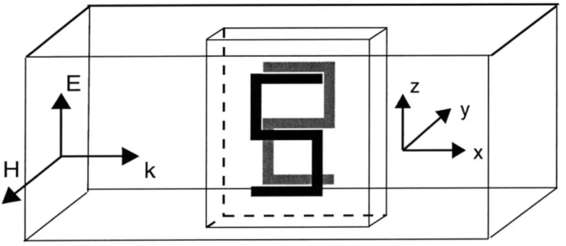
An S shaped SRR consists of two parallel S-rings oriented oppositely as shown in Figure 2-1. A varying magnetic field perpendicular to the parallel plane of the rings
induces currents along the rings. These currents along with the resistive, capacitative and inductive elements imposed by the geometry of the rings, lead to a resonant
mag-netic response similar to that in a conventional SRR. Also, an incident electric field along the longer sides of the rings, in the parallel plane, induces a plasma type electric response similar to that in an array of thin rods (the conventional rod medium).
In this section, the radiation characteristics of composites made up of such
S-shaped SRRs are studied in detail. Numerical simulations using the Ansoft HFSS TM numerical package lead to an understanding of the currents induced due to a plane wave excitation on each of the two S rings in an SRR. The incident plane wave is a
TEM mode at 17GHz, with the Electric Field vector in the plane of the ring and the
magnetic field vector perpendicular to the plane of the ring. The values of the surface current density (J) are obtained at discrete positions along each S-ring. A discrete fourier transform of this data allows one to express J as a fourier expansion. This facilitates an analytic expression for J along a ring as a function of the normalized distance along the ring. The current density thus obtained is used to determine the vector current moment due to the ring [2]. The far field radiation due to the ring is then determined using this vector current moment. The radiation pattern to a single S-ring is found to be symmetric in nature and resembles a radiation pattern due to a combination of dipoles stacked along the segments of the S-ring with the given current distribution.
In order to determine the far field radiation due to a composite made up of S-rings, the array factor specific to the composite structure is determined first. This array factor coupled with the radiation pattern due to a single ring gives the pattern due to the composite. The progressive phase increment between rows of the array are obtained from HFSS TM simulations of a slab of shaped SRRs. Prisms of S-rings with different prism angles and dimensions are studied. It is observed that the characteristic negative refraction of the composite is observed considering the edge elements of the prism, and using a negative progressive phase shift. On the other hand, considering all the prism elements leads to substantial diminution of the distinct lobes and a radiation pattern concentrated parallel to the incidence direction
L C - h~
a
5-. dy 72 z y dxFigure 2-1: The S-shaped SRR (Dimensions (in mm, not to scale) : a= 5.2, b=2.8, c=0.4, h=0.5, dx=4, dy=2.5, dz=5.4)
E
H
zt
Z
y
x
k
I-Figure 2-2: Set-up of a unit cell of S-rings inside a rectangular Waveguide
b dz
Z/000/
I
ZZ
AZZ
I2.2
S-parameters and Effective Refractive Index
The simulation setup of an S shaped SRR inside a rectangular waveguide is shown in Figure 2-2. The boundaries of the waveguide parallel to the rings are assigned to be Perfect Magnetic Conductors (PMC) so as to facilitate a TEM mode as the fundamental mode. The incidence is a plane wave with a frequency of 17GHz, which lies in the resonant band. The dimensions of the unit cell containing the two rings are shown in Figure 2-1. The setup was simulated using HFSS TM .
Two cases were studied corresponding to one and two S-rings placed along the propagation direction in the waveguide. These two cases correspond to increasing thickness of the effective medium made up of the S-rings, and we denote them as one-layer and two-layer respectively; a layer corresponding to one SRR in the wave guide along the propagating direction.
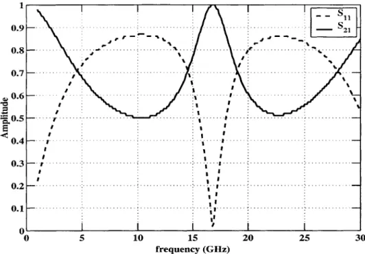
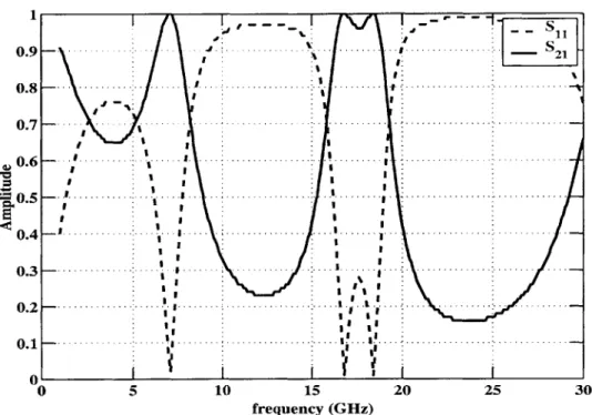
With the set up as mentioned above, the S-parameters, S11 and S21 were obtained for the two cases. As is well-known, the magnitudes of S11 and S21 correspond to the reflection and transmission coefficients of the medium, respectively. Figures 2-3, 2-4 show the S-parameters in the two cases. It can be observed in the figures that there is a band of high transmission around 17 GHz and the transmission falls off rapidly for other frequencies. It can also be seen that as the thickness of the effective slab, i.e the number of layers, is increased the peak band gets slightly wider.
Such a peak in the transmission spectrum for an LH Medium corresponds to the resonant band where the refractive index (n) is negative. For frequencies lying outside this band, only one of c and p are negative. This leads to an imaginary refractive index which causes significant attenuation of the incident wave and hence very low transmission. However, it should be noted that obtaining such a peak in the transmission spectrum does not always imply LH behaviour. The possible LH behaviour can be verified by retrieving the material parameters of the medium, namely n, c and p, from the S-parameters.
for LH media can be found in [18],[19] and [20]. The general approach followed in
these studies was to obtain the n and the impedance, z, of the material medium from the S-parameters and then retrieve the e and p from the n and z, using p = nz and e = n/z. However this approach has been known to be inaccurate in certain cases.
These associated problems were studied in greater detail in [17]. Xudong et. al. have
developed a robust method to overcome the problems of the previous method and to obtain the material parameters from the S parameters in [17]. This approach has been used in the present work to retrieve the material parameters of the medium composed of S-shaped SRRs, from the S-parameters shown in Figures 2-3 and 2-4.
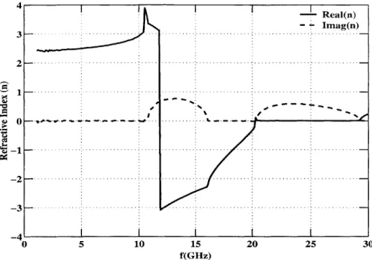
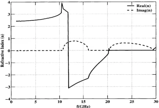
Figures 2-5 and 2-6 show the frequency dependant refractive index (n) for the cases with one and two layers respectively. It can be seen that the refractive index is negative in the frequency band ranging approximately from 12GHz to 20GHz. This
is a confirmation of LH behaviour of the effective media. It can be observed that the figures are nearly identical, confirming the accuracy of the retrieval procedure.
Also, the high transmission regions in the S-parameter plots fall within this band, and peaking at 17GHz (as in Figures 2-3 and 2-4). The refractive index at 17GHz, i.e resonance, as obtained from the retrieval (Figures 2-3 and 2-4) is found to be -1.59.
This is the effective Refractive Index (n) of the S-ring medium at resonance.
In what follows, the surface current densities on the S-rings in the wave guide
setup are studied. These currents are then used to determine the radiation pattern of an S-ring prism. The angle of refraction obtained with such a prism is used to
determine the effective n of the S-ring medium. The n thus obtained is compared with the n obtained in the present section.
2.3
Current Modes
Solving the setup as shown in Figure 2-2, with HFSS TM, with the appropriate mesh
refinement and other numerical parameters, allowed the computation of J for each ring along a trace running along the centerline of the ring. A plot of J thus obtained
1 S .. .... 9. . .. . . . - - - . . . ... - - -. . . .....2 .-. - - 0.8-0.7 Ii e 0.6 . - - -I1 0.4 --,% 0 .. . . ... . . .. .. ..% .I. .. .. .. . . . . .. .. . . 0 . .. . . . ... .. . .. . .. . . .. .. . .. . . . .. . .. . . . .. . . 0.3 - -a 0 7& . .... 0.5 25 30 frequency (GHz)
Figure 2-3: S-parameters for one layer of S-rings with dimensions as shown in Figure 2-1
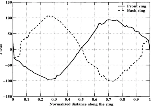
is shown in Figure 2-7.
The plots of J for the two rings suggest that J is a periodic function of the normalized distance along the ring
(1)
i.e. J =J(l), with boundary conditionsJ(O) = J(1) = 0. Assuming J(l) is a continuous function, one can try to expand
J in terms of its Fourier components as:
J(l) = a0 + Z(ansin(2irnl) + b7cos(2wrnl)) (2.1) 7=1 where, a0
10
dlJ(l) a72 = 2jdl
J(l)sin(2zrrl)f.dlJ(1)cos(2nl)
1 - - --0.7- -- 1 0.9 - - -0 .7 . - * - --.-..-..--.. 0 *=0.7 0 . .. . .I. . . . 0.6 . .... I% ~0.2 ... 0.3 0 0 5 10 15 20 25 30 frequency (GHz)
Figure 2-4: S-parameters for two layers of S-rings with dimensions as shown in Figure 2-1
In the present case, however, we have a discrete set of data for each ring. The
Fourier components for this situation can be obtained using the Fast Fourier Trans-form method. A MATLAB function was used to implement this. Figure 2-8 shows a
plot of the actual J along with 21 Fourier components, for the front ring. Figure 2-9 shows the corresponding plot for the back ring.
As can be seen from the plots, in each case there is one dominant mode
cor-responding to n=1 in the expansions. Thus the total J on each of the rings can be approximately represented using a single dominant mode, although the next few
significant modes could also be included in the representation. Thus we have an analytical expression for the currents along the rings. This facilitates the analytical derivation of the radiation fields due to the pair of rings, as in the following section.
4 3 2 o --2 -3 -4 I I Real(n) - -- Imag(n) -.. ..... - .-.. -.. .-. . . -.. . -. -.. . --... ... 0 5 10 - - -. -. -. -.. ..-.. . . .. . . . .. . .-.. . . .-.. 15 f(GHz) 20 25 30
Figure 2-5: Retrieved Refractive Index for one Layer of S-rings with dimen-sions as shown in Figure 2-1
2.4
Radiation due to S shaped SRR
The set-up of an S-ring geometry is shown in Figure 2-1. Each ring is in the x-z plane
with the longer side of the ring along the z-axis and the shorter side along the x-axis. The ring can be viewed as five distinct rectangular metallic elements each of which is
either along the x-axis or along the z-axis. As mentioned in (2.1), the current density along the ring can be expressed as a sum of the fourier modes. We can thus express the current density along each ring as:
N 2n7rs
J(s) = E assn( L
n=1
(2.2)
where, N is the number of significant modes, s is the length along the ring and L is the total length.
4 3 2 1 0 U Cu -. .- -.-. -2 -3 . .. ... . 0 5 10 15 f(GHz) 20 25 30
Figure 2-6: Retrieved Refractive Index for two Layers of S-rings with di-mensions as shown in Figure 2-1
2 n7r
Jx = 2 ansin( L (b + x))6(y - y1)6(z - zi)
n=1
2 nir
Az
= i>
ansin( Lf(b + z))6(y - y1)6(x - Xi) (2.3)where, 6(y) is the Dirac Delta funtion and b is a real scalar quantity determined
by the positions of end points of the segment under consideration.
In order to determine the radiation due to a current carrying element, it is con-venient to first determine the vector current moment [1] given by:
f(0, #) = d' f(?')e- ' (2.4)
For the present problem, we need to determine the vector current moment (f) for the current distribution given by (2.3). Let us consider a typical current distribution of the form: I I ReaI(n) - Imag(n) . ... .. ... . . . . . . . . . . ,a' -.-.- --.. . . . .- . . .. . .-. -. ...- -. ...- ...-. I Real n) - -- -. . .. .--. ..
I I I Front ring Back ring 150 100 -150' 0 I 0.1 0.2 0.3 0.4 0.5 0.6 0.7 0.8 0.9 1
Normalized distance along the ring
Figure 2-7: Surface Current density (J) on the front and back rings of the S-shaped SRR with dimensions as shown in Figure 2-1
n7r (
Jxn = ansin(- (b + x')
L )6(y' - y1)(z' - z1
)
(2.5) where, x' E [xl, x2], i.e the segment of the ring is along the x-axis.The f, denoted as fx for this case, can be determined as,
=x x dx'dy'd z'ansi 2nj (b+ x'))6(y' - y1i)6(z' - z1)e-i(kxx'+kvy'+kzz')
= iane-i(kyy1+k z1) e- i(kyy1+kzi) X2 nr x' dx' siri(-L(b + xI))e-Icxx" )) c ( fxn =xan (2.6) . ..... .. .... ... ... ... ... .... .. ... .. ... ..-- ..---. -. .. ... .-. ---. . .. .. . . .. .-. - -. . . .. .-. -.- -. .... .-- - -- - - - -- -% -- . . . ... . . .--. . .. . .- .. .- .. . . .--.. .--.. --.. .. -. . . -.. . --. -. . . . .. . . .-. -. -. . . . . . . . . .. . .-.-. . -. -50 'U 0 0 -50 -100
100 ' 7 L -- TotalJ O 80 - Fourier modes 4 0 - ..-...--..-...--.. 0 -100 0 0.1 0.2 0.3 0.4 0.5 0.6 0.7 0.8 0.9 1 Normalized distance along the ring
Figure 2-8: Fourier expansion of J on the front ring of the Unit Cell shown in Figure 2-1
Thus the total vector current moment including all the fourier modes under
con-sideration, can be expressed as:
N e-i(kyy1+kzzl)
= an n2a2 - k2 [ikxsin(na(b + x')) + nacos(na(b
+
x ))e-ikX1 (2.7)where, [g(x)]X = g(x2) - g(xl).
Similarly proceeding for the case when the segment is along the z-axis, we have:
2 ei(kyyl+kxx1)
fz = an n2 2 - k2 [ikzsin(na(b + z')) + nacos(na(b + z'))e-zz1Z (2.8)
n=1 Z
Equations (2.7) and (2.8) give the general forms for the vector current moments
along each segment of the ring, depending on whether the segment is along the x-axis or the z-axis. Thus for each segment the
f
vector can be obtained using the known-- Total J - Fourier modes
-00 0.1 0.2 0.3 0.4 0.5 0.6 0.7 0.8 0.9 1 Normalized distance along the ring
Figure 2-9: Fourier expansion of J on the back ring of the Unit Cell shown in Figure 2-1
values of the independent variables, b, yi and
[xi,
x2] (or[zi,
z2]).
The S ring has five such segments. The total
f
of a single S ring, due to all the segments, is the vector sum of those due to each of the individual segments.5
Iring
= f p (2.9)p=1
The S-shaped SRR is composed of two S rings as shown in Figure 2-1. Thus, the total
f
vector due to both the rings can be obtained as:5
p=1
where, the superscripts 1 and 2 refer to the two rings.
The various values of the independent variables b, Yi and
[xi,
x
21
(or
[zi,
z2])
corresponding to the different segments of the two rings are tabulated in Table 2.1.
Front Ring Back Ring f b X Y 1 z f b c1 Y1 zi x 0 [0,s] 0 0 -x -L [s,0] d 0 z s s 0 [0,s] -z s-L 0 d [0,s] -x -3s [0,s] 0 s -x 2s-L [0,s] d s z 3s 0 0 [s,2s] -z 3s-L s d [s,2s] x 4s [0,s] 0 2s x -5s+L [s,0] d 2s
Table 2.1: Limits on the J for different sections of the ring (L=total Length of the ring, s=L/5, d=dy=0.5mm)
Sfx + fz. The components
fo
andfo
can be obtained by making a cartesian to spherical transformation.By noting the transformation,
J = f sin(O)cos(O) + 9cos(O)cos(O) - qsir(#)
= fcos(6) - Osin(6 ) we have,
fo
= cos(6)cos(O)fx - sin(O)fz fo = -sin(#)fx (2.11) (2.12)where, 0 and
#
are the conventional polar angles in the spherical coordinate sys-tem.Thus we can obtain the far-field radiation for the S-shaped SRR. The radiation
pattern can be determined using
[21:
ikr
E(f) = iwpu (Ofo + Ofo) 47rr
eikr
H(F) = eikr(fo - Ofo) (2.13)
47r
<(>= )2( f~j2 + If4|2)
2 47rr
2.5
Array Pattern Formulation
2.5.1
Vector Current moment for an arbitrary unit cell
A unit cell (refered to as an 'element' henceforth) consisting of a pair of S-rings and a substrate is shown in Figure 2-1. The local co-ordinate system(LCS) of the unit cell is shown in Figure 2-10 with primed vectors. The surface current density
(J)
on the rings, as developed in the previous sections, can be expressed in terms of the local position coordinates. Let us consider an element with local origin at a position
Po(xo, yo, zo) in the global coordinate system (GCS). Let the position PO be denoted by the position vector, fo, in the GCS. We denote any arbitrary point (P) in the source region (i.e. in the element) by the position vector i' in the GCS. Then, the
position vector of the point P in the LCS is given by Fo = f' - fo, as shown in Fig.3.
Therefore, J= J(V') = j(fs) = J(' - fo)
The vector current moment due to an element at P is given by:
fo =
ffJ
di'(')e~ff1
d'J(fo')e--' (2.14)Noting that fi f' - Fo, we have:
o = e-kdffo J d I(fo-o)e-o' (2.15) Analogous to the above case, we can also consider another element at a point P1
given by the position vector fi in the GCS. Then the position vector of an arbitrary point P in the LCS is given by f'i = ' - fi. Then, proceding similarily as above, the
-
P
0
_,Figure 2-10: Local and Global Coordinate systems of a Unit Cell
fi = ea'r1
fJ'
JJ(fi')e-
I'
(2.16)By making a change of variables and noting that the local geometry of all unit
cells are indentical, we have:
fi =e '
Jig1
dfO J(fo')e-i0' -eik-(fo) fo (2.17)Thus for any arbitrary unit cell at a point Pa, the
f
vector can be expressed in terms of that of a unit cell at a global reference point Po, as:fi = e-a ik( o) fo (2.18)
Az
Z'y
: I -mm* X'
D2.5.2
Array Factor
Let us consider a group of elements as shown in Figure 2-11 with unit cell dimensions
dX, dy and d, in the x,y and z directions respectively as already mentioned in Figure
2-1. The array factor due to an element with position indices [m,n,q] along [x,y,z] can
be expressed using (2.18)as:
y
Umno
q z !r p xFigure 2-11: A typical array of elements on the x-y plane
(2.19)
fmnq = e -ik'mnq+iamnqfo
where, fo is the
f
vector of the unit cell at the origin, and amnq is a progressive phase shift.As an example, for a cubical array pattern with M, N and
Q
number of unit cells in the x,y and z directions respectively, the f due to all the elements is given as:(2.20)
M-1 N-i Q-1
f
f=
f
0 E ES
e~-ik(msin()cos(+)+ndvsin(O)sin(+)+qzcos(0))+iamnq (2.21)m=O n=O q=O
Therefore,
M-1 N-1 Q-1
F =
E S
E e -ik(m(si2(2)2os())+ndysin(O)sin(o)+qdcos(O))+iamnq(.2
m=O n=O q=O
is the array factor for the said cubical array pattern.
Thus, the array factor for any type of pattern can be obtain from (2.22) by defining the appropriate limits on [M,N,Q] and the corresponding summation scheme.
2.5.3
Validation
The Array factor formulation as determined above is validated here for known cases of antenna arrays. For all the cases presented here, all the array elements are on the
x-y plane. And,the magnitude of the array factor, F, is plotted on the x-y plane, i.e 0 = 7r/2, as a function of the angle 0. Figure 2-12 shows the plot for a two element
array (M=2,N=1,Q=1) along the x-axis with an inter-element distance (d. = dy =
d = A/2), and varying values of the progressive phase (a). Figure 2-13 shows the plot for a three element array (M=3,N=1,Q=1) along the x-axis with d= A/2, and a = 0, and that for a 2 x 2 element array (M=2,N=2,Q=l) on the x-y plane. And, Figure
2-14 shows the plots for N=5, a = 7r and d= A/2 and d= 4A/5.
All these plots conform to those obtained using known analytical methods for
determining array factors for antenna arrays [2]. Thus the formulation developed here can be treated as general and can be applied to any geometry by appropriate selection of the variables.
90 2 120 60 150" - 30 180 -. .. . -.. -..- 0 210 330 240 300 270
Figure 2-12: Array Patterns for linear arrays obtained using (2.22). Solid Line: N=2, d=A/2, Progressive phase (a)=0. Dashed Line: N=2, d=A/2,
a=7r
2.6
Results
2.6.1
Determining the progressive phase
Inorder to determine the radiation pattern due to an S shaped SRR element, one needs to know the amplitude and phase of the current density each ring of the SRR. As seen in the previous sections, the current density on each ring can be expressed interms of the fourier modes and an anlytical expression can be thus be obtained.
Using these current modes, the radiation pattern for each SRR can be obtained. We have also developed a general formulation to obtain the array factor due to a
composite made of such SRR elements. Using the radiation pattern due to a single ring and the array factor due to a composite structure, the radiation pattern due to
the total structure can be determined. It is pertinent at this point to consider the inputs that are required to obtain this total radiation pattern. As is clear from the formulation, the only inputs that are required, other than the current distribution
90 3 120 6 150 -30 180 ---.- -..--.-- 0 210 330 240 300 270
Figure 2-13: Array Patterns for a linear arrays obtained using (2.22). Solid Line: N=3, d=A/2, a=0. Dashed Line: N=2x2, d=A/2, a=O
elements, and (2) the progressive phase change between subsequent elements.
Inorder to determine these parameters, we study the case of an infinite slab con-sisting of such elements, simulated using HFSS TM. The set-up is similar to that of
Figure (2-2), except that we now have three elements in the direction of propagation as opposed to one element in Figure (2-2). Having three elements facilitates us to
study the amplitude and phase of the currents on each of the three SRRs in the di-rection of propagation. The infinite dimensions in the other didi-rections are achieved
using the PEC/PMC boundary conditions as shown in Figure (2-2).
Figures 2-15 to 2-17 show the amplitudes and phases of the surface current den-sities (J) on the front rings of each of the three SRRs, along with the total J. Each
Figure has four plots showing (a) Magnitude of each component of J (Jx,Jz Mag)
(b) Phase of each component of J (Jx,Jz Phase) (c) Total value of each component of J (Jx,Jz total), and (d) The resultant J obtained from the two components (J
to-tal), with respect to the normalized distance along the ring. In the last plot showing (J total), the actual values have kinks at the positions corresponding to the corners of the rings due to numerical problems in evaluating the currents at those points.
90 5 120 60 150 2530 1 8 0 ..--- -.. -. .. ... .... ..- ... ...- .. 0 210 330 240 300 270
Figure 2-14: Array Pattern for a linear arrays obtained using (2.22). Solid line: N=5, d=A/2, a=7r. Dashed Line: N=5, d=4A/5, a=r
These kinks have been smoothened using linear interpolation. The interpolated plot is shown along with the actual values. It is to be noted that each ring lies in the x-z plane, so that J has only x and z components.
It can be seen from (2-15) to (2-17) that the amplitudes of each component of (Jx,Jz Mag) are the same for each of the three rings. However, the phase of each component varies across the rings, causing a net variation in the total J. So, for an array of SRR elements along the propagation direction, the amplitude of J along each
of the elements can be expected to be a constant function of the position, however there is a phase difference across the elements. It is thus imperative to examine the
progressive phase increment/decrement between subsequent SRR elements.
Figure (2-18) shows the phase differences between adjacent elements of the three element setup. The figure consists of two parts showing (a) the phase difference between rings 1 and 2, 621 and (b) the phase difference between rings 2 and 3, 632,
as a funtion of the position along the rings. The plots show the phase differences between each component of J, i.e J and J,. However, it is to be noted here that
-200 J 0 0.1 0.2 0.3 0.4 0.5 0.6 0.7 0.8 0.9 1 200 1 1 1 1 x 4 - - JA -200-0 0.1 0.2 0.3 0.4 0.5 0.6 0.7 0.8 0.9 1 a100 .. i 0 -0 0.1 0.2 0.3 0.4 0.5 0.6 0.7 0.8 0.9 1 100 0 -0 actual -1- interpolated -100 02-0 0.1 0.2 0.3 0.4 0.5 0.6 0.7 0.8 0.9 1 Normalized distance along the ring
Figure 2-15: Surface current density on the First ring in the propagation direction inside a waveguide
relevant which has a dominant amplitude. Correspondingly, the value J21 and J32
show the relevant phase differences in each situation. It can be seen from both the
plots that the phase differences between the first and the second rings is same as that between the second and third rings, at every position along the rings, and equals 125'. Using the e'(wt-) notation adopted in HFSS TM in speciying the phase of an
Electromagnetic wave, this difference corresponds to a progressive phase increment
of -125', i.e a = -125'.
This backward increment of progressive phase is one of the indications of an LH
medium. Having obtained a, we can now use it in the array pattern formulation of a required composite struture, and determine the corresponding array factor. This
array factor, in conjuction with the radiation pattern due to a single element will give us the radiation pattern due to the entire structure.
200 1 1 1 1 1 1 1j ~ ~ ~~ ~ Jz 0 -200 0 0.1 0.2 0.3 0.4 0.5 0.6 0.7 0.8 0.9 1 200 -S 0- -.. -. --200' I I I I I I I I 0 0.1 0.2 0.3 0.4 0.5 0.6 0.7 0.8 0.9 1 100 -x -JZ. -100, 0 0.1 0.2 0.3 0.4 0.5 0.6 0.7 0.8 0.9 1 100 00 actual ,--- interpolated _ -100, 0 0.1 0.2 0.3 0.4 0.5 0.6 0.7 0.8 0.9 1
Normalized distance along the ring
Figure 2-16: Surface current density on the Second ring in the propagation direction inside a waveguide
u200 -- jx -Jz 0 -200' 0 0.1 0.2 0.3 0.4 0.5 0.6 0.7 0.8 0.9 1 200 -0E -Jx -200 -T Jz 0 0.1 0.2 0.3 0.4 0.5 0.6 0.7 0.8 0.9 1 100 j C -100 0 0.1 0.2 0.3 0.4 0.5 0.6 0.7 0.8 0.9 1 100 F- -T ctu al e ---- interpolated --100, 0 0.1 0.2 0.3 0.4 0.5 0.6 0.7 0.8 0.9 1
Normalized distance along the ring
Figure 2-17: Surface current density on the Third ring in the propagation direction inside a waveguide
400 1Jz 21 200 - - - 32 Ik I - - - -32 0 0 . ... ... . . . .. . . . Iis .... . ... ... . . ... soi I, Ia L 01 0 0.1 0.2 0.3 0.4 0.5 0.6 0.7 0.8 0.9 1 400 - ~ : : 32 ' 300 - --. .. . -. . -..-.. .-20
0
0.1 0.2 0.3 0.4 0.5 0.6 0.7 0.8 0.9 1Normalized Distance along the rings
Figure 2-18: Phase difference between adjacent rings
2.6.2
Radiation Pattern for S-ring Prism
As seen in the previous sections, the vector current moment for a single SRR can be obtained using (2.11) and the corresponding radiation pattern can be obtained using
(2.13). For an array of elements, the array factor can be obtained using (2.22). The total vector current moment for the array of elements can then be obtained using
f = foF
where,
fo
is the vector current moment due to a single SRR and F is the array pattern of the array of elements.The current formulation will now be used to determine the refracted radiation due
to a prism of S-shaped SRRs. Figure 2-19 shows a typical set-up of the problem. A two-dimensional array of elements forming a prism on the x-y plane is shown. All
the SRRs stand parallel to the x-z plane. The excitation is due to a plane wave propagating in the x-direction, with the
E
vector in the z direction and the H vectorin the y direction. The unit cell dimensions are kept the same, i.e, 4mm, 2.5mm and 5.4mm in the x,y and z directions.
y
E k
0
Figure 2-19: A sample prism
Two cases with prism angles (q) of 28' and 390 are considered. For the y =
28' case, there are 5 elements along the xaxis and 15 elements along the y axis,
forming a 1:3 stagger
(7
= tan-'( 4 = 28.070)). For the 7 = 390 case, there are5 elements along the xaxis and 10 elements along the y axis, forming a 1:2 stagger
=tan--(4 = 38.70)).
A progressive phase (a) of -1250 is used, as determined from the previous section, between adjacent layers of elements along the x axis. And, only the edge elements of the prism are considered to be radiating. These elements are marked in the Figure
2-19. This choice of considering only the end elements is due to the fact that the radiation due to the previous elements is shielded by the successive ones leading to
study about this approach to obtain the radiation pattern is studied in [21]
The results from the two aforementioned cases are shown in Figures (2-20) and
(2-21). As can be clearly observed both the figures indicate maximum radiation on
that side of the normal which pertains to negative refraction. The normals in both the figures are indicated by the dotted lines and the prism-air slanted interface is indicated by a slanted solid line. It can be observed that the angle of refraction (Or)
for y = 28" is 470, in the negative region. Using the Snell's law,
nprismsin(O) = nair Sin(Or)
where, nprism is the effective refractive index of the SRR medium and npi, is the refractive index of free space, we have, nprism = -1.55.
And, for the case with = 390, it can be observed that Or = 660, giving an effective
refractive index of -1.45.
Thus, it can be seen that values of n obtained for both the cases described above approximately match with the n retrieved from the S-parameters (i.e n = -1.59). The apparently minor differences between the values can be attributed to the irregular edges of the prisms.
Prism angle (T)= 39 90 1 120 2 150 0.5 30 1 8 0 ...- . -... . -. -.-.--- . ... . .. .- . 0 210 -. 330 240 300 270
Figure 2-20: Normalized Radiation due to prism with angle = 390 The
solid slanted line shows the prism edge, and the dashed line shows the normal Prism angle (Tl)= 28 90 0.6 120 60 0. 150 -- 30 50 180 ---...-.-.- -.-.-. 0 210 330 240 300 270
Figure 2-21: Normalized Radiation due to prism with angle q 28" The
solid slanted line shows the prism edge, and the dashed line shows the normal