Rating Airborne Sound Insulation in Terms of the Annoyance and Loudness of Transmitted Speech and Music Sounds

Publisher’s version / Version de l'éditeur:

Vous avez des questions? Nous pouvons vous aider. Pour communiquer directement avec un auteur, consultez la

première page de la revue dans laquelle son article a été publié afin de trouver ses coordonnées. Si vous n’arrivez

Questions? Contact the NRC Publications Archive team at

PublicationsArchive-ArchivesPublications@nrc-cnrc.gc.ca. If you wish to email the authors directly, please see the first page of the publication for their contact information.

https://publications-cnrc.canada.ca/fra/droits

L’accès à ce site Web et l’utilisation de son contenu sont assujettis aux conditions présentées dans le site LISEZ CES CONDITIONS ATTENTIVEMENT AVANT D’UTILISER CE SITE WEB.

Research Report (National Research Council of Canada. Institute for Research in

Construction), 2008-11-01

READ THESE TERMS AND CONDITIONS CAREFULLY BEFORE USING THIS WEBSITE. https://nrc-publications.canada.ca/eng/copyright

NRC Publications Archive Record / Notice des Archives des publications du CNRC :

https://nrc-publications.canada.ca/eng/view/object/?id=94f5e424-e5f7-4915-8c7a-499d0530560a https://publications-cnrc.canada.ca/fra/voir/objet/?id=94f5e424-e5f7-4915-8c7a-499d0530560a

NRC Publications Archive

Archives des publications du CNRC

For the publisher’s version, please access the DOI link below./ Pour consulter la version de l’éditeur, utilisez le lien DOI ci-dessous.

https://doi.org/10.4224/20377190

Access and use of this website and the material on it are subject to the Terms and Conditions set forth at

Rating Airborne Sound Insulation in Terms of the Annoyance and

Loudness of Transmitted Speech and Music Sounds

http://irc.nrc-cnrc.gc.ca

Rating Airborne Sound Insulation in Terms of the Annoyance

and Loudness of Transmitted Speech and Music Sounds

D B R - R R - 2 4 2

P a r k , H . K . ; B r a d l e y , J . S . ; G o v e r , B . N .

N o v e m b e r 2 0 0 8

Rating Airborne Sound Insulation in Terms

of the Annoyance and Loudness

of Transmitted Speech and Music Sounds

Hyeon Ku Park, John S. Bradley and Bradford N. Gover

IRC Research Report, IRC RR-242

November, 2008

RR-242 - 1

ABSTRACT

This report describes the results of evaluations of airborne sound insulation measures in

terms of the annoyance and loudness of transmitted speech and music sounds. Subjects

rated sounds simulating transmission through 20 different walls with a wide range of

sound transmission characteristics. The evaluated measures included the standard Sound

Transmission Class (STC) and the Weighted Sound Reduction Index (R

) as well as

variations of these measures. In addition, many other signal-to-noise type measures and

loudness-related measures were included in the evaluations. The results showed that the

frequencies important for rating speech sounds were quite different to those required for

music sounds. As a consequence, measures that predicted ratings of transmitted music

sounds well tended to be less successful for speech sounds and vice versa. Some

compromise measures were found and new spectrum adaptation terms added to R

values

were seen to be a successful and practical means of more accurately rating airborne sound

insulation.

RR-242 - 2

Table of Contents

Page

Abstract 1 Contents 2 Acknowledgements 3 1. Introduction 4 2. Experimental Details 5 2.1 Test facility 5

2.2 Speech, music and noise signals 6

2.3 Simulated Transmission Loss characteristics 7

2.4 Procedure for annoyance and loudness ratings 9

2.5 Subjects 10

2.6 Data analysis procedures 11

3. Evaluation of Standard Ratings Rw and STC 12

3.1 Annoyance versus STC for music and speech 12

3.2 Annoyance versus Rw for music and speech 13

3.3 Loudness versus STC and Rw for music and speech 14

3.4 Comparison of annoyance and loudness ratings 15

4. Effects of Included Frequencies for Arithmetic Average TL Measures 17

4.1 More important frequencies for TL data 17

4.2 Included frequencies for Arithmetic Average of TL values 18

4.3 Comparisons of some better Arithmetic Average TL measures 22

4.4 Effects of included frequencies for Energy Average TL measures 27

5. Variations of STC Ratings 29

5.1 Variations of the 8 dB Rule 29

5.2 Variations of the Total Allowed Deviation 31

6. Variations of RwMeasures 34

6.1 Evaluation of standard Spectrum Adaptation Terms 34

6.2 Evaluation of variations of Spectrum Adaptation Terms 36

6.3 Variations of included frequencies 41

7. Evaluation of Speech Intelligibility Related Measures, Loudness Ratings and related Measures 45

8. Audibility of Transmitted Sounds 56

9. A-weighted Level Differences for Rating Sound Insulation 64

10. Discussion, Recommendations and Conclusions 69

Appendix I. Annoyance Ratings Including Presentation of a Reference Sound. 73

Appendix II. Effects of Language on Annoyance ratings of Transmitted Speech Sounds 79

RR-242 - 3

Acknowledgements

The authors would like to acknowledge that a Korea Research Foundation Grant, funded by the Korean Government (MOEHRD) (KRF-2006-352-D00200) to Dr. Hyeon Ku Park, supported his contribution to this work.

RR-242 - 4

1. Introduction

Airborne sound transmission through partitions separating dwellings and other spaces is

measured over a range of frequencies in standardized tests. In North America the ASTM E90 [1] procedure is used in the laboratory and the ASTM E336 [2] procedure is used in field situations. In most other countries the ISO 140 procedures [3] are usually followed to measure airborne sound transmission through walls and floors. These two approaches are very similar and include single number ratings to reduce the results at a number of frequencies to a single numerical value.

The STC (Sound Transmission Class) from the ASTM E413 standard [4] and the Rw (Weighted

Sound Reduction Index) from the ISO 717-1 standard [5] are quite similar in their derivation and

are widely used to specify the required sound insulation in various situations such as between homes.

The results of previous research [6,7] showed that the ISO Weighted Sound Reduction Index (Rw)

and ASTM Sound Transmission Class (STC) ratings were not good predictors of the

intelligibility of transmitted speech sounds. Although the total allowed deficiency of 32 dB in the

STC and Rw measures was found to be acceptable, the maximum allowed deficiency of the 8 dB

rule was not helpful for predicting the intelligibility of transmitted speech. However, measures that are related to the intelligibility of speech, such as the Articulation Index (AI) [8], the Speech

Intelligibility Index (SII) [9], and the Articulation Class (AC) [10], were more strongly related

with the mean intelligibility scores.

When other types of possible sound insulation ratings were considered, those that were based on arithmetic averaging of decibel values over frequency were more successful predictors of

responses than those based on energy averages over various frequency bands. This was expected, because the well-established AI measure is based on the same concept of a frequency-weighted summation of the signal-to-noise ratios in decibels over frequencies important for the

intelligibility of speech.

Measures that limit the included frequency bands or weight their importance according to their influence on the intelligibility of speech were also seen to be better predictors of the intelligibility of the transmitted speech. Two more successful approaches included an arithmetic average of transmission loss (TL) values over speech frequencies and a new speech spectrum adaptation

term for the ISO Rw procedure.

It is well known that many types of sounds such as music, speech, television/radio, vacuum cleaners etc. can be disturbing to neighbours [11]. Because the initial study only rated sound insulat6ion in terms of the intelligibility of speech, further studies were needed to consider other ratings of airborne sound insulation and other types of sounds.

The present study responded to this need and compared sound insulation ratings in terms of how well they predicted subjective ratings of the annoyance and loudness of transmitted music and speech sounds. As in the previous work, standard sound insulation ratings were evaluated as well as various other possible measures including those found successful in the first study [6].

RR-242 - 5

2. Experimental Details

2.1 Test facility

All tests were conducted in the Room Acoustics Test Space in Building M-59 at the National Research Council in Ottawa. This is a room measuring 9.2 m long by 4.7 m wide by 3.6 m high. It is constructed from concrete and is resting on springs to make it well sound-isolated from unwanted sounds. For the present study, the interior walls of the room were lined with 10 cm-thick absorbing foam, which was covered by curtains. There was a conventional T-bar ceiling with 25 mm-thick glass fibre ceiling tiles installed, and the floor was covered with thin carpet. This interior treatment yielded a quite ‘dead’ space, enabling the experimenters to completely control the sounds within the room. The background noise level in the room was about 12 dBA (measured with the sound simulation system turned off).

The test speech and music sounds were played over loudspeakers positioned at the front of the room located 2m in front of the subject. The background noise was played over another set of loudspeakers positioned above the ceiling, directly above the subject. Figure 1 shows a diagram of the setup. Listener Ambient noise loudspeakers Ceiling Curtain

Transmitted speech and music loudspeakers

Foam

Figure 1. Schematic of cross-section through Room Acoustics Test Space showing the location of the listener and the loudspeakers used to generate the test sound fields.

A block diagram of the electro-acoustic system used to produce the test sounds is shown in Figure 2. The two blocks labelled ‘DME32’ are Yamaha Digital Mixing Engines, which are highly flexible signal processing boxes, able to perform the functions of many interconnected devices such as equalizers, filters, oscillators, etc. The outputs of the DME32s run via the power

amplifiers into high-quality loudspeaker systems (Paradigm Compact Monitors and Paradigm PW sub-woofers). One component in each DME32 was initially configured to equalize the playback path through the power amplifiers and loudspeakers to be flat at the position of the listener’s head (± 1 dB from 60 to 12000 Hz).

The background noises for the test sound fields were generated by a component of one of the DME32 units that can generate broadband noise. This same unit shaped the spectrum and adjusted the level as desired. One channel of the noise output was delayed by 300 ms relative to the other to avoid the two noise signals arriving coherently at the listener’s position. This avoided any unnatural perceptual effects when the listener moved their head.

The speech and music sounds were generated from playback of recorded source material stored on the computer in 16-bit, 44.1 kHz wav-file format. The output of the sound card ran into the second DME32, which performed the necessary equalization and level adjustment. The required

RR-242 - 6

equalizations to simulate the transmission loss of each of the 20 walls were stored in separate ‘scenes’, which can be selected from the computer over the MIDI interface.

Ambient Noise Transmitted Speech

sub-woofer sub-woofer

power amplifiers

DME32 MIDI DME32

MIDI

optical digital audio link

RS232 RS232

Figure 2. Block diagram of the computer controlled electro-acoustic system used to create the test sounds.

2.2 Speech, music and noise signals

The speech test materials were the Havard sentences [12]. Three different sentences were played through each simulated wall. Three music samples were used which were selected from a large number of pieces as being potentially annoying and different styles of music. They were: Rap music (The Roots, “I Remain Calm”), House music (Dizzee Rascal , “Stand Up Tall”) and Pop music, (Cyndi Lauper, “She Bop”). The average spectra of the speech and music sounds, before modification to simulate transmission through various walls, are shown in Figure 3. The music had relatively more energy at lower frequencies, while the energy of speech was strongest in mid-frequencies (100 Hz to 1 kHz).

In the first test in which the subjects rated the annoyance of the sounds, the average SPL of the sound sources were 83.0 dB (72.1 dBA) for the music and 80.9 dB (75.2 dBA) for the speech. The source levels were fixed at levels such that the transmitted sounds varied from barely audible to quite loud for the range of simulated walls.

63 125 250 500 1k 2k 4k 8k 10 20 30 40 50 60 70 80 SPL, dB Frequency, Hz Music Speech Noise

Figure 3. Average spectra of speech and noise source signals before transmission through the walls as well as the spectrum of the simulated ambient noise.

RR-242 - 7

The source sound levels for the second test, in which subjects rated the loudness of the sounds, were reduced by 6 dB relative to those for the annoyance test to make it possible to also determine the threshold of audibility of the transmitted sounds. Figure 3 also includes the spectrum of the simulated ambient noise at the listener’s position, which was held constant at an overall level of 34.7 dBA.

2.3 Simulated Transmission Loss characteristics

The 20 simulated wall transmission loss characteristics were the same as in the previous speech intelligibility experiment [6]. They simulated real walls with a wide range of STC ratings evenly distributed between STC 34 and STC 58 as obtained in standard laboratory sound transmission loss tests. When the speech sounds, at a common fixed source level, were played through these simulated walls, intelligibility scores varied from about 0% to 100%. This range of simulated walls was assumed to be equally appropriate for subjective evaluations of the annoyance of the transmitted speech and music sounds.

The sound transmission loss versus frequency characteristics for the 20 selected walls are shown in Figure 4. The shapes and overall levels of the transmission loss values vary considerably and the data represent a broad range of real walls as tested in laboratory conditions. The walls containing wood studs, steel studs and concrete blocks are separately identified in this figure and are seen to have quite different characteristics.

63 125 250 500 1000 2000 4000 0 10 20 30 40 50 60 70 80 TL, dB Frequency, Hz Wood studs Steel studs Concrete block

Figure 4. Sound Transmission loss versus 1/3-octave band frequency for the 20 walls simulated in the listening tests, where those containing wood studs, steel studs and concrete blocks are

separately identified.

The spectra of the transmitted music and speech sounds combined with the noise are plotted in Figures 5 and 6 for the average music and speech sounds respectively. The transmitted music plus noise spectra in Figure 5 show the greatest variations at low frequencies. Although the speech sounds (see Figure 6) also show large low frequency variations above the level of the ambient noise, they also show significant variations in the 250 to 500 Hz range.

RR-242 - 8 63 125 250 500 1k 2k 4k 0 10 20 30 40 50 SP L of m u sic, dB Frequency, Hz Wood studs Steel studs Concrete block Ambient noise

Figure 5. Spectra of combined transmitted music sounds and ambient noise in the annoyance-rating test for the average of the 3 music samples combined with the ambient noise, for each of

the 20 walls. 63 125 250 500 1k 2k 4k 0 10 20 30 40 50 S P L of speech , dB Frequency, Hz Wood studs Steel studs Concrete block Ambient noise

Figure 6. Spectra of combined average transmitted speech sounds and ambient noise in the annoyance-rating test for the average of the speech samples combined with the ambient noise, for

each of the 20 walls.

Table 2 provides a summary of the wall constructions and their STC and Rw ratings. The walls

are common constructions in North America with STC ratings varying from a quite modest (STC 34) to a very good sound insulation rating (STC 58).

RR-242 - 9 No. Descriptor STC rating Rw rating 1 G13_GFB90_WS89_G13 34 37 2 G13_SS65_G13 34 33 3 G16_SS65_G16 35 37 4 G16_SS90_G16 36 37 5 G16_SS90_G16 37 36 6 G13_GFB90_SS90_G13 39 41 7 G16_SS40_AIR10_SS40_G16 39 38 8 G13_GFB90_SS90_G13 40 42 9 G13_GFB65_SS65_G13 43 43 10 BLK90 44 44 11 G16_MFB40_SS90_G16 45 45 12 BLK140 47 47 13 G16_GFB90_SS90_G16 47 45 14 BLK190_PAI 48 48 15 G16_BLK190_G16 49 50 16 BLK190 50 50 17 G16_GFB90_SS90_2G16 52 50 18 2G13_GFB90_SS90_2G13 53 52 19 PAI_BLK140_WFUR40_GFB38_G13 56 55 20 PAI_BLK140_GFB38_WFUR40_G13 58 56

Table 2. Summary of simulated wall constructions and their STC and Rw ratings.

The descriptor codes are explained in Table 3. For example, wall number 17, which is described as, G16_GFB90_SS90_2G16, indicates the various layers of the construction from one side to the other. In this case the construction includes: 16 mm gypsum board (G16), 90 mm glass fibre batts in the stud cavity (GFB90), 90 mm steel studs (SS90), and then 2 layers of 16 mm gypsum board (2G16).

Descriptor Explanation Descriptor Explanation

AIR Air space PAI Paint

BLK Concrete block SS Steel stud

G Gypsum board WFUR Wood furring

GFB Glass fibre batt WS Wood stud

MFB Mineral fibre batt

Table 3. Explanation of symbols used to describe the simulated wall constructions.

2.4 Procedure for annoyance and loudness ratings

To familiarize subjects with the types of sounds they would hear, they first listened to a practice test consisting of 12 sounds made up of 6 different test sentences and 6 music samples. Subjects heard each type of sound (i.e. speech or music) played through one of 6 different simulated walls that varied from very low to very high STC rating. They were told that the practice examples were representative of the full range of conditions that they would hear in the full test. The practice test followed an initial hearing sensitivity test.

In the full test, listeners heard 3 different Harvard sentences and 3 different music samples through each of the 20 simulated walls for a total of 60 sentences and 60 music samples. The order of the speech and music samples and of the walls was randomized so that subjects heard

RR-242 - 10

conditions in one of three different randomized orders. In the experimental procedure, only the simulated transmission characteristics of the walls were varied. The effective speech or music source level and the ambient noise level at the listener’s position remained constant throughout the tests.

The results were analyzed in terms of the average annoyance or loudness scores for all listeners and all test sentences or for all music samples for each wall. That is, each average annoyance or loudness rating of transmitted speech sounds was an average of the scores for 3 sentences and all subjects for each wall. Similarly, each average annoyance or loudness rating of transmitted music sounds was the average of the ratings of 3 music samples and all subjects for each test wall. In the annoyance tests, subjects were asked to imagine they were at home trying to relax. In this context they were asked to rate how annoying they would find each of the transmitted test sounds. They rated annoyance on a 7-point scale with the end points labelled “Not at all annoying” and “Extremely annoying”. The mid-point was labelled “Moderately annoying”. An extra annoyance test was carried out in which subjects heard the same music or speech samples first played

through an ‘average’ wall and then through one of the test walls. These results are included in Appendix I. It was thought that this procedure might lead to more reliable results because subjects could always compare with the reference ‘average’ wall case.

In the second part of the main study subjects rated the loudness of the same transmitted speech and music samples. In this test subjects rated the loudness of the sounds on an 8-point scale. Point number 1 was labelled “Not at all loud”, point number 7 “Extremely loud” and point number 4 “Moderately loud”. In the loudness rating test, they could also give a 0 response which was labelled “Not audible” making it an 8-point scale. To ensure that there were a number of inaudible cases, the source levels for the loudness experiment were reduced by 6 dB relative to those of the annoyance experiment. This made it possible to determine the threshold of audibility as the point at which 50% of the subjects could just hear speech or music sounds.

In both the annoyance and the loudness experiments, subjects heard the test speech or music sounds followed by a 5 s gap as illustrated in Figure 7. In the 5 s gap they rated the annoyance or loudness using a numeric keypad and their results were written directly to a computer file.

Figure 7. Sequence of presentation of test sounds with 5 second intervals for the subjects to rate the annoyance or loudness of the test sounds.

2.5 Subjects

Ten subjects completed the annoyance test. They were all NRC employees who volunteered to do the test after being approached by an Email request for volunteers. The research was carried out according to the procedure approved by the NRC Research Ethics Board (Protocol 2006-6). Twenty subjects were tested for the loudness test. These subjects were hired from a temporary employment agency and were shared with 3 other IRC projects (See Protocol 2006-27). The additional annoyance test, that included reference sounds to aid judgments, was carried out by 18 subjects, who were also hired from the temporary employment agency under the same protocol. All subjects were first given a hearing sensitivity test. Their pure tone average (PTA) hearing levels (HL) varied from -8.0 dB to 9.2 dB (with an average of 1.6 dB) for the annoyance test and from -3 dB to 16 dB (with an averaged 4.2 dB) for the loudness test. (PTA values are averages of

5 s

Test sound

5 s

RR-242 - 11 2 / ) ( 2 1 0

1

e

A

A

A

y

+

+

−

=

HL values over the test frequencies 500, 1k and 2k Hz). These mean PTA values are a little better than the 50th percentile levels for normal hearing listeners [13].

2.6 Data analysis procedures

Most of the following analyses consist of plots of the mean subjective ratings versus a sound insulation rating measure such as STC. To test the strength of the correlation between the

subjective ratings and the sound insulation measures, Boltzmann equations were fitted to the plots

and the related R2 values calculated. The Boltzmann equation is given by the following,

(1) where,

A1 is the y-value for x = -∞ (1 for annoyance test)

A2 is the y-value for x = +∞ (7 for annoyance test)

x0 is the x-value of mean y-value, that is the x-value when y = 4 for the annoyance test

dx is related to the slope of the mid-part of the regression line

The Boltzmann equation tends to fit the expected subjective ratings well because the fitted equations gradually approach some minimum and maximum values for the extreme values of the

x-value, that is, the sound insulation measure. (e.g. for annoyance responses, the A1 and A2 values

could be set to either 1 or 7, the lowest and highest response scale values respectively). Almost all of the results presented in this report were statistically significant. Since there were always 20 data points and the same format of regression equation, the significance is simply related to the R2 value (i.e. the coefficient of determination). Any R2 value ≥ 0.193 is statistically significant at p<0.05 and an R2 value ≥ 0.317 at p<0.01.

3. Evaluation of Standard Ratings R

and STC

3.1 Annoyance versus STC for music and speech

Figure 8 shows a plot of mean annoyance ratings versus the STC values of the 20 walls. The

related R2 values from the Boltzmann equation fits to these data are included in the figure title.

STC values are better related to the annoyance ratings of transmitted speech sounds than to the

annoyance ratings of transmitted music sounds. That is, the R2 values indicate that STC is a better

predictor of annoyance responses to speech sounds than to those for music sounds. However, one cannot say that the magnitude of annoyance ratings of music sounds is generally greater than for speech sounds because this would depend on source levels of both types of sounds. In this study, the source levels for each type of sound were adjusted to give a more complete range of

responses.

The results for annoyance ratings of music sounds for walls W13, W17, and W18 deviate more than other points from the regression line. As Figure 9 shows, the higher transmitted sounds at low frequencies for these three walls are the components that most exceed the ambient noise levels and hence would be most obvious to listeners. The reduced low frequency transmission loss of these walls, leads to these higher transmitted low frequency sound levels and probably causes the increased scatter shown in Figure 8 and the weaker relationship between annoyance ratings of music sounds and STC values.

25 30 35 40 45 50 55 60 1 2 3 4 5 6 7 Anno y anc e STC Music Speech not at all annoyed moderately annoyed extremely annoyed W13 W17 W18

Figure 8. Mean annoyance ratings versus STC for music and speech sounds. [Music, R2=0.728, Speech, R2=0.856].

63 125 250 500 1k 2k 4k -20 -10 0 10 20 30 40 50 60 70 SPL, dB Frequency, Hz W13 W14 W15 W16 W17 W18 Ambient noise

Figure. 9. Spectra of mean transmitted music sound levels through several walls showing the increased low frequency levels for walls W13, W17 and W18.

3.2 Annoyance versus Rw for music and speech

The relationships between annoyance responses to music and speech sounds and Rw values are

very similar to those with STC values shown in Figure 8. The related R2 values shown in the title

of Figure 10 have slightly higher values than those for STC values. Again annoyance ratings of music sounds are less well predicted and data for the same three walls (W13, W17 and W18) seem to deviate more from the main trend of the annoyance ratings of music sounds due to the increased low frequency transmitted sounds for these three walls.

25 30 35 40 45 50 55 60 1 2 3 4 5 6 7 W18 W17 W13 Annoy anc e R_w Music Speech not at all annoyed moderately annoyed extremely annoyed

Figure 10. Mean annoyance ratings versus Rw values for music and speech sounds, [Music,

R2=0.798 (0.728), Speech, R2=0.890 (0.856)], (values in brackets are R2 for annoyance versus STC values from Figure 8).

3.3 Loudness versus STC and Rw for music and speech

Figure 11 compares mean ratings of the loudness of the transmitted speech and music sounds

plotted versus STC values. Figure 12 shows similar results plotted versus the Rw ratings of the

test walls. The results are similar in form to the previous plots of annoyance ratings in that STC

and Rw are better predictors of the responses to speech sounds than to music sounds.

25 30 35 40 45 50 55 60 0 1 2 3 4 5 6 7 Loudn es s STC Music Speech not audible not at all loud moderately loud extremely loud W13 W17 W18

Figure 11. Mean loudness ratings versus STC values for speech and music sounds, [Music, R2=0.734 (0.728), Speech, R2= 0.886 (0.856)],

(values in brackets are R2 values for annoyance versus STC from Figure 8).

25 30 35 40 45 50 55 60 0 1 2 3 4 5 6 7 Loudnes s R_w Music Speech not audible not at all loud moderately loud extremely loud

Figure 12. Mean loudness ratings for music and speech sounds versus R

values,

[Music, R

=0.779, Speech, R

=0.930]

Table 4 summarizes the results of the Boltzmann equations fitted to the annoyance and loudness

ratings in terms of either STC or Rw values. R2 values are higher for regression lines fitted to

responses to speech sounds than those for music sounds and Rw values are a little better than STC

values as predictors of annoyance and loudness ratings of both speech and music sounds. Loudness and annoyance ratings lead to very similar relationships and neither loudness nor annoyance responses is distinctly better related to these two sound insulation measures.

Annoyance Loudness Symbol Type f1 f2 R2 X₀ dx R2 X₀ dx STC music 125 4k 0.728 47.916 5.667 0.734 43.417 5.275 speech 125 4k 0.856 43.955 7.018 0.886 39.322 6.906 Rw music 100 3.15k 0.798 47.507 4.602 0.779 43.744 4.527 speech 100 3.15k 0.890 43.946 6.176 0.933 39.891 6.013

Table 4. Summary of R

values and regression coefficients of Boltzmann equations fitted

to annoyance and loudness ratings versus the standard ratings (STC and R

).

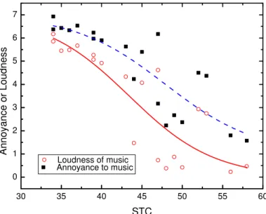
Figure 13 compares annoyance and loudness ratings of music sounds plotted versus STC values. Although the mean annoyance ratings are higher than the mean loudness ratings, the forms of the

regression lines are quite similar and the related R2 values are also very similar. As previously

described, the response scales were a little different in that the loudness responses included a 0 value to indicate inaudible speech or music sounds. These differences and the different source levels may explain the difference in average values of the loudness and annoyance responses.

0 1 2 3 4 5 6 7 30 35 40 45 50 55 60 Loudness of music Ann oy anc e or Loudn es s Annoyance to music STC

Figure. 13. Comparison of mean annoyance and mean loudness ratings plotted versus STC values for music sounds, [Annoyance, R2=0.728, Loudness, R2=0.734].

Figure 14 similarly compares annoyance and loudness ratings of speech sounds and shows very similar relationships between annoyance ratings and loudness ratings versus STC values for speech sounds. For both speech and music sounds the Boltzmann fits for annoyance and loudness responses have similar slopes at the mid-points of the curves as indicated by the similar dx values (see Table 4). The differences in overall average loudness and annoyance responses are to be expected due to the differences in response scales and source sound levels used. It is important to note that other than these obvious differences, annoyance and loudness responses are very

30 35 40 45 50 55 60 0 1 2 3 4 5 6 7 Annoyance to speech Annoy anc e or L oudnes s Loudness of speech STC

Figure 14. Comparison of mean annoyance and mean loudness ratings plotted versus STC values for speech sounds, [Annoyance, R2=0.856, Loudness, R2=0.886].

Figure 15 plots annoyance responses versus loudness responses. The near linear relationships and

high R2 values again indicate that these different concepts lead to quite similar results. That is,

sounds that are judged to be louder will usually be judged to be more annoying in these experiments. It is probably not necessary to assess both loudness and annoyance responses as they seem to provide essentially the same information.

1 2 3 4 5 6 7 0 1 2 3 4 5 6 7 1 2 3 4 5 6 7 Music Speech Annoy an c e Loudness

Figure 15. Relationship between mean annoyance and mean loudness ratings for both speech and music sounds, [Music, R2=0.957, Speech, R2=0.943]

4. Effects of Included Frequencies for Arithmetic Average TL Measures

4.1 More important frequencies for TL data

Correlation analyses were carried out between subjective responses from the annoyance and loudness tests and sound transmission loss (TL) values at each 1/3-octave band frequency for the 20 walls. Figures 16 shows the correlation coefficients between the two responses and TL values for the music sounds as a function of frequency. Similar results for the speech sounds are given in Figure 17. Although the results for annoyance and loudness response are very similar in each graph, there are large differences between the two graphs. That is, the frequencies most important for responses to music sounds are quite different than those most important for speech sounds. The dash-dotted line with cross symbols is the standard deviations of the wall TL values, Plotted according to the scale of the right hand axis so that they are more easily compared with the correlation coefficient values.

-1.0 -0.8 -0.6 -0.4 -0.2 0.0 63 125 250 500 1k 2k 4k Frequency, Hz Annoyance Loudness STDev of wall TL Correlat ion Coef fic ient 6 7 8 9 10 St andard Dev iat ion, dB

Figure 16. Correlation coefficients between mean annoyance and loudness ratings of music sounds and 1/3-octave band TL values. The standard deviations (STDev) of the wall TL values

are also plotted for comparison in terms of the right hand axis scale.

For the responses to music sounds in Figure 16, there is a strong similarity between the variations of the correlation coefficients and the variations of the standard deviations of TL values with frequency. This indicates that the correlations are stronger when there is more variation in the TL values. Figure 5 showed that the transmitted music spectra have higher levels and larger

variations in levels at low frequencies and to a lesser extent at high frequencies. Thus, for music, the low and high frequency TL values best predict the annoyance and loudness responses to the music sounds.

Compared to Figure 16, Figure 17 shows stronger correlation coefficients at mid-frequencies for the responses to speech sounds. Figure 6, showed that the spectra of the transmitted speech sounds had more prominent mid-frequency components than did the music sounds. Of course, it is well known that mid-and high frequency sounds contribute most to the intelligibility of speech and that lower frequency components, even when present are much less important for speech. Presumably, it is the same frequencies of transmitted speech sounds that contribute most to the annoyance and loudness responses to the speech sounds.

-1.0 -0.8 -0.6 -0.4 -0.2 0.0 63 125 250 500 1k 2k 4k Frequency, Hz Annoyance Loudness STDev of wall TL Correla ti on Coe ff ic ient 6 7 8 9 10 St andard Devi a tion, dB

Figure 17. Correlation coefficients versus frequency between mean annoyance and mean loudness ratings of speech sounds and 1/3-octave band TL values. The standard deviations (STDev) of the wall TL values are also plotted for comparison in terms of the right hand axis

scale.

4.2 Included frequencies for Arithmetic Averages TL values

In previous work [6], arithmetic averages of TL values over various frequency ranges were found to be good correlates of speech intelligibility scores. Table 5 shows correlation coefficients of annoyance ratings of music sounds with arithmetic averages of TL values over frequency ranges

from some lower frequency f1 to an upper frequency f2.

f1 f2 200 250 315 400 500 630 800 1000 1250 1600 2000 2500 3150 4000 5000 6300 63 -0.98 -0.98 -0.97 -0.95 -0.93 -0.90 -0.87 -0.84 -0.81 -0.79 -0.78 -0.8 -0.83 -0.85 -0.86 -0.87 80 -0.97 -0.96 -0.94 -0.91 -0.88 -0.84 -0.81 -0.77 -0.73 -0.71 -0.71 -0.74 -0.77 -0.80 -0.82 -0.84 100 -0.95 -0.93 -0.91 -0.87 -0.82 -0.78 -0.74 -0.70 -0.66 -0.64 -0.65 -0.69 -0.73 -0.76 -0.79 -0.81 125 -0.93 -0.89 -0.85 -0.80 -0.75 -0.70 -0.65 -0.60 -0.56 -0.54 -0.57 -0.62 -0.67 -0.71 -0.75 -0.77 160 -0.90 -0.84 -0.78 -0.71 -0.65 -0.60 -0.54 -0.50 -0.46 -0.44 -0.48 -0.54 -0.61 -0.66 -0.71 -0.74 200 -0.81 -0.72 -0.67 -0.59 -0.52 -0.47 -0.42 -0.38 -0.34 -0.34 -0.39 -0.47 -0.55 -0.62 -0.67 -0.71 250 -0.57 -0.57 -0.49 -0.42 -0.38 -0.33 -0.29 -0.26 -0.27 -0.33 -0.42 -0.51 -0.59 -0.65 -0.69 315 -0.56 -0.44 -0.37 -0.33 -0.28 -0.24 -0.21 -0.22 -0.29 -0.40 -0.50 -0.58 -0.64 -0.69 400 -0.31 -0.25 -0.24 -0.19 -0.16 -0.14 -0.16 -0.25 -0.37 -0.49 -0.58 -0.65 -0.70 500 -0.18 -0.20 -0.15 -0.11 -0.10 -0.12 -0.23 -0.38 -0.50 -0.60 -0.67 -0.72 630 -0.21 -0.13 -0.09 -0.07 -0.11 -0.24 -0.40 -0.54 -0.64 -0.71 -0.76 800 -0.04 -0.02 -0.02 -0.08 -0.24 -0.43 -0.58 -0.69 -0.75 -0.80 1000 0.00 -0.01 -0.10 -0.29 -0.49 -0.65 -0.75 -0.81 -0.84 1250 -0.03 -0.15 -0.36 -0.57 -0.72 -0.81 -0.86 -0.88 1600 -0.25 -0.47 -0.67 -0.80 -0.87 -0.90 -0.92 2000 -0.58 -0.77 -0.88 -0.92 -0.94 -0.95

Table 5. Correlation coefficients between AA(f1-f2) values and annoyance ratings of music

sounds. The lowest included frequency is f1 (shown in left hand column) and the highest included

frequency is f2 (top row). The shaded cells indicate values with magnitudes ≥0.90, and bold font

≥0.95.

These same correlation coefficients are plotted on the contour map of Figure 18 illustrating how

strongest correlations with responses to music sounds occur when low or high frequencies are included. 200 250 315 400 500 630 800 1000 1250 1600 2000 2500 3150 4000 5000 6300 63 80 100 125 160 200 250 315 400 500 630 800 1000 1250 1600 2000 0.00-0.05 -0.05-0.00 -0.10--0.05 -0.15--0.10 -0.20--0.15 -0.25--0.20 -0.30--0.25 -0.35--0.30 -0.40--0.35 -0.45--0.40 -0.50--0.45 -0.55--0.50 -0.60--0.55 -0.65--0.60 -0.70--0.65 -0.75--0.70 -0.80--0.75 -0.85--0.80 -0.90--0.85 -0.95--0.90 -1.00--0.95

Figure 18. Correlation coefficient between AA(f1-f2) and annoyance ratings of music sounds

(vertical axis lowest frequency f1, horizontal axis upper frequency f2).

f1 f2 200 250 315 400 500 630 800 1000 1250 1600 2000 2500 3150 4000 5000 6300 63 -0.67 -0.73 -0.79 -0.85 -0.89 -0.93 -0.95 -0.97 -0.98 -0.98 -0.98 -0.98 -0.97 -0.97 -0.96 -0.96 80 -0.74 -0.79 -0.85 -0.90 -0.93 -0.95 -0.97 -0.98 -0.98 -0.98 -0.98 -0.98 -0.98 -0.98 -0.98 -0.97 100 -0.78 -0.84 -0.89 -0.93 -0.95 -0.97 -0.98 -0.98 -0.98 -0.98 -0.98 -0.98 -0.98 -0.98 -0.98 -0.98 125 -0.85 -0.89 -0.93 -0.96 -0.97 -0.98 -0.97 -0.97 -0.96 -0.95 -0.96 -0.97 -0.98 -0.98 -0.99 -0.98 160 -0.89 -0.92 -0.95 -0.96 -0.96 -0.96 -0.95 -0.93 -0.92 -0.91 -0.93 -0.95 -0.97 -0.98 -0.98 -0.98 200 -0.90 -0.92 -0.94 -0.94 -0.93 -0.92 -0.90 -0.88 -0.87 -0.86 -0.89 -0.92 -0.95 -0.97 -0.98 -0.98 250 -0.90 -0.92 -0.91 -0.90 -0.88 -0.86 -0.84 -0.82 -0.82 -0.85 -0.89 -0.93 -0.96 -0.97 -0.98 315 -0.92 -0.90 -0.87 -0.86 -0.83 -0.81 -0.79 -0.79 -0.83 -0.88 -0.92 -0.95 -0.96 -0.97 400 -0.85 -0.82 -0.81 -0.78 -0.75 -0.73 -0.74 -0.79 -0.86 -0.91 -0.94 -0.96 -0.96 500 -0.77 -0.77 -0.74 -0.70 -0.69 -0.71 -0.77 -0.85 -0.90 -0.94 -0.95 -0.96 630 -0.78 -0.72 -0.68 -0.66 -0.69 -0.76 -0.84 -0.90 -0.94 -0.95 -0.95 800 -0.63 -0.61 -0.61 -0.65 -0.75 -0.84 -0.91 -0.93 -0.94 -0.94 1000 -0.58 -0.59 -0.66 -0.76 -0.85 -0.91 -0.93 -0.93 -0.93 1250 -0.60 -0.68 -0.77 -0.86 -0.91 -0.92 -0.92 -0.90 1600 -0.72 -0.78 -0.85 -0.89 -0.89 -0.89 -0.88 2000 -0.75 -0.83 -0.86 -0.86 -0.85 -0.84

Table 6. Correlation coefficient between AA(f1-f2) values and annoyance ratings of speech

sounds. The shaded cells indicate values with magnitudes ≥0.90, bold font ≥0.97.

f2Hz

Table 6 shows the results of correlating annoyance responses to speech sounds with arithmetic

average transmission loss values, AA(f1- f2), for a wide range of combinations of lower frequency

f1, and upper frequency f2 values. In contrast to responses to music sounds, for the annoyance

ratings of speech sounds, the highest correlations were obtained when mid-to-high frequency TL values were included. The same correlation coefficients between annoyance ratings of transmitted

speech sounds and AA(f1- f2) values are plotted in the contour plot of Figure 19. A number of

combinations yielded quite high correlation coefficients but simply including all 1/3-octave bands from 100 to 5k Hz is a successful combination and includes all frequencies assessed in standard transmission tests. Alternatively, including the speech frequencies from 160 Hz to 5k Hz is equally successful. 200 250 315 400 500 630 800 _{1000 1250 1600 2000 2500 3150 4000 5000 6300} 63 80 100 125 160 200 250 315 400 500 630 800 1000 1250 1600 2000 0-0.05 -0.05-0 -0.1--0.05 -0.15--0.1 -0.2--0.15 -0.25--0.2 -0.3--0.25 -0.35--0.3 -0.4--0.35 -0.45--0.4 -0.5--0.45 -0.55--0.5 -0.6--0.55 -0.65--0.6 -0.7--0.65 -0.75--0.7 -0.8--0.75 -0.85--0.8 -0.9--0.85 -0.95--0.9 -1--0.95

Figure 19. Correlation coefficients between AA(f1-f2) and annoyance ratings of speech sounds

(vertical axis lowest frequency f1, horizontal axis upper frequency f2).

The pattern of correlation coefficients in Figures 18 and 19 for annoyance responses was found to be very similar to the correlations between the same arithmetic average transmission loss values and loudness ratings. These are shown in Figures 20 and 21. The contours of correlation

coefficient values for loudness ratings of music sounds in Figure 20 are seen to be very similar to those in Figure 18 for annoyance ratings of music sounds. The results in Figure 21 for loudness ratings of speech sounds are very similar to those in Figure 19 for annoyance ratings of

transmitted speech sounds.

f2Hz

200 250 315 400 500 630 800 1000 1250 1600 2000 2500 3150 4000 5000 6300 63 80 100 125 160 200 250 315 400 500 630 800 1000 1250 1600 2000 0.05-0.1 0-0.05 -0.05-0 -0.1--0.05 -0.15--0.1 -0.2--0.15 -0.25--0.2 -0.3--0.25 -0.35--0.3 -0.4--0.35 -0.45--0.4 -0.5--0.45 -0.55--0.5 -0.6--0.55 -0.65--0.6 -0.7--0.65 -0.75--0.7 -0.8--0.75 -0.85--0.8 -0.9--0.85 -0.95--0.9 -1--0.95

Figure 20. Correlation coefficient between AA(f

- f

) and loudness ratings of music

sounds

.

200 250 315 400 500 630 800 1000 1250 1600 2000 2500 3150 4000 5000 6300 63 80 100 125 160 200 250 315 400 500 630 800 1000 1250 1600 2000 0-0.05 -0.05-0 -0.1--0.05 -0.15--0.1 -0.2--0.15 -0.25--0.2 -0.3--0.25 -0.35--0.3 -0.4--0.35 -0.45--0.4 -0.5--0.45 -0.55--0.5 -0.6--0.55 -0.65--0.6 -0.7--0.65 -0.75--0.7 -0.8--0.75 -0.85--0.8 -0.9--0.85 -0.95--0.9 -1--0.95

Figure 21. Correlation coefficient between AA(f

- f

) and loudness ratings of speech

sounds

4.3 Comparisons of some better Arithmetic Average TL measures Annoyance versus AA(100-5k)

The results in Table 6 suggest that an arithmetic average transmission loss over all of the

frequencies normally included in transmission loss tests (AA(100-5k)) would be strongly related to annoyance ratings of transmitted speech sounds. Annoyance responses to both speech and music sounds are plotted versus AA(100-5k) values in Figure 22. The annoyance ratings of

speech sounds are extremely strongly related to this measure with an associated R2 = 0.952.

However, this measure was less well related to the annoyance ratings of music sounds (R2=0.625).

f2Hz

30 35 40 45 50 55 60 1 2 3 4 5 6 7 Annoy anc e AA(100,5k), dB Music Speech not at all annoyed moderately annoyed extremely annoyed

Figure 22. Mean annoyance ratings of speech and music sounds versus AA(100-5k). [Music, R2=0.625, Speech, R2=0.952]

Annoyance versus AA(200-3.15k)

In the previous study [6,7] AA(200-2.5k) was best correlated with the speech intelligibility scores. When tested as a predictor of annoyance responses in the current work, this same measure

was strongly related to annoyance ratings of speech responses (R2 = 0.839) but only weakly

related to annoyance ratings of music ratings (R2 = 0.209)).

A slightly different arithmetic average transmission loss measure, AA(200-3.15k), was found to be a better compromise that was better related to annoyance ratings of speech ratings as well as being almost equally well related to the speech intelligibility scores of the previous study. Figure 23 plots annoyance responses versus AA(200-3.15k) values. Annoyance ratings of speech responses were again strongly related with the AA(200-3.15k) values but annoyance ratings of music responses were not well predicted.

The regression line for speech intelligibility scores from the previous study [6,7] is compared with the annoyance responses to speech sounds on Figure 23. The two regression lines have quite different slopes near their mid-points. That is, speech intelligibility scores vary more rapidly with AA(200-3.15k) values than do the ratings of annoyance ratings of speech. As a result, there is still reported annoyance when the intelligibility scores are close to ‘0’ because listeners can hear the speech sounds even when the words are not intelligible.

Another arithmetic average measure with a further expanded frequency range, AA(160-3.15k), was found to be a little better compromise for both speech intelligibility scores and annoyance ratings of speech sounds. When speech intelligibility scores were fitted to AA(160-3.15k) values

with a Boltzmann equation, the related R2 was 0.931 and when annoyance ratings of speech

35 40 45 50 55 60 65 1 2 3 4 5 6 7 Annoy anc e AA(200-3.15k), dB Annoyance Music Annoyance Speech Speech Intelligibility not at all annoyed moderately annoyed extremely annoyed 0 100 50 SI, %

Figure 23. Mean annoyance ratings versus AA(200-3.15k) compared with speech intelligibility scores (right hand axis) from previous study [6,7], [Music, R2=0.290, Speech, R2=0.892, Speech

intelligibility, R2=0. 948].

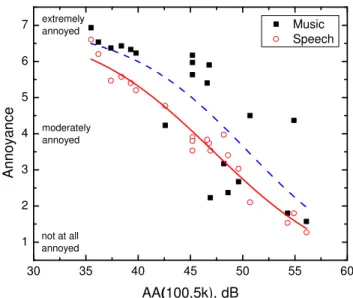
Annoyance versus AA(63-250) and AA(63-6.3k)

The results in Table 5 suggest that AA(63-250) should be well correlated with the annoyance ratings of music responses. The results in Figure 24 confirm that this measure was a good predictor of annoyance responses to music sounds and was also moderately well related to annoyance ratings of speech sounds.

By including a much broader range of frequencies, AA(63-6.3k) better includes all aspects of the transmission loss versus frequency characteristics including both very low and very high

frequencies. As the R2 values in the title of Figure 25 indicate, this measure was quite well

related to both annoyance ratings of speech and to music sounds. However, its success depended on the inclusion of frequencies that are not always included in standard sound transmission measurements. 10 15 20 25 30 35 40 1 2 3 4 5 6 7 Music Speech Annoy anc e AA(63-250) not at all annoyed moderately annoyed extremely annoyed

Figure 24. Mean annoyance ratings of speech and music sounds versus AA(63-250), [Music, R2=0.959, Speech, R2=0.531].

30 35 40 45 50 55 60 1 2 3 4 5 6 7 A n noyance AA(63-6.3k), dB Music Speech not at all annoyed moderately annoyed extremely annoyed

Figure 25. Mean annoyance ratings of speech and music sounds versus AA(63-6.3k) values. [Music, R2=0.788, Speech, R2=0.896]

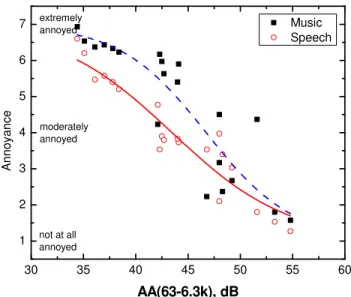
Loudness versus AA(200-3.15k) and AA(63-6.3k)

As shown in Figure 23, the arithmetic average transmission loss measure, AA(200-3.15k), was a good predictor of annoyance responses to speech sounds but was not so good for annoyance ratings of music responses. Figure 26 shows similar relationships with this measure for loudness ratings of transmitted speech and music sounds. The arithmetic average measure AA(63-6.3k) with an extended frequency range is related to loudness judgements in Figure 27. The results are similar to the plot of annoyance ratings versus this measure in Figure 25.

35 40 45 50 55 60 65 0 1 2 3 4 5 6 7 Music Speech Loudnes s AA(200-3.15k), dB not audible not at all loud moderately loud extremely loud

Figure 26. Mean loudness ratings of speech and music sounds versus AA(200-3.15k) values, [Music, R2=0.258, Speech, R2=0.832].

30 35 40 45 50 55 0 1 2 3 4 5 6 7 Loudnes s AA(63-6.3k), dB Music Speech not audible not at all loud moderately loud extremely loud

Figure 27. Mean loudness ratings of speech and music sounds versus AA(63-6.3k), [Music, R2=0.745, Speech, R2=0.919].

Table 7 compares the results of the Boltzmann equation fits of the loudness and annoyance responses with the more successful arithmetic average measures discussed above. As previously noted, some measures were better predictors of either responses to speech sounds or responses to music sounds but not responses to both types of sounds. As a compromise that predicts responses to both speech and music sounds, the AA(100-5k) measure was reasonably successful. However, the two arithmetic average measures that included low frequencies, 250) and AA(63-6.3k), were also possible compromises for both speech and music sounds.

The R2 values for annoyance responses were always very similar to those for the corresponding

loudness responses. Again loudness and annoyance responses seem to convey the same information about attitudes to these sounds.

Annoyance Loudness Symbol Type f1 f2 R2 X₀ dx R2 X₀ dx AA(100-5k) music 100 5k 0.625 48.522 4.974 0.593 44.769 5.149 speech 100 5k 0.952 45.154 5.310 0.944 41.358 5.602 AA(200-2.5k) music 200 2.5k 0.209 54.021 10.396 speech 200 2.5k 0.839 48.152 5.791 AA(200-3.15k) music 200 3.15k 0.290 53.277 8.507 0.258 47.710 8.790 speech 200 3.15k 0.892 48.380 5.471 0.832 44.555 5.793 AA(63-250) music 63 250 0.959 29.904 5.182 0.982 25.284 4.937 speech 63 250 0.531 25.161 9.811 0.648 19.993 8.016 AA(63-6.3k) music 63 6.3k 0.788 46.733 4.157 0.745 43.363 4.298 speech 63 6.3k 0.896 43.468 4.157 0.919 39.744 5.520

Table 7. Summary of regression results for better arithmetic average transmission loss measures. R2 values equal to or greater than 0.90 are shaded and R2 values equal to or greater than 0.95

4.4 Effects of included frequencies for Energy Average TL measures

Broadband transmission loss values were also created by energy averaging the measured transmission loss values over various frequency ranges rather than using arithmetic averages of these decibel values. The resulting correlation coefficients between these energy average transmission loss values and annoyance ratings of music responses are included in Table 8. In these results the lowest included frequency was varied from 63 Hz to 2000 Hz and the highest included frequency from 200 Hz to 6300 Hz.

f1 f2 200 250 315 400 500 630 800 1000 1250 1600 2000 2500 3150 4000 5000 6300 63 -.94 -.95 -.95 -.95 -.95 -.95 -.95 -.95 -.95 -.95 -.95 -.95 -.95 -.95 -.95 -.95 80 -.96 -.96 -.96 -.96 -.96 -.96 -.96 -.96 -.97 -.97 -.97 -.97 -.97 -.97 -.97 -.97 100 -.95 -.95 -.96 -.96 -.96 -.96 -.96 -.96 -.96 -.96 -.96 -.96 -.96 -.96 -.96 -.96 125 -.94 -.94 -.93 -.93 -.93 -.93 -.93 -.93 -.93 -.93 -.93 -.93 -.93 -.93 -.93 -.93 160 -.91 -.91 -.89 -.88 -.88 -.88 -.88 -.87 -.87 -.87 -.87 -.87 -.88 -.88 -.88 -.88 200 -.81 -.75 -.72 -.72 -.71 -.70 -.70 -.70 -.70 -.70 -.70 -.71 -.72 -.72 -.72 -.72 250 -.57 -.55 -.55 -.53 -.53 -.52 -.52 -.51 -.51 -.53 -.55 -.57 -.58 -.58 -.58 315 -.49 -.49 -.46 -.45 -.44 -.44 -.43 -.43 -.45 -.45 -.55 -.57 -.57 -.58 400 -.31 -.28 -.27 -.26 -.25 -.25 -.25 -.32 -.41 -.52 -.56 -.57 -.58 500 -.18 -.19 -.18 -.17 -.16 -.17 -.29 -.44 -.59 -.64 -.65 -.66 630 -.41 -.47 -.50 -.52 -.53 -.45 -.42 -.39 -.37 -.36 -.35 800 -.04 -.02 -.02 -.08 -.32 -.59 -.77 -.80 -.81 -.82 1000 -0.004 -.01 -.10 -.37 -.66 -.83 -.86 -.86 -.87 1250 -0.03 -.16 -.43 -.73 -.87 -.90 -.90 -.90 1600 -.25 -.50 -.79 -.91 -.93 -.93 -.94 2000 -.58 -.84 -.94 -.95 -.95 -.95

Table 8. Correlation coefficients between energy average transmission loss values over various frequency ranges from f1 to f2 with annoyance ratings of music sounds. The shaded values

indicate values with magnitudes ≥0.90, bold font ≥0.97.

f1 f2 200 250 315 400 500 630 800 1000 1250 1600 2000 2500 3150 4000 5000 6300 63 -.51 -.51 -.52 -.52 -.52 -.52 -.52 -.52 -.52 -.52 -.52 -.52 -.52 -.52 -.52 -.52 80 -.59 -.60 -.61 -.61 -.61 -.61 -.61 -.61 -.61 -.61 -.61 -.61 -.61 -.61 -.61 -.61 100 -.64 -.66 -.67 -.67 -.67 -.67 -.67 -.67 -.67 -.67 -.67 -.67 -.67 -.67 -.67 -.67 125 -.81 -.82 -.84 -.84 -.84 -.84 -.84 -.84 -.84 -.85 -.85 -.85 -.85 -.85 -.85 -.85 160 -.87 -.89 -.91 -.91 -.91 -.91 -.92 -.92 -.92 -.92 -.92 -.92 -.92 -.92 -.92 -.92 200 -.90 -.92 -.94 -.94 -.94 -.94 -.94 -.94 -.95 -.95 -.95 -.95 -.95 -.95 -.95 -.95 250 -.90 -.92 -.92 -.92 -.92 -.92 -.92 -.92 -.92 -.93 -.94 -.95 -.95 -.95 -.95 315 -.92 -.92 -.91 -.91 -.90 -.90 -0.90 -.90 -.91 -.93 -.95 -.96 -.96 -.96 400 -.85 -.83 -.83 -.82 -.82 -.82 -.82 -.85 -.89 -.94 -.96 -.96 -.96 500 -.77 -.77 -.76 -.75 -.75 -.76 -.82 -.88 -.95 -.96 -.97 -.97 630 -.89 -.92 -.94 -.94 -.95 -.92 -.90 -.89 -.88 -.88 -.87 800 -.63 -.62 -.62 -.66 -.76 -.88 -.94 -.95 -.95 -.94 1000 -.58 -.59 -.67 -.76 -.89 -.93 -.93 -.93 -.93 1250 -.60 -.69 -.76 -.89 -.92 -.91 -.91 -.91 1600 -.72 -.76 -.88 -.89 -.88 -.88 -.88 2000 -.75 -.86 -.86 -.85 -.85 -.85

Table 9. Correlation coefficients between energy averaged transmission loss values over various frequency ranges from f1 to f2 with annoyance ratings of speech sounds. The shaded values

The highest correlation coefficient values in Table 8 were similar to those for the corresponding arithmetic average transmission loss values in Tables 5. However, the range of included

frequencies that provided the strongest correlations were much wider than for the arithmetic averages in Table 5. For example, the results in Table 8 suggest that an energy average TL measure over the frequencies from 80 to 5k Hz would be a good predictor of annoyance ratings of music sounds.

Table 9 shows the results of correlations between energy averaged transmission loss values for

varied frequency range from f1 to f2 with annoyance ratings of speech sounds. The highest

correlation coefficient values were a little lower than those for the corresponding arithmetic average transmission loss values in Table 6.

5. Variations of STC Ratings

5.1 Variations of the 8 dB Rule

In the previous study [6,7], that used speech intelligibility scores to rate sound insulation, removing the 8 dB rule from the standard STC contour fitting procedure led to slightly improved predictions of intelligibility scores. Figure 28 shows the results of plotting annoyance responses

versus STC values with the 8 dB rule excluded. As the R2 values in the title of this figure

indicate, removing the 8 dB rule reduced the R2 values for annoyance ratings of music sounds but

increased R2 for annoyance ratings of speech sounds.

25 30 35 40 45 50 55 60 1 2 3 4 5 6 7 Annoy anc e STC_no8 Music Speech not at all annoyed moderately annoyed extremely annoyed

Figure 28. Mean annoyance ratings versus STCno8 values, [Music, R2=0.670 (0.728), Speech,

R2=0.950 (0.856)]. (Values in brackets are R2 with 8 dB rule included).

Figure 29 shows very similar results for loudness ratings of speech and music sounds in terms of STC values calculated without an 8 dB rule. As for the annoyance responses in Figure 28,

removing the 8 dB rule increased the R2 values for loudness ratings of speech sounds but reduced

them for loudness rating of music sounds.

25 30 35 40 45 50 55 60 0 1 2 3 4 5 6 7 Loudness STC_no8 Music Speech not audible not at all loud moderately loud extremely loud

Figure 29. Mean loudness ratings versus STCno8, [Music, R2=0.654 (0.734), Speech, R2=0.970

The previous research [6,7] found that including the 8 dB rule did not improve correlations with speech intelligibility scores and examined the benefits of varying the magnitude of the maximum allowed deviation from 8 dB to other values. Similar variations in the allowed magnitude of the maximum allowed deviation were also examined in this research. Figure 30 shows the results of correlations of mean loudness and annoyance ratings with STC values having varied maximum allowed deviation values.

Figure 30 shows, that annoyance and loudness ratings yielded very similar correlation

coefficients. However response to music sounds and responses to speech sounds led to different results. For music, the lower the maximum acceptable deficiency was, the higher the resulting correlation coefficient. The inverse was true for speech; the higher the magnitude of the

maximum acceptable deficiency, the higher the resulting correlation coefficient. For speech, the no 8 dB rule case led to the highest correlation coefficients because this was similar to a very large maximum allowed deficiency.

-1.0 -0.9 -0.8 -0.7 -0.6 no 1 2 3 4 5 6 7 8 9 10 12 14 16 Maximum deficiency, dB Correlat ion c oef fi c ient

Annoyance for music Annoyance for speech Loudness for music Loudness for speech

Figure 30. Correlation coefficients of STCno8 values (for varied maximum allowed deficiency)

with mean annoyance and loudness ratings for speech and music sounds.

Maximum Annoyance Loudness Deficiency music speech music speech

None -0.82 -0.98 -0.80 -0.97 1 -0.89 -0.90 -0.89 -0.91 2 -0.89 -0.90 -0.89 -0.91 3 -0.89 -0.90 -0.89 -0.91 4 -0.89 -0.90 -0.89 -0.91 5 -0.89 -0.90 -0.89 -0.91 6 -0.89 -0.90 -0.88 -0.91 7 -0.87 -0.92 -0.86 -0.92 8 -0.85 -0.94 -0.84 -0.94 9 -0.85 -0.95 -0.83 -0.95 10 -0.83 -0.96 -0.82 -0.96 12 -0.82 -0.98 -0.80 -0.97 14 -0.82 -0.98 -0.80 -0.97 16 -0.82 -0.98 -0.80 -0.97

Table 10. Correlation coefficients of STCno8 values (for varied maximum allowed deficiency) with

To better understand the results in Figure 30 and Table 10, the frequency at which the 8 dB rule was applied was determined for all walls where the STC rating was limited by the 8 dB rule. In all 12 cases for which the 8 dB rule was applied, it was applied at lower frequencies (125 to 250 Hz) and most often (9 walls) in the 125 Hz 1/3-octave band. For the walls included in this study, the 8 dB rule functioned to better represent the effects of low frequency dips in the TL versus frequency responses. Where there was a large dip and low frequency transmitted sounds could be unusually loud, the 8 dB rule limited the STC value so that it better indicated the effect of the reduced attenuation of the low frequency sounds. For the music sounds with strong low frequency components, including the 8 dB rule led to better sound insulation ratings that were better

correlated with subjective ratings of the music sounds. However, for speech sounds without strong low frequency sound components, including the 8 dB rule distorted the rating of the more important mid- and higher-frequency components of the transmitted speech sounds.

5.2 Variations of the Total Allowed Deviation

The effect of varying the allowed total deviation in the STC and Rw calculations was also

examined by varying it from the 32 dB limit included in both the STC and Rw procedures. This

was done for annoyance and loudness ratings of both speech and music sounds with and without the 8 dB rule included. Figure 31 plots the correlation of annoyance ratings for speech and music sounds versus the total allowed deviation used for cases with and without the 8 dB rule.

For speech without the 8 dB rule, a maximum deficiency corresponding to the current standard value of 32 dB works as well as almost any value. If the maximum deficiency was much smaller than 32 dB, then the correlations with annoyance ratings of speech sounds decreased because the STC rating became more influenced by prominent low frequency dips in the transmission loss versus frequency characteristics. However, for annoyance ratings of music sounds, without the 8 dB rule the opposite was true. The highest correlations occurred for the minimum total deficiency because then the prominent low frequency dips in the transmission loss versus frequency

characteristics most influenced the STC rating.

-1.0 -0.9 -0.8 -0.7 -0.6 0 10 20 30 32 34 40 50 60 Total deficiency, dB Correlation co e ffi ci en t

Annoyance for music(no 8 dB rule) Annoyance for speech(no 8 dB rule) Anoyance for music

Annoyance for speech

Figure 31. Correlation coefficients between mean annoyance ratings and modified STC values for which the total allowed deficiency was varied from 0 to 60 dB.

When the 8 dB rule was included, the results were a little different. For annoyance ratings of speech responses, the correlation coefficients increased until the total deficiency equalled 20 dB. Presumably at higher values the STC became more influenced by the application of the 8 dB rule because of prominent low frequency dips. Because these low frequency dips did not greatly

influence annoyance ratings of speech sounds, the correlation coefficients decreased for higher values of the allowed total deviation. Conversely for annoyance ratings of music sounds with the 8 dB rule included, the highest correlations occurred for a minimum allowed total deviation. In this case, the STC rating was determined totally by the low frequency dips in the transmission loss versus frequency characteristics.

-1.0 -0.9 -0.8 -0.7 -0.6 0 10 20 30 32 34 40 50 60 Total deficiency, dB Correlation co e ffi ci en t

Loudness for music(no 8 dB rule) Loudness for speech(no 8 dB rule) Loudness for music

Loudness for speech

Figure 32. Correlation coefficients between loudness ratings and modified STC values for which the total allowed deficiency was varied from 0 to 60 dB.

Total Annoyance Loudness

deficiency music speech music speech

0 -0.89 -0.90 -0.89 -0.91 10 -0.86 -0.94 -0.85 -0.96 20 -0.84 -0.97 -0.82 -0.97 30 -0.82 -0.98 -0.80 -0.97 32 -0.82 -0.98 -0.80 -0.97 34 -0.82 -0.98 -0.80 -0.96 40 -0.81 -0.98 -0.79 -0.97 50 -0.81 -0.98 -0.78 -0.97 Without 8 dB rule 60 -0.81 -0.98 -0.78 -0.97 0 -0.89 -0.90 -0.89 -0.91 10 -0.86 -0.94 -0.85 -0.96 20 -0.85 -0.95 -0.84 -0.95 30 -0.86 -0.94 -0.85 -0.94 32 -0.85 -0.94 -0.84 -0.94 34 -0.86 -0.93 -0.85 -0.93 40 -0.87 -0.92 -0.86 -0.92 50 -0.88 -0.91 -0.88 -0.92 With 8 dB rule 60 -0.88 -0.91 -0.88 -0.92

Table 11. Summary of correlation coefficients between subjective responses and STC values with varied total allowed deficiency both with and without the 8 dB rule.

Figure 32 plots the correlation coefficients between loudness ratings and STC values for which the allowed total deviation was varied. The results for loudness responses in Figure 32 follow the same trends as those for annoyance responses in Figure 31. The correlation coefficients from both figures are also listed in Table 11.

The 8 dB rule is seen to be useful because it includes the influences of low frequency dips in the transmission loss versus frequency characteristics resulting in better predictions of subjective responses to sounds with significant low frequency content such as music. Responses to speech sounds are better predicted without the 8 dB rule.

6. Variations of R

Measures

6.1 Evaluation of standard Spectrum Adaptation Terms

The ISO Rw procedure includes two types of spectrum adaptation terms that can be applied. The

C-type spectrum adaptation term is intended to better represent responses to pink spectrum

sounds and the Ctr-type correction is to improve the rating of outdoor sounds such as road traffic

noise, which have strong low frequency components. Both types of spectrum adaptation terms were evaluated for annoyance and loudness ratings of speech and music sounds.

Figure 33 plots annoyance responses versus Rw +C values. The resulting R2 values are included in

the title of this figure, as are the R2 values for regression analyses with the Rw measure without

any spectrum adaptation term (in brackets). Adding the C-type spectrum correction term degraded the strength of the prediction of annoyance ratings of speech sounds but increased the

R2 value for annoyance ratings of music sounds.

25 30 35 40 45 50 55 1 2 3 4 5 6 7 An no ya nce R_w+C Music Speech not at all annoyed moderately annoyed extremely annoyed

Figure 33. Mean annoyance ratings versus Rw+C, [Music, R2=0.918 (0.798),

Speech, R2=0.741 (0.890)].

(Values in brackets are R2 for Rw values without any spectrum adaptation term added).

20 25 30 35 40 45 50 1 2 3 4 5 6 7 An no ya nce R_w + C_{tr(100-3.15k)} Music Speech not at all annoyed moderately annoyed extremely annoyed

Figure 34. Mean annoyance ratings versus Rw+Ctr(100-3.15k), [Music, R2=0.950 (0.798),

Speech, R2=0.566 (0.890)].

Figure 34 shows plots of annoyance ratings versus Rw +Ctr(100-3.15k) values. The effects were

similar to those in Figure 33 except they were larger. Adding the Ctr(100-3.15k) type correction

increased the R2 for annoyance ratings of music sounds more than in Figure 33 and reduced the

R2 for annoyance ratings of speech sounds more than in Figure 33 compared to results for Rw

values without any spectrum adaptation term.

Figures 35 and 36 show plots of loudness ratings versus Rw +C and Rw +Ctr(100-3.15k) respectively. These results are very similar to those for annoyance responses. Adding either spectrum

adaptation term increased R2 values for responses related to music sounds and decreased R2

values for responses to speech sounds.

25 30 35 40 45 50 55 0 1 2 3 4 5 6 7 Lo udnes s R_w + C Music Speech not audible not at all loud moderately loud extremely loud

Figure 35. Mean loudness ratings versus Rw+C, [Music, R2=0.900 (0.779),

Speech, R2=0.821 (0.933)]. (Values in brackets are R2 values for loudness ratings versus Rw without any spectrum adaptation term added).

20 25 30 35 40 45 50 0 1 2 3 4 5 6 7 Lo udnes s R_w + C_{tr(100-3.15k)} Music Speech not audible not at all loud moderately loud extremely loud

Figure 36. Mean loudness ratings versus Rw+Ctr(100-3.15k), [Music, R2=0.960 (0.779),

Speech, R2=0.676 (0.933)]. (Values in brackets are R2 values for loudness ratings versus Rw

6.2 Evaluation of variations of Spectrum Adaptation Terms

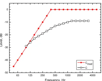
In the previous tests of speech intelligibility ratings [6,7], improved spectrum adaptation terms were found to increase the magnitude of correlations with intelligibility scores when added to the

Rw rating. Some correction terms were in the form of band pass filters that included only

frequencies important for speech intelligibility. Figure 37 illustrates the C200-3.15k spectrum

adaptation term that consists of a 0 dB attenuation (i.e. no attenuation) from 200 to 3.15k Hz and 50 dB attenuation outside of this frequency range.

-60 -50 -40 -30 -20 -10 0 10 63 125 250 500 1k 2k 4k Frequency, Hz Level, dB

Figure 37 Trial spectrum adaptation term response for speech (C200-3.15k).

Figure 38 plots mean annoyance responses versus Rw +C200-3.15k values. Figure 39 similarly plots

loudness responses versus values of the same measure, Rw +C200-3.15k. In Figure 38, this new

spectrum adaptation term led to a small increase in R2 values for responses to speech sounds

relative to those for just Rw values. Using this new spectrum adaptation term considerably

reduced R2 values for responses to music sounds relative to the R2 values for just Rw values.

Overall, this new spectrum adaptation term was not a very successful improvement for predicting loudness and annoyance ratings.

10 15 20 25 30 35 40 1 2 3 4 5 6 7 Annoy anc e R_w + C_200-3.15k Music Speech not at all annoyed moderately annoyed extremely annoyed

Figure 38. Mean annoyance ratings versus Rw+C200-3.15k, [Music, R2=0.508 (0.798), Speech,

10 15 20 25 30 35 40 0 1 2 3 4 5 6 7 Loudnes s R_w + C_200-3.15k Music Speech not audible not at all loud moderately loud extremely loud

Figure 39. Mean loudness ratings versus Rw+C200-3.15k, [Music, R2=0.521 (0.779), Speech,

R2=0.912 (0.933)].

(Values in brackets are R2 ratings for Rw).

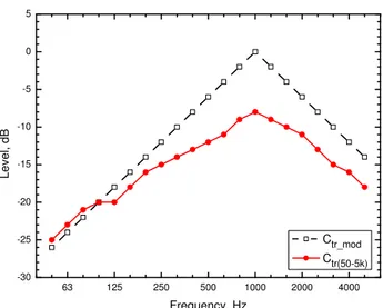
The ISO standard for Rw includes two variations of the Ctr spectrum adaptation term. One version

was considered in the results of Figures 34 and 36 (Rw+Ctr(100-3.15k)). It modifies the results at only the frequencies from 100 to 3.15k Hz. The other version modifies results at frequencies from 50 to 5k Hz and is illustrated in Figure 40.

Figures 41 and 42 plot annoyance and loudness responses respectively versus Rw +Ctr(50-5k) values.

Adding this spectrum adaptation term improves R2 values for annoyance and loudness ratings of

music sounds but decreases the R2 values for responses to speech sounds. Like the Ctr(100-3.15k)

spectrum adaptation term, this is only useful for responses to sounds with strong low frequency components such as music.

-30 -25 -20 -15 -10 -5 0 5 10 63 125 250 500 1k 2k 4k Frequency, Hz L evel, d B

20 25 30 35 40 45 50 1 2 3 4 5 6 7 Music Speech Annoy anc e R_w + C_tr(50-5k) not at all annoyed moderately annoyed extremely annoyed

Figure 41. Mean annoyance ratings versus Rw+Ctr(50-5k), [Music, R2=0.943 (0.798), Speech,

R2=0.388 (0.890)]. (Values in brackets are R2 for Rw).

20 25 30 35 40 45 50 0 1 2 3 4 5 6 7 Music Speech Loudnes s R_w + C_tr(50-5k) not audible not at all loud moderately loud extremely loud

Figure 42. Mean loudness ratings versus Rw+Ctr(50-5k). [Music, R2=0.980 (0.779), Speech,

R2=0.482 (0.933)]. (Values in brackets are R2 for Rw).

A modification of the Ctr spectrum adaptation term was created that simplified the shape of the