Mathematical Physics A Modem Introduction to Its Foundations pdf - Web Education

Sadri Hassani

Mathematical Physics

A Modem Introduction to

Its Foundations

With 152 Figures

,

Springer

ODTlJ KU1"UPHANESt

M. E. T. U. liBRARY

METULIBRARY

.. 2

~themltlcoJphysicS: Imodem

mllllllllllllllllllllllllllllll~11111111111111111111111111IIII

_002m7S69 QC20 H394

Sadri Hassani Department of Physics Illinois State University Normal, IL 61790 USA

hassani@entropy.phy.ilstu.edu

To my wife Sarah and to my children Dane Arash and Daisy Rita

336417

Libraryof Congress Cataloging-in-Publication Data Hassani, Sadri.

Mathematical physics: a modem introductionits foundations / Sadri Hassani.

p. em.

Includesbibliographical referencesand index. ISBN 0-387-98579-4 (alk. paper)

1. Mathematical physics. I.Title. QC20.H394 1998 530.15--<1c21 98-24738 Printed on acid-freepaper.

QC20

14394

c,2.

©1999Springer-Verlag New York, Inc.

All rights reserved.This work may not be translatedor copied in whole or in part without the written permission of the publisher (Springer-Verlag New York, Inc., 175 Fifth Avenue, New York, NY 10010, USA), except for brief excerpts in connection with reviews or scholarly analysis.Use-in connection with any form of informationstorage and retrieval, electronicadaptation, computer sctt-ware, or by similar or dissimilarmethodology now known or hereafterdevelopedis forbidden. The use of general descriptivenames, trade names, trademarks, etc., in this publication, evenifthe formerare not especiallyidentified, is not to be taken as a sign that such names, as understoodby the Trade Marks and Merchandise Marks Act, may accordinglybe used freely by anyone.

Productionmanagedby Karina Mikhli;manufacturing supervisedby ThomasKing. Photocomposed copy preparedfrom the author's TeX files.

Printed and bound by HamiltonPrinting Co., Rensselaer, NY. Printed in the United Statesof America.

9 8 7 6 5 4 3 (Correctedthird printing, 2002)

ISBN 0-387-98579-4 SPIN 10854281

Springer-Verlag New York Berlin: Heidelberg

Preface

"Ich kann es nun einmal nicht lassen, in diesem Drama von Mathematik und Physik---<lie sich im Dunkeln befrnchten,

aber von Angesicht zu Angesicht so geme einander verkennen und verleugnen-die Rolle des (wie ich gentigsam erfuhr, oft unerwiinschten)Botenzu spielen."

Hermann Weyl

Itis said that mathematics is the language of Nature.Ifso, then physics is its poetry. Nature started to whisper into our ears when Egyptians and Babylonians were compelled to invent and use mathematics in their day-to-day activities. The faint geomettic and arithmetical pidgin of over four thousand years ago, snitable for rudimentary conversations with nature as applied to simple landscaping, has turned into a sophisticated language in which the heart of matter is articulated.

The interplay between mathematics and physics needs no emphasis. What may need to be emphasized is that mathematics is not merely a tool with which the presentation of physics is facilitated, butthe only medium in which physics can survive. Just as language is the means by which humans can express their thoughts and without which they lose their unique identity, mathematics is the only language through which physics can express itself and without which it loses its identity. And just as language is perfected due to its constant usage, mathematics develops in the most dramatic way because of its usage in physics. The quotation by Weyl above, an approximation to whose translation is"In this drama of mathematics and physics-which fertilize each other in the dark, but which prefer to deny and misconstrue each other face to face-I cannot, however, resist playing the role of a messenger, albeit, as I have abundantly learned, often an unwelcome one:'

vi PREFACE

is a perfect description of the natnral intimacy between what mathematicians and physicists do, and the nnnatnral estrangement between the two camps. Some of the most beantifnl mathematics has been motivated by physics (differential eqnations by Newtonian mechanics, differential geometry by general relativity, and operator theory by qnantnmmechanics), and some of the most fundamental physics has been expressed in the most beantiful poetry of mathematics (mechanics in symplectic geometry, and fundamental forces in Lie group theory).

I do uot want to give the impression that mathematics and physics cannot develop independently. On the contrary, it is precisely the independence of each discipline that reinforces not only itself, but the other discipline as well-just as the stndy of the grammar of a language improves its usage and vice versa. However, the most effective means by which the two camps can accomplish great success is throngh an inteuse dialogue. Fortnnately, with the advent of gauge and string theories ofparticle physics, such a dialogue has been reestablished between physics and mathematics after a relatively long lull.

Level and Philosophy of Presentation

This is a book for physics stndeuts interested in the mathematics they use. It is also a book furmathematics stndeuts who wish to see some of the abstract ideas with which they are fantiliar come alive in an applied setting. The level of preseutation is that of an advanced undergraduate or beginning graduate course (or sequence of courses) traditionally called "Mathematical Methods of Physics" or some variation thereof. Unlike most existing mathematical physics books intended for the same audience, which are usually lexicographic collections of facts about the diagonalization of matrices, tensor analysis, Legendre polynomials, contour integration, etc., with little emphasis on formal and systematic development of topics, this book attempts to strike a balance between formalism and application, between the abstract and the concrete.

I have tried to include as mnch of the essential formalism as is necessary to render the book optimally coherent and self-contained. This entails stating and proving a large nnmber of theorems, propositions, lemmas, and corollaries. The benefit of such an approach is that the stndent will recognize clearly both the power and the limitation of a mathematical idea used in physics. There is a tendency on the part of the uovice to universalize the mathematical methods and ideas eucountered in physics courses because the limitations of these methods and ideas are not clearly pointed out.

There is a great deal of freedom in the topics and the level of presentation that instructors can choose from this book. My experience has showu that Parts I,TI, Ill, Chapter 12, selected sections of Chapter 13, and selected sections or examples of Chapter 19 (or a large snbset of all this) will be a reasonable course content for advanced undergraduates.Ifone adds Chapters 14 and 20, as well as selected topics from Chapters 21 and 22, one can design a course snitable for first-year graduate

PREFACE vii

students. By judicious choice of topics from Parts VII and VIII, the instructor can bring the content of the course to a more modern setting. Depending on the sophistication of the students, this can be done either in the first year or the second year of graduate school.

Features

To betler understand theorems, propositions, and so forth, students need to see them in action. There are over 350 worked-out examples and over 850 problems (many with detailed hints) in this book, providing a vast arena in which students can watch the formalism unfold. The philosophy underlying this abundance can be summarized as''Anexample is worth a thousand words of explanation." Thus, whenever a statement is intrinsically vague or hard to grasp, worked-out examples and/or problems with hints are provided to clarify it. The inclusion of such a large number of examples is the means by which the balance between formalism and application has been achieved. However, although applications are essential in understanding mathematical physics, they are only one side of the coin. The theorems, propositions, lemmas, and corollaries, being highly condensed versions of knowledge, are equally important.

A conspicuous feature of the book, which is not emphasized in other compa-rable books, is the attempt to exhibit-as much as.it is useful and applicable-« interrelationships among various topics covered. Thus, the underlying theme of a vector space (which, in my opinion, is the most primitive concept at this level of presentation) recurs throughout the book and alerts the reader to the connection between various seemingly unrelated topics.

Another useful feature is the presentation of the historical setting in which men and women of mathematics and physics worked. I have gone against the trend of the "ahistoricism" of mathematicians and physicists by summarizing the life stories of the people behind the ideas. Many a time, the anecdotes and the historical circumstances in which a mathematical or physical idea takes form can go a long way toward helping us understand and appreciate the idea, especiallyif the interaction among-and the contributions of-all those having a share in the creation of the idea is pointed out, and the historical continuity of the development of the idea is emphasized.

To facilitate reference to them, all mathematical statements (definitions, theo-rems, propositions, lemmas, corollaries, and examples) have been nnmbered con-secutively within each section and are preceded by the section number. For exam-ple, 4.2.9 Definition indicates the ninth mathematical statement (which happens to be a definition) in Section 4.2. The end of a proof is marked by an empty square D, and that of an example by a filled square III, placed at the right margin of each. Finally, a comprehensive index, a large number of marginal notes, and many explanatory underbraced and overbraced comments in equations facilitate the use

viii PREFACE

and comprehension of the book.Inthis respect, the book is also nsefnl as a refer-ence.

Organization and Topical Coverage

Aside from Chapter 0, which is a collection of pnrely mathematical concepts, the book is divided into eight parts. Part I, consisting of the first fonr chapters, is devoted to a thorough study of finite-dimensional vector spaces and linear operators defined on them. As the unifying theme of the book, vector spaces demand careful analysis, and Part I provides this in the more accessible setting of finite dimension in a language thatis conveniently generalized to the more relevant infinite dimensions,' the subject of the next part.

Following a brief discussion of the technical difficulties associated with in-finity, Part IT is devoted to the two main infinite-dimensional vector spaces of mathematical physics: the classical orthogonal polynomials, and Foutier series and transform.

Complex variables appear in Partill.Chapter 9 deals with basic properties of complex functions, complex series, and their convergence. Chapter 10 discusses the calculus of residues and its application to the evaluation of definite integrals. Chapter II deals with more advanced topics such as multivalued functions, analytic continuation, and the method of steepest descent.

Part IV treats mainly ordinary differential equations. Chapter 12 shows how ordinary differential equations of second order arise in physical problems, and Chapter 13 consists of a formal discussion of these differential equations as well as methods of solving them numerically. Chapter 14 brings in the power of com-plex analysis to a treatment of the hypergeometric differential equation. The last chapter of this part deals with the solution of differential equations using integral transforms.

Part V starts with a formal chapter on the theory of operator and their spectral decomposition in Chapter 16. Chapter 17 focuses on a specific type of operator, namely the integral operators and their corresponding integral equations. The for-malism and applications of Stnrm-Liouville theory appear in Chapters 18 and 19, respectively.

The entire Part VI is devoted to a discussion of Green's functions. Chapter 20 introduces these functions for ordinary differential equations, while Chapters 21 and 22 discuss the Green's functions in an m-dimensional Euclidean space. Some of the derivations in these last two chapters are new and, as far as I know, unavailable anywhere else.

Parts VII and

vrn

contain a thorough discussion of Lie groups and their ap-plications. The concept of group is introduced in Chapter 23. The theory of group representation, with an eye on its application in quantom mechanics, is discussed in the next chapter. Chapters 25 and 26 concentrate on tensor algebra and ten-, sor analysis on manifolds.In Part

vrn,

the concepts of group and manifold are

PREFACE ix

brought together in the coutext of Lie groups. Chapter 27 discusses Lie groups and their algebras as well as their represeutations, with special emphasis on their application in physics. Chapter 28 is on differential geometry including a brief introduction to general relativity. Lie's original motivation for constructing the groups that bear his name is discussed in Chapter 29 in the context of a systematic treatment of differential equations using their symmetry groups. The book ends in a chapter that blends many of the ideas developed throughout the previous parts in order to treat variational problems and their symmetries.Italso provides a most fitting example of the claim made at the beginning of this preface and one of the most beautiful results of mathematical physics: Noether's theorem ou the relation between symmetries and conservation laws.

Acknowledgments

Itgives me great pleasure to thank all those who contributed to the making of this book. George Rutherford was kind enough to voluuteer for the difficult task of condensing hundreds of pages of biography into tens of extremely informative pages. Without his help this unique and valuable feature of the book would have been next to impossible to achieve. Ithankhim wholeheartedly. Rainer Grobe and Qichang Su helped me with my rusty computational skills. (R. G. also helped me with my rusty German!) Many colleagues outside my department gave valuable comments and stimulating words of encouragement on the earlier version of the book. I wouldliketo record my appreciation to Neil Rasband for reading part of the manuscript and commenting on it. Special thanks go to Tom von Foerster, senior editor of physics and mathematics at Springer-Verlag, not ouly for his patience and support, but also for the,extreme care he took in reading the entire manuscript and giving me invaluable advice as a result. Needless to say, the ultimate responsibility for the content of the book rests on me. Last but not least, I thank my wife, Sarah, my son, Dane, and my daughter, Daisy, for the time taken away from them while I was writing the book, and for their support during the long and arduous writing

process.

Many excellent textbooks, too numerous to cite individually here, have influ-enced the writing of this book. The following, however, are noteworthy for both their excellence and the amount of their influence:

Birkhoff, G.,andG.-C. Rota, Ordinary Differential Equations, 3rd ed., New York, Wiley, 1978.

Bishop, R., and S. Goldberg, Tensor Analysis on Manifolds, New York, Dover, 1980.

Dennery, P., andA.Krzywicki, Mathematics for Physicists, New York, Harper& Row, 1967.

Halmos, P., Finite-Dimensional Vector Spaces, 2nd ed., Princeton, Van Nostrand, 1958.

x

PREFACE

Hamennesh, M. Group Theory and its Application to Physical Problems, Dover, New York, 1989.

Olver, P.Application ofLie Groups to Differential Equations, New York, Springer-Verlag, 1986.

Unless otherwise indicated, all biographical sketches have been taken from the following three sources:

Gillispie, C., ed., Dictionary ofScientific Biography, Charles Scribner's, New York, 1970.

Simmons, G. Calculus Gems, New York, McGraw-Hill, 1992. History of Mathematics archive at www-groups.dcs.st-and.ac.uk:80.

I wonld greatly appreciate any comments and suggestions for improvements. Although extreme care was taken to correctall the misprints, the mere volume of the book makes it very likely that I have missed some (perhaps many) of them. I shall be most grateful to those readers kind enough to bring to my attention any remaining mistakes, typographical or otherwise. Please feel free to contact me.

Sadri Hassani Campus Box 4560 Department of Physics Illinois State University Normal, IL 61790-4560, USA e-mail: hassani@entropy.phy.i1stu.edu

Itis my pleasure to thankall those readers who pointed out typographical mistakes and suggested a few clarifying changes. With the exceptionofa couple that required substantial revisiou, I have incorporated all the corrections and suggestions in this second printing.

Note to the Reader

Mathematics and physics arelike the game of chess (or, for that matter, like any gamej-i-you willleam only by ''playing'' them. No amount of reading about the game will make you a master.Inthis book you will find a large number of examples and problems. Go through as many examples as possible, and try to reproduce them. Pay particular attention to sentences like "The reader may check . .. "or"Itis straightforwardto show . .. "These are red flags warning you that for a good understanding of the material at hand, yon need to provide the missing steps. The problems often fill in missing steps as well; and in this respect they are essential for a thorough understanding of the book. Do not get discouraged if you cannot get to the solution of a problem at your first attempt. Ifyou start from the beginning and think about each problem hard enough, youwill get to the solution, .and you will see that the subsequent problems will not be as difficult.

The extensive index makes the specific topics about which you may be in-terested to leam easily accessible. Often the marginal notes will help you easily locate the index entry you are after.

I have included a large collection of biographical sketches of mathematical physicists of the past. These are truly inspiring stories, and I encourage you to read them. They let you see that even under excruciating circumstances, the human mind can work miracles. You will discover how these remarkable individuals overcame the political, social, and economic conditions of their time to let us get a faint glimpse of the truth. They are our true heroes.

1

1

1

1

1

1

1

1

1

1

1

1

1

1

1

1

1

1

1

1

1

1

1

1

1

1

1

Contents

Preface

Note to the Reader

List of Symbols

o

Mathematical Preliminaries 0.1 Sets . 0.2 Maps . 0.3 Metric Spaces . 0.4 Cardinality... 0.5 Mathematical Induction 0.6 P r o b l e m s . . . .

I

Finite-Dimensional Vector Spaces

1 Vectors and Transformations 1.1 Vector Spaces . . . . . 1.2 Inner Product . 1.3 Linear Transformations . 1.4 Algebras. 1.5 Problems... 2 Operator Algebra 2.1 Algebra

«s:

(V) v xi xxi 1 1 4 7 10 12 14

17

19

19

23

32

41 44

49

49

xiv

CONTENTS

2.2 Derivatives of Functions of Operators . 2.3 Conjugation of Operators . . . . 2.4 Hermitian and Unitary Operators 2.5 Projection Operators . . . . 2.6 OperatorsinNumerical Analysis 2.7 Problems...

3 Matrices: Operator Representations 3.1 Matrices... 3.2 Operations on Matrices .. . . . .

3.3 Orthonormal Bases .

3.4 Change of Basis and Similarity Transformation . 3.5 The Determinant . . .. 3.6 The Trace 3.7 Problems... 4 Spectral Decomposition 4.1 Direct Sums . . . . 4.2 InvariantSubspaces . . . . 4.3 Eigeuvaluesand Eigenvectors . 4.4 Spectral Decomposition 4.5 Functions of Operators 4.6 Polar Decomposition 4.7 Real VectorSpaces 4.8 Problems...

IT

Infinite-Dimensional Vector Spaces

5 Hilbert Spaces

5.1 The Question of Convergence . 5.2 The Space of Square-IntegrableFunctions 5.3 Problems...

6 Generalized Functions 6.1 ContinuousIndex 6.2 Generalized Functions . 6.3 Problems...

7 Classical Orthogonal Polynomials 7.1 General Properties . . 7.2 Classification... 7.3 Recurrence Relations . . . .

7.4 Examples of Classical Orthogonal Polynomials.

56 61 63

67

70

76

82

82

87

89

91 93

101

103

109

109 112 114 117 125 129 130 138

143

145 145 150 157

159

159 165 169

172

172 175 176 179

7.5 7.6 7.7

Expansion in Terms of Orthogonal Polynomials .. Generating Functions . . . . Problems . CONTENTS

xv

186 190 190 8 FourierAnalysis 8.1 Fourier Series . . . . . 8.2 The Fourier Transform . 8.3 Problems...

III

Complex Analysis

196 196 208 220

225

9 Complex Calculus 227 9.1 Complex Functions " 227 9.2 Analytic Functions. . . " 228 9.3 Conformal Maps .. . . 236 9A Integration of Complex Functions . . . " 241

9.5 Derivativesas Integrals 248

9.6 Taylor and Laurent Series . 252

9.7 P r o b l e m s . . . 263

10 Calculus of Residues

10.1 Residues . . . . 10.2 Classification of Isolated Singularities 10.3 Evaluation of Definite Integrals . . ..

lOA Problems .

11 Complex Analysis: AdvancedTopics ILl Meromorphic Functions . . . 11.2 Multivalued Functions . . . . 11.3 Analytic Continuation . . . . 1104 The Gamma and Beta Functions. . . . 11.5 Method of Steepest Descent . . . . 11.6 Problems. . . . 270 270 273 275 290 293 293 295 302 309 312 319

IV

DifferentialEquations

325

12 Separation of Variables in Spherical Coordinates 327

12.1 PDEs of Mathematical Physics .. . . 327 12.2 Separation oftheAngular Part of the Laplacian. . . .. 331 12.3 Construction of Eigenvalues ofL2. . . 334 1204 Eigenvectors of L2: Spherical Harmonics . . 338 12.5 Problems.. . . ., . . . 346

xvi CONTENTS

13 Second-Order Linear Differential Equations 348

13.1 General Properties of ODEs. . . 349 13.2 Existence and Uniqneness for First-Order DEs . 350

13.3 General Properties of SOLDEs . . . 352

13.4 The Wronskian. . . 355

13.5 Adjoint Differential Operators. . . . 364

13.6 Power-Series Solntions of SOLDEs . 367

13.7 SOLDEs with Constant Coefficients 376

13.8 The WKB Method . . . 380

13.9 Numerical Solntions of DEs . . . 383

13.10 Problems. . . 394

14 Complex Aualysis of SOLDEs 400

14.1 Analytic Properties of Complex DEs 401

14.2 Complex SOLDEs . . . 404

14.3 Fuchsian Differential Equations . . . 410

14.4 The Hypergeometric Functiou . . . . 413

14.5 Confiuent Hypergeometric Functions 419

14.6 Problems. . . 426

15 Integral Transforms and Differential Equations 433

15.1 Integral Representation of the Hypergeometric Function . . 434 15.2 Integral Representation of the Confiuent Hypergeometric

Function . . . 437

15.3 Integral Representation of Bessel Functions 438

15.4 Asymptotic Behavior of Bessel Functions. 443

15.5 Problems.. . . 445

V Operators on Hilbert Spaces

16 AnInlroduction to Operator Theory

16.1 From Abstract to Integral and Differential Operators . 16.2 Bounded Operators in Hilbert Spaces . .

16.3 Spectra of Linear Operators . .

16.4 Compact Sets .

16.5 Compact Operators .

16.6 Spectrum of Compact Operators

16.7 Spectral Theorem for Compact Operators . 16.8 Resolvents 16.9 Problems. . . . 17 Integral Equations 17.1 Classification.

449

451 451 453 457 458 464 467 473 480 485 488 488

CONTENTS xvii

17.2 Fredholm Integra!Equations . 494

17.3 Problems... 505

18 Sturm-Liouville Systems: Formalism 507

18.1 Unbounded Operators with Compact Resolvent 507 18.2 Sturm-Liouville Systems and SOLDEs . . . . 513 18.3 Other Properties of Sturm-Liouville Systems . 517 18.4 Problems. . . 522

19 Sturm-Lionville Systems: Examples 524

19.1 Expansions in Terms of Eigenfunctions . 524 19.2 Separation in Cartesian Coordinates. . . 526 19.3 Separation in Cylindrical Coordinates. . 535

19.4 Separation in Spherical Coordinates. 540

19.5 Problems... 545

VI

Green's Functions

20 Green's FunctionsinOne Dimension

20.1 Calculationof Some Green's Functions . 20.2 Formal Considerations . . . . 20.3 Green's Functions for SOLDOs . . . . . 20.4 EigenfunctionExpansion of Green's Fnnctions .

20.5 Problems.. . . .

21 Multidimensional Green's Functions: Formalism 21.1 Properties of Partial Differential Equations . 21.2 MultidimensionalGFs and Delta Functions . 21.3 Formal Development . . .

21.4 Integral Equations and GFs 21.5 Perturbation Theory 21.6 Problems. . . .

22 Multidimensional Green's Functions: Applications 22.1 Elliptic Equations . .

22.2 Parabolic Equations . . . . 22.3 HyperbolicEquations . . . . 22.4 The Fourier TransformTechnique . . . . 22.5 The EigenfunctionExpansion Technique 22.6 Problems. .. .. .. .. .. .. . . . .

551

553 r-554 557 565 577 580 583 584 592 596 600 603 610 613 613 621 626 628 636 641

xviii CONTENTS

VII

Groups and Manifolds

23 Group Theory 23.1 Groups. 23.2 Subgroups . . . 23.3 Group Action .

23.4 The Symmetric Group

s,

23.5 Problems. . . .

24 Group Representation Theory 24.1 Definitions and Examples 24.2 Orthogonality Properties. . . 24.3 Analysis of Representations . .

24.4 Group Algebra . . . .. . . . 24.5 Relationship of Characters to Those of a Subgroup . 24.6 Irreducible Basis Functions . . . .

24.7 Tensor Product of Representations . . . 24.8 Representations of the Symmetric Group 24.9 Problems.. .. .. .. . .. .. .. ..

25 Algebra of Tensors 25.1 Multilinear Mappings 25.2 Symmetries of Tensors . 25.3 Exterior Algebra . . . . . 25.4 hmer Product Revisited . 25.5 The Hodge Star Operator 25.6 Problems. . . .

26 Analysis of Tensors

26.1 Differentiable Manifolds. . 26.2 Curves and Tangent Vectors . 26.3 Differential of a Map . . . 26.4 Tensor Fields on Manifolds 26.5 Exterior Calculus . . . 26.6 Symplectic Geometry 26.7 Problems. . . .

VIII

Lie Groups and Their Applications

27 Lie Groups and Lie Algebras

27.1 Lie Groups and Their Algebras . . . . 27.2 An Outline of Lie Algebra Theory . . . 27.3 Representation of Compact Lie Groups . . .

649

651

652 656 663 664 669

673

-J 673 680 685 687 692 695 699 707 723

728

729 736 739 749 756 758

763

763 770 776 780 791 801 808

813

815

815 833 845

27.4 Representationof the General Linear Group . 27.5 Representationof Lie Algebras

27.6 Problems . CONTENTS xix 856 859 876 28 DifferentialGeometry 882

28.1 VectorFields and Curvature . . . 883

28.2 Riemannian Manifolds. . . . 887

28.3 CovariantDerivative and Geodesics . 897

28.4 Isometries and Killing VectorFields 908

28.5 Geodesic Deviation and Curvature . 913

28.6 General Theory of Relativity 918

28.7 Problems. . . 932

29 Lie GronpsandDifferentialEquations 936 29.1 Synunetries of Algebraic Equations. . . 936 29.2 Synunetry Groups of Differential Equations 941

29.3 The Central Theorems. . . 951

29.4 Application to Some Known PDEs 956

29.5 Application to ODEs. 964

29.6 Problems. . . 970

30 Calcnlusof Variations, Symmetries,andConservationLaws 973

30.1 The Calculus of Variations. . . 973 30.2 Symmetry Groups of VariationalProblems . . . 988 30.3 ConservationLaws and Noether's Theorem. . . 992 30.4 Application to Classical Field Theory . 997 30.5 Problems. . . .. 1000

Bibliography 1003

I

j

j

j

j

j

j

j

j

j

j

j

j

j

j

j

j

j

j

j

j

j

j

j

j

j

j

j

j

j

j

j

j

j

j

j

J

List of Symbols

E,(11')

z

R R+ C l\I

ill

~A

AxB

An U,

«»

A=B

x ... f(x) V 3 [a] gof

iff

ek(a, b) Cn(orJRn) pClt] P'[t] P~[t] Coo (al b)

lIall

"belongs to", ("does not belong to") Set of integers

Set of real nnmbers Set of positive real nnmbers Set of complex nnmbers Set of nonnegative integers Set of rational nnmbers Complement of the setA

Set of ordered pairs (a,b)witha E A andbE B

{(aI, a2, ... , an)lat E

Al

Union, (Intersection)

Ais eqnivalent toB

x is mapped to f(x) via the map f forall (valnes of)

There exists (a valne of)

Eqnivalence class to which

a

belongs Composition of maps

f

andg ifand only if

Set of functions on (a,b)with continnons derivatives np to orderk

Set of complex (or real) n-tnples

Set of polynomials intwith complex coefficients Set of polynomials intwith real coefficients

Set of polynomials with complex coefficients of degree

n

or less Set ofall complex seqnences(atl~1 snch that L:~I

latl

2_{< 00} Inner prodnct ofla) and

Ibl

xxii LIST OF SYMBOLS £-(V) [8,T] Tt At,or

A

l.lE/lV 8(x - xo) Res[f(zolJ DE, ODE, PDE SOLDE GL(V) GL(n,q SL(n,q 71 ®72 AJ\B AP(V)

Set of endomorphisms (linear operators) on vector space V Commutator of operators 8 and T

Adjoint (hermitian conjugate) of operator T Transpose of matrixA

Direct sum of vector spaces1.land V

Dirac delta function nonvanishing only atx = xo Residue of

f

at point zo

Differential equation, Ordinary DE, Partial DE Second order linear (ordinary) differential equation Set ofall invertible operators on vector space V

Set ofallnx ncomplex matrices of nonzero determinant Set ofallnx ncomplex matrices of unit determinant Tensor product of71 and72

Exterior (wedge) product of skew-symmetric tensors A and B Set ofall skew-symmetric tensors of type(p,0) on V

0

_

Mathematical Preliminaries

This introductory chapter gathers together some of the most basic tools and notions that are used throughout the book. Italso introduces some common vocabulary and notations used in modem mathematical physics literature. Readers familiar

with such concepts as sets, maps, equivalence relations, and metric spaces may

wish to skip this chapter.

0.1. Sets

Modem mathematics starts with the basic (and undefinable) concept of set. We think of a set as a structureless family, or collection, of objects. We speak, for example, of the set of students in a college, of men in a city, of women working concept ofset for a corporation, of vectors in space, of points in a plane, or of events in the elaborated continuum of space-time. Each member a of a set A is called an element of that sel. This relation is denoted bya E A (read"ais an element of A" or"abelongs toA"),and its negation by a ¢ A.Sometimes a is called a point of the setAto emphasize a geometric connotation.

A set is usually designated by enumeration of its elements between braces. For example, {2, 4, 6, 8} represents the set consisting of the first four even natural numbers; {O, ±I, ±2, ±3, ... } is the set of all integers; {I,x, x2,x 3, ... }is the set of all nonnegative powers ofx;and {I,i, -1, -i}is the set of the four complex fourth roots of unity.Inmany cases, a set is defined by a (mathematical) statement that holds for all ofits elements. Such a set is generally denoted by{x

I

P(x)}and read "the set of allx's such that P(x)is true." The foregoing examples of sets can be written alternatively as follows:

2 O. MATHEMATICAL PRELIMINARIES

{±n

I

nis a natural number}

{y

I

y = x" and n is a uatural uumber}

{z

I

Z4 = I andzis a complex uumber}

singleton (proper) subset empty set union, intersection, complement universal set Cartesian product ordered pairs

In a frequently used shorthand uotation, the last two sets can be abbreviated as [x"

I

n 2:

a

andn is an integer} and [z E iC

I

Z4 = I}. Similarly, the uuit circle can be deuoted by {z[z]= I}, the closed interval [a, b] as {xla ::; x ::; b},the open interval(a,b) as{x

I

a < x < b},and the set of all nonnegative powers of x as{x"}~o'This last notation will be used frequeutly iu this book. A set with a single element is called a singleton.

Ifa E A wheneveraE B,we say thatB is a subset ofA and write B C A or A:JB.IfBeA and A

c

B,thenA = B.1f BeA and A

i'

B, thenBis called a proper subset ofA.The set defined by{ala

i'

a}iscalled the empty set and is denoted by 0. Clearly, 0 contains no elements and is a subset of any arbitrary set. The collection of all subsets (including 0) of a set A is denoted by 2A•The reason for this notation is that the number of subsets of a set containingn elements is 2" (Problema.I).1fA and B are sets, their union, denoted by A U B, is the set containing all elements that belong toAorBor both. The intersection of the sets

.!\

and B,denoted byA n B,is the set containing all elements belonging to both

Aand B.If{B.}.El is a collection of sets,1we denote their union byU.B.and their intersection by

n.

B

a-Inany application of set theory there is an underlying universal set whose subsets are the objects of study. This universal set is usually clear from the context. For exaunple, in the study of the properties of integers, the set of integers, denoted by Z, is the universal set. The set of reals,JR,is the universal set in real analysis, and the set of complex numbers,iC, is the universal set in complex analysis. With a universal set X in mind, one can write X~Ainstead of~ A.The complement of a setA is denoted by~A and defined as

~A sa {a

I

a

Ii!

A}.

The complement ofB inA(or their difference) is

A ~B

==

{ala EA anda

Ii!

B}.

From two given setsAandB, it is possible to form the Cartesian prodnct ofA

andB,denoted byA x B,which is the set of ordered pairs(a,b),wherea EA

andbE B.This is expressed in set-theoretic notatiou as

A x B

=

{(a, b)la EA and b e B}.

1HereI isan index set--or a counting set-with its typical element denoted byct.In most cases,I is the set of (nonnegative) integers, but, in principle,itcan be any set, for example, the set of real numbers.

relation and equivalence relation

0.1 SETS 3

We can generalize this to an arbitrary number of sets.If_{AI, Az, ... , An are sets,} then the Cartesian product of these sets is

Al x Az x ... x An = {(ai, az, ... , an)!ai EAd,

which is a set of ordered n-tuples.IfAl

=

Az

= ... =

An

=

A, then we write An instead of A x A x··· x A, and

An= {(ai, az, ... , an)

I

a; E Aj.

The most familiar example of a Cartesian product occurs when A= R Then JRz is the set of pairs (XI, xz) with XI, xz E JR. This is simply the points in the Euclidean plane. Similarly, JR3 is the set of triplets (XI, xz,X3),or the points in space, andJRn = {(XI, Xz, ... , Xn)!Xi E JRj is the set of real n-tuples.

0.1.1

Equivalence Relations

There are many instances in which the elements of a set are naturally grouped together. For example, all vector potentials that differ by the gradient of a scalar function can be grouped together because they all give the same magnetic field. Similarly, all quantum state functions (of unit "length") that differ by a multi-plicative complex number of unit length can be grouped together because they all represent the same physical state. The abstraction of these ideas is summarized in the following definition.

0.1.1. Definition. LetA be a set. A relation on A is a comparison test between ordered pairs ofelements ofA. If the pair (a, b) E A x A pass this test, we write at>b and read "a is related tob" An equivalence relation an A is a relation that has the fallowing properties:

af>a V'aEA,

a s-b ~ bs a a.b e A,

a i-b.b» c ==>- a[>c a.b;c E A,

(reflexivity) (symmetry) (transivity)

When at>b,we say that "a is equivalent tob"The set [a] = {bE Albt>aj ofall equivalence class elements that are equivalent to a is called the equivalence class of a.

The reader may verify the following property of equivalence relations. 0.1.2. Proposition. If»isan equivalence relation an A and a, bE A,then either

[a]

n

[b]

=

0or[a]

=

[bl representative ofan

equivalence class

Therefore,a' E [a] implies that [a'] = [a].Inother words, any element of an equivalence class can be chosen to be a representative of that class. Because of the symmetry of equivalence relations, sometimes we denote them byc-o.

4 O. MATHEMATICAL PRELIMINARIES

0.1.3. Example. LetAbe the set of humanbeings.Leta »bbe interpretedas"ais older than b." Then clearly,I>is a relation but not an equivalence relation. On the other hand, if

we interpretaE>bas"aandbhave the same paternal grandfather," thenl>is an equivalence

relation, as the reader may check. The equivalence class ofais the set of all grandchildren ofa's paternalgrandfather.

LetV bethe set of vector potentials. Write Al>A' ifA - A'= V

f

for some function

f.

The reader may verify that" is an equivalence relation. and that [A] is the set of all vector potentials giving rise to the same magnetic field.

Let the underlying set be Z x (Z - {OJ). Say"(a, b)is related to(c, d)"ifad = be. Then this relation is an equivalence relation. Furthermore,[(a,b)]can be identified as the

ratioa/b. l1li

0.1.4. Definition. _{Let A be a set and {Ra} a collection ofsubsets ofA. We say that} partition ofa set _{{Ra} is a partition of A, or {Ra} partitions A,}

if

the Ra' s are disjoint, i.e., have

no elementin common, and Uo;Ba

=

A.

Now consider the collection {[a]

I

a E A} of all equivalence classes ofA.

quotient set These classes are disjoint, aod evidently their union covers all ofA. Therefore, the collection of equivalence classes of A is a partition of A. This collection is denoted byA/1><1aod is called the quotient set ofAunder the equivalence relation 1><1.

0.1.5. Example. Let the underlying set belll.3.Define an equivalence relation onlll.3by saying that PI E lR3 andP2E}R3 are equivalentifthey lie on the same line passing through the origin. Then ]R3

I

l><lis the set of all lines in space passing through the origin.Ifwe choose the unit vector with positive third coordinate along a given line as the representative of that line, then]R3

I

l><lcan be identified with the upper unit hemisphere.e ]R3

I

l><lis called projective space the projective space associated with]R3.

On the setIEof integers define a relation by writingm e- nform, n E IEifm - nis divisible by k,wherekis a fixed integer. Then e- is not only a relation, but an equivalence relation.Inthis case, we have

Z/"= {[O], [1], ... ,[k - I]}, as the reader is urged to verify.

For the equivalence relation defined onIEx IEof Example 0.1.3, the setIEx lEIl><lcan

be identified withlQ,the set of rational numbers. II

0.2 Maps

map, domain,

codomain, image

To communicate between sets, one introduces the concept of a map. A map

f

from a set X to a setY,denoted by

f :

X -> Yor X

~

Y, is a correspondence between elements of X aod those ofY in which all the elements of X participate,

0.2 MAPS 5

Figure 1 The map

f

maps all of the set X onto a subset ofY.The shaded areain Yis

f(K),the range off.

and each element of X corresponds to only one element ofY (see Figure 1). If

y E Y is the element that corresponds tox E Xvia the map f, we write

y= f(x) or x f--> f(x) or

and callf (x) the image of x onder f. Thus, by the definition of map, x E X can have only one image. The set X is called the domain, and Y the codomain or the target space. Two maps

f :

X --> Y and g :X -->Y are said to be equal if function f(x) = g(x) for all x E X.

0.2.1. Box. A map whose codomain is the set ofreal numbers IR or the set ofcomplex numbersiCis commonly called a function.

A special map that applies to all sets A isidA : A -->A, called the identity identity map map ofA, and defined by

VaEA.

graph ofa map The graph

r

f of a map

f :

A-->Bis a subset ofAx Bdefined by

r

f = {(a, f(a))

I

a E A}C A x B.

This general definition reduces to the ordinary graphs encountered in algebra and calculus whereA = B = IR and A x B is the xy-plane.IfA is a subset of X, we call f(A) = {f(x)lx E A} the image of A. Similarly,ifB C f(X), we call preimage f-1(B) _{= {x E Xlf(x) E B) the inverse image, or preimage, of B. In words,}

f-

1_{(B ) consists of all elements in X whose images are in B C Y.1f B consists}

of a single elementb, then

r:'

(b) = {x E Xlf(x) = b) consists of all elements of X that are mapped to b.Note that it is possible for many points of X to have the same image in Y. The subset f(X) of the codomain of a map f is called the range of

f

(see Figure 1).

6 O. MATHEMATICAL PRELIMINARIES

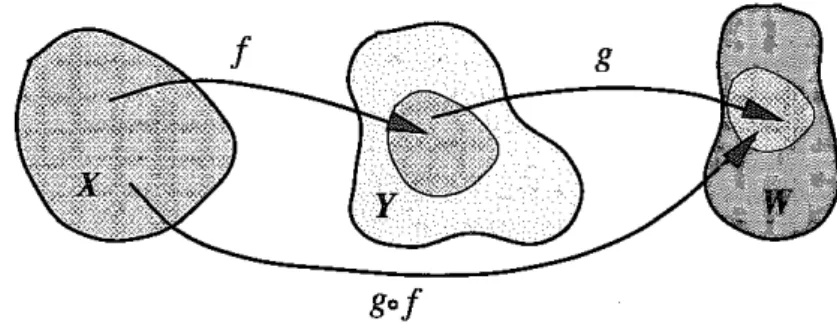
Figure 2 Thecomposition of two maps is another map.

composition oftwo maps injection, surjection, and bijection, or 1-1 correspondence inverse of a map

If

I :

X --> Y and g : Y --> W, then the mapping h : X --> W given by h(x) = g(f(x)) is' called the composition of

I

and g, and is denoted by h = g0

I

(see Figure 2).3Itis easy to verify that

loidx=l=idyol

Ifl(xI) = I(X2) implies that XI = X2,we call I injective, or one-to-one (denoted I-I). For an injective map only one element of X corresponds to an element of Y. IfI(X) = Y, the mapping is said to be surjective, oronto. A map that is both injective and surjective is said to be bijective, or to be a one-to-one correspondence. Two sets that are in one-to-one-to-one-to-one correspondence, have, by definition, the same nnmber of elements. If

I :

X --> Yis a bijection fromX ontoY, then for eachy E Y there is one and only one elementX in X for which

I(x) = y.Thus, there is a mapping I-I :Y --> X given by I-I(y) = x,where

X is the nniqne element such that I(x) = y. This mapping is called the inverse

of I.The inverse ofI is also identified as the map that satisfiesI 0 I-I = idy

and I-I 0

I

= idx-For example, one can easily verify that ln-I = exp and

exp"! = ln, becauseIn(eX

) = X andelnx = x.

Given a map

I :

X -->Y,we can define a relationtxlonX by sayingXI txl X2 if l(xI) = I(X2). The reader may check that this is in fact an equivalence relation. The equivalence classes are subsets of X all of whose elements map to the same point in Y. In fact, [x] = 1-1(f(X». Corresponding to

I,

there is a map! : X/txl--> Y given by !([x]) = I(x). This map is injective because if !([XI]) = !([X2]),then l(xI) = I(X2), so XI andX2belong to the same equivalence class; therefore, [XI] = [X2]. Itfollows that! :X/txl--> I(X) is bijective.

If

I

and g are both bijections with inverses I-I and g -I, respectively,then go

I

also has an inverse, and verifying that (g0 f)-I = I-log-I is straightforward.

0.3 METRIC SPACES 7

0.2.2. Example. As an example of the preirnage of a set, consider the sine and cosine

functions. Then it should be clearthat

. -10 {

JOO

SID = nn:n=-oo' cos-10=

{i

+

mT:

J:-oo

III

in{ectivity and surjectivity depend on the domain and

codomain

unit circle

binary operation

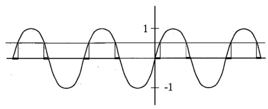
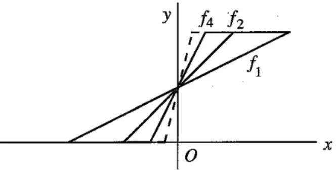
Similarly, sin- 1[O,

!l

consists ofallthe intervals on the x-axis marked

by

heavy line

segments in Figure 3, i.e., all the pointswhose sine lies between0 and~.

As examples of maps, we consider fonctions

1 :

lR-+lR stndied in calculus. The Iwo fonctions

1 :

lR -+ lR audg : lR-+ (-I,

+

I) given, respectively, by 1(x) = x3audg(x)= taubx are bijective. The latter function, by the way, shows that there are as mauy points in the whole real line as there are in the interval (-I,

+

1).Ifwe denote the set of positive real numbers by lR+, then the function 1 : lR-+ lR+ given by I(x) = x2 is surjective but not injective (bothx aud

~x map tox2 ).The function g :lR+-+ lR given by the same rule, g(x) = x2,

is injective but not surjective. Onthe other haud, h : lR+-+ lR+ again given by h(x) = x2is bijective, butu : lR-+ lR given by the same rule is neither injective

nor surjective.

LetMn x n_{denote the setofn xnreal matrices. Define a function det :M}n x n_---+

lR by det(A) = det A,where det Ais the determinaut of Afor AE J\1nxn.This fonc-tion is clearly surjective (why?) but not injective. The set of all matrices whose determinaut is 1 is det- I( I ).Such matrices occur frequently in physical

applica-tions.

Another example of interest is

1 :

C -+ lRgiven by

1

(z) = [z]. This function is also neither injective nor swjective. Here

1-

1( 1) is the unit circle, the circle of radius I in the complex plaue.

The domain of a map cau be a Cartesiau product of a set, as in

1 :

X x X -+ Y. Two specific cases are worthy of mention. The first is when Y = R An example of this case is the dot product onvectors, Thus, if X is the set of vectors in space, we cau define I(a,b) = a· b.The second case is when Y = X. Then

1

is called a binary operation on X, whereby au element in X is associated with two' elements in X. For instance, let X = Z, the set of all integers; then the fonction

I:

Z xZ-+ Zdefined by[tm, n) = mnis the binary operation of multiplication of integers. Similarly,g : lR x lR-+ lR given by g(x,y) = x

+

yis the binary operation of addition of real numbers.

0.3

Metric Spaces

Although sets are at the root of modem mathematics, they are only of formal aud abstract interest by themselves. To make sets useful, it is necessary to introduce some structnres on them. There are two general procedures for the implementa-tion of such structnres. These are the abstracimplementa-tions of the two major brauches of mathematics-algebra aud aualysis.

8 O. MATHEMATICAL PRELIMINARIES

Figure 3 The unionof all the intervals on the x-axis marked by heavyline segments is

. -1[0 1]

sm ,~ .

We canturna set into an algebraic structure by introducing a binary operation on it. For example, a vector space consists, among other things, of the binary operation of vector addition. A group is, among other things, a set together with the binary operation of "multiplication". There are many other examples of algebraic systems, and they constitute the rich subject of algebra.

When analysis, the other branch of mathematics, is abstracted using the concept of sets, it leads to topology, in which the concept of continuity plays a central role. This is also a rich subject with far-reaching implications and applications. We shall not go into any details of these two areas of mathematics. Although some algebraic systems will be discussed and the ideas of limit and continuity will be used in the sequel, this will be done in an intuitive fashion, by introducing and employing the concepts when they are needed. On the other hand, some general concepts will be introduced when they require minimum prerequisites. One of these is a metric space:

0.3.1. Definition. A metric space is a set X together with a real-valued function metric space defined d: X x X ~ lRsuch that

(a) d(x,y) 2: 0 VX,y,andd(x,y)=Oiffx=y. (b) d(x, y)= d(y, x).

(c) d(x, y) ::: d(x, z)

+

d(z, y).

(symmetry)

(the triangle inequality)

It is worthwhile to point out that X is a completely arbitrary set and needs no other structure.Inthis respect Definition 0.3.1 is very broad and encompasses many different situations, as the following examples will show. Before exantining the examples, note that the functionddefined above is the abstraction of the notion of distance: (a) says that the distance between any two points is always nonnegative and is zero ouly if the two points coincide;(b) says that the distance between two points does not change if the two points are interchanged; (c) states the known fact

0.3 METRIC SPACES 9

that the sum of the lengths of two sides of a triangle is always greater than or equal to the length of the third side. Now consider these examples:

1. Let X=

iQI,

the set of rational numbers, and defined(x,y) = Ix -

yl.

2. Let X= R, and again defined(x,y) = Ix -

yl.

3. Let X consist of the points on the surface of a sphere. We can define two distance functions on X. Letdt (P, Q) be the length of the chord joiningP and Q on the sphere. We can also define another metric, dz(P,Q), as the length of the arc of the great circle passing through points P and Qon the surface of the sphere.Itis not hard to convince oneselfthatdl and

da

satisfy all the properties of a metric function.

4. LeteO[a, b] denote the set of continuous real-valued functions on the closed interval [a, b]. We can define d(f,g) =

J:

If(x) - g(x)1 dx for f,g E

eO(a, b).

5. Leten(a, b) denote the set of bounded continuons real-valned fnnctions on the closed interval[a, b].We then define

d(f, g) = max lIf(x) - g(x)IJ

xe[a,b]

for

f,

g E eB(a, b). This notation says: Take the absolute valne of the difference in

f

andg at allxin the interval[a,b]and then pick the maximum ofall these values.

The metric function creates a natural settinginwhichtotest the "closeness" of pointsina metric space. One occasionon whichthe ideaof closeness becomes

sequence defined essential is in the study of a seqnence. A sequence is a mapping s : N--* X from the set of natural numbers N into the metric space X. Such a mapping associates with a positive integern apoints(n) of the metric space X.Itis customary to write

Sn(orXnto match the symbol X) instead ofs(n) and to enumerate the values of the function by writing{xnJ~I'

Knowledge of the behavior of a sequence for large values ofn is of fundamental importance.Inparticular, it is important to know whether a sequence approaches convergence defined a finitevalueasn increases.

0.3.2. Box. Suppose thatfor some x andfor any positive real numbere,there exists a natural number N such that dtx-; x) < e whenevern > N. Then we

say that the sequence {xn}~l converges to xandwritelimn~ood(xn lx) =

Oar d(xno x) --*0or simplyX_n--*X.

Itmay not be possible to test directly for the convergence of a given sequence because this requires a knowledge of the limit pointx. However, it is possible to

10 O. MATHEMATICAL PRELIMINARIES

Figure 4 The distance between the elements of a Cauchy sequence gets smaller and smaller.

Cauchy sequence

complete metric space

do the next best thing-to see whether the poiots of the sequence get closer and closer asn gets larger and larger. A Cauchy sequence is a sequence for which limm.n-->ood(xm, xn) = 0, as shown in Figure 4. We can test directly whether or not a sequence is Cauchy. However, the fact that a sequence is Cauchy does not guarantee that it converges. For example, let the metric space be the set of rational numbers

IQI

with the metric functiond(x,y) = Ix - YI, and consider the sequence {xn}~l where X_n = Lk~l (- li+1/k. Itis clear thatX_{n is a rational}

number for anyn. Also, to show that IX_{m -} X_n

I

4 0 is an exercise in calculus. Thus, the sequence is Cauchy. However, it is probably known to the reader that

limn--+_ooXn

=

In2,whichis nota rational number.

A metric space io which every Cauchy sequence converges is called a complete metric space. Complete metric spaces playa crucial role in modern analysis. The precediog example shows that

IQI

is not a complete metric space. However, ifthe limit poiots ofall Cauchy sequences are added to

IQI,

the resulting space becomes complete. This complete space is, of course, the real number system R Ittums out that any iocomplete metric space can be "enlarged" to a complete metric space.

0.4

Cardinality

The process of counting is a one-to-one comparison of one set with another.Iftwo cardinalily sets are io one-to-one correspondence, they are said to have the same cardinality. Two sets with the same cardinality essentially have the same "number" of elements. The setFn = {I,2, ... ,n}is finite and has cardinalityn.Any set from which there

is a bijection ontoFnis said to be finite withnelements.

Although some stepshadbeen taken before himinthe direction of a definitive theory of

sets, the creator of the theoryof sets is considered tobeGeorg Cantor(1845-1918),who

0.4 CARDINALITY 11

His father urged him to study engineering, and Cantor entered the University of Berlinin 1863 with thatintention.There he came under the influence ofWeierstrassand turned to pure mathematics. He became Privatdozent at Halle in 1869 and professorin1879. When he was twenty-nine he published his first revolutionary paper on the theory of infinite sets in theJournal fUrMathematik.Although some of its propositions were deemed faulty by the older mathematicians, its overall originality and brilliance attracted attention. He continued to publish papers on the theory of sets and on transfinitenumbers until 1897.

One of Cantor's main concerns was to differentiate among infinitesetsby"size" and, likeBalzanobefore him, he decided that one-to-one correspondence should be the basic principle. Inhis correspondencewithDedekindin1873,Cantor posed the question of whether the set of real numbers can be put into one-to-one correspondence with the integers, and some weeks later he answered in the negative. He gave two proofs. The first is more complicated than the second, which is the one most often used today.In1874 Cantor occupied himself with the equivalence of the points of a line and the points ofR"and soughtto prove that a one-to-one correspondence between these two sets was

impossible. Three years later he proved that there is such a correspondence. He wrote to Dedekind, "I seeitbut I do not believe it." He later showed that given any set, itisalways possible to create a new set, the set of subsets of the given set, whose cardinal number is larger than that of the given set.If 1'::0is the given set, then the cardinal number of the set of subsets is denoted by2~o. Cantor proved that 2~O= C,where c is the cardinal number

of the continuum; i.e., the set of real numbers.

Cantor's work, which resolved age-old problems and reversed much previous thought, could hardly be expected to receive immediate acceptance. His ideas on transfinite ordi-nal and cardiordi-nal numbers aroused the hostility of the powerful LeopoldKronecker, who attacked Cantor's theory savagely over morethana decade, repeatedly preventing Cantor from obtaining a more prominent appointment in Berlin. Though Kronecker died in 1891, his attacks left mathematicians suspicious of Cantor's work. Poincare referred to set theory as an interesting "pathological case." He also predicted that "Later generationswillregard [Cantor's]Mengenlehreas 'a disease from which one has recovered." At one time Cantor suffered a nervous breakdown, but resumed work in 1887.

Many prominent mathematicians, however, were impressed by the uses to which the new theoryhad alreadybeenpatin analysis,measuretheory,andtopology. Hilbert spreadCantor's ideas in Germany, and in 1926 said, "No one shall expel us from the paradise which Cantor created for us." He praised Cantor's transfinite arithmetic as "the most astonishing product of mathematical thought, one of the most beautiful realizations of human activity in the domain of the purely intelligible." Bertrand Russell described Cantor's work as "probably the greatest of which the age can boast." The subsequent utility of Cantor's work in formalizing mathematics-a movement largely led by Hilbert-seems at odds with Cantor's Platonic view that the greater importance of his work was in its implications for metaphysics and theology. That his work could be so seainlessly diverted from the goals intended by its creator is strong testimony to its objectivity and craftsmanship.

12 O. MATHEMATICAL PRELIMINARIES

countably infinite

uncountable sets

Cantor set constructed

Now consider the set of natnral numbers N = {l,2, 3, ... }.Ifthere exists a bijection between a set Aand N, then Ais said to be countably infinite. Some examples of countably infinite sets are the set of all integers, the set of even natnral numbers, the set of odd natnral numbers, the set of all prime numbers, and the set of energy levels of the bound states of a hydrogen atom.

Itmay seem surprising that a subset (such as the set of all even numbers) can be put into one-to-one correspondence with the full set (the set of all natural numbers); however, this is a property shared by all infinite sets. In fact, sometimes infinite sets are defined as those sets that are in one-to-one correspondence with at least one of their proper subsets.Itis also astonishing to discover that there are as many rational numbers as there are natnral numbers. After all, there are infinitely many rational numbers just in the interval (0, I)-or between any two distinct real numbers.

Sets that are neither finite nor countably infinite are said to be uncountable. In some sense they are "more infinite" than any countable set. Examples of uncount-able sets are the points in the interval(-1,

+

1),the real numbers, the points in a plane, and the points in space.Itcan be shown that these sets have the same cardinal-ity: There are as many points in three-dimensional space-the whole universe-as there are in the interval(-I,

+

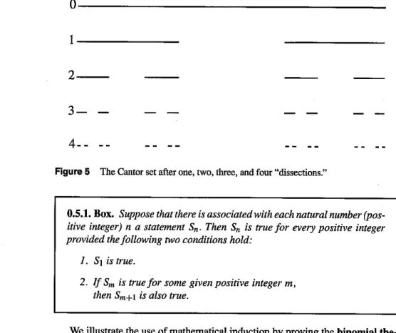
1) or in any other finite interval.

Cardinality is a very intricate mathematical notion with many surprising results. Consider the interval [0, 1]. Remove the open interval(~, ~) from its middle. This means that the points ~ and ~ will not be removed. From the remaining portion, [0, ~] U [~, 1], remove the two middle thirds; the remaining portion will then be

[0, ~]U[~, ~]U[~, ~]U[~,1]

(see Figure 5). Do this indefinitely. What is the cardinality of the remaining set, which is called the Cantor set? Intuitively we expect hardly anything to be left. We might persuade ourselves into accepting the fact that the number of points remaining is at most infinite but countable. The surprising fact is that the cardinality is that of the continuum! Thus, after removal of infinitely many middle thirds, the set that remains has as many points as the original set!

0.5

Mathematical Induction

Many a time it is desirable to make a mathematical statement that is true for all natural numbers. For example, we may want to establish a formula involving an integer parameter that will hold for all positive integers. One encounters this situa-tion when, after experimenting with the first few positive integers, one recognizes a pattern and discovers a formula, and wants to make sure that the formula holds for all natural numbers. For this purpose, one uses mathematical induction. The induction principle essence of mathematical induction is stated as follows:

(2) 0.5 MATHEMATICAL INDUCTION 13

0

1

2

-

3-

4--Figure 5 TheCantor set after one, two, three, and four "dissections."

0.5.1. Box. Suppose that there is associated with each natural number

(pos-itive integer) n a statement Sn. Then Sn is true for every pos(pos-itive integer

provided the following two conditions hold:

I. S, is true.

2. If Smis true for some given positive integerm,

then Sm+l isalsotrue.

We illustrate the use of mathematical induction by proving the binomial the-binomial theorem orem:

where we have used the notation

( ; ) '"

k!(mm~

k)!'

The mathematical statement Sm is Equation (1). We note that SI is trivially true. Now we assume that Sm is true and show that Sm+1 is also true. This means starting with Equation (1) and showing that

14 O. MATHEMATICAL PRELIMINARIES

Then the induction principle ensures that the statement (equation) holds for all

positiveintegers.

Multiply both sides of Eqnation (I) bya

+

b to obtain

(a

+b)m+l =

t

(rn)a

m- k+ l bk

+

t

(rn)a

m- kbk+1.

k~O

k

k=O

k

Now separate the k

=

0 term from the first sum and the k

=

rn

term from the

second sum:

letk=j-linthissum

The second sum in the last line involves j.Since this is a dummy index, we can substitute any symbol we please. The choicek is especially useful because then

we can unitethe two summations. This gives

Ifwe now use

which the reader can easily verify, we finally obtain

Mathematical induction is also used indefiningquantities involving integers. inductive definitions Such definitions are called inductive definitions. For example, inductive definition

is usedindefining powers: al

=

a and am

=

am-lao

0.6

Problems

tk=

n(n+ I).

k=O

2

0.6 PROBLEMS 15 0.2. Let A, B,and C be sets in a universal setU.Show that

(a) A C BandB C CimpliesA C C.

(b) AcBiffAnB=AiffAUB=B.

(c) A

c

Band B C C implies (A UB)

c

C. (d) AUB = (A ~ B) U(A

n

B)U(B ~A).

Hint: To show the equality of two sets, show that each set is a subset of the other.

0.3. For eachnE N, let

In=

I

xlix - II< n and Ix

+

II >

~}

. FindUnInandnnIn.

0.4.Show thata' E [a] implies that [a']= [a].

0.5. Can you define a binary .operatiou of "multiplication" on the set of vectors in space? What about vectors in the plane?

0.6. Show that (f ag)-1 = g-1 a1-1 when

I

and g are both bijections.

0.7. Take any two open intervals(a,b)and(c,d),and show that there are as many points in the first as there are in the second, regardless of the size of the intervals. Hint: Find a (linear) algebraic relation between points of the two intervals.

0.8. Use mathematical induction to derive the Leibnizrulefor differentiating a Leibniz rule product:

dn n (n) dk

I

dn-kg dx n(f.g) =

'E

k - dk d n-k'

k=O x x

0.9.Use mathematical induction to derive the following results:

n k rn+1 - 1

'E

r _{= ,}

k=O r - I

Additional Reading

1. Halmos, P.Naive Set Theory,Springer-Verlag, 1974. A classic text on intu-itive (as opposed to axiomatic) set theory coveriog all the topics discussed in this chapter and much more.

2. Kelley,J. General Topology,Springer-Verlag, 1985. The introductory chap-ter of this classic reference is a detailed introduction to set theory and map-pings.

3. Simmons,G.lntroduction to Topologyand Modern Analysis,Krieger, 1983. The first chapter of this book covers not only set theory and mappings, but also the Cantor set and the fact that integers are as abundant as rational

Part I

_

j

j

j

j

j

j

j

j

j

j

j

j

j

j

j

1

_

Vectors and Transformations

Two- and three-dimensional vectors-undoubtedly familiar objects to the reader-can easily be generalized to higher dimensions. Representing vectors by their

components, one can conceiveof vectors havingN components. This is themost

immediate generalization of vectors inthe plane and in space, and such vectors are called N-dimensionalCartesian vectors. Cartesian vectors are limited in two respects: Their components are real, and their dimensionality is finite. Some ap-plicationsinphysics require the removal of one or both of these limitations.Itis therefore convenient to study vectors stripped of any dimensionality or reality of components. Such properties become consequences of more fundamental defini-tions. Although we will be concentrating on finite-dimensional vector spaces in this part of the book, many of the concepts and examples introduced here apply to infinite-dimensional spaces as well.

1.1 Vector Spaces

Let us begin with the definition of an abstract (complex) vector space.'

1.1.1. Definition.A vector spaceVover <Cis a set oj objects denoted by 10), Ib), vector space defined [z),and so on, called vectors, with the following propertiesr:

1. To every pair ofvectors la) and Ib) in

V

there corresponds a vector la)

+

Ib), also in

V,

called the sum oj la) and Ib), such that

(a) la)

+

Ib) = Ib)

+

la), 1Keepinmindthat Cisthe set of complexnumbers andRthe set ofreels.

2Thebra, (I,andket,I),notation for vectors, invented by Dirac, is veryuseful whendealingwith complexvectorspaces. However,it is somewhat clumsyfor certain topicssuchas nann andmetrics andwilltherefore be abandonedinthosediscussions.