HAL Id: hal-00477695
https://hal.archives-ouvertes.fr/hal-00477695
Preprint submitted on 30 Apr 2010HAL is a multi-disciplinary open access archive for the deposit and dissemination of sci-entific research documents, whether they are pub-lished or not. The documents may come from teaching and research institutions in France or abroad, or from public or private research centers.
L’archive ouverte pluridisciplinaire HAL, est destinée au dépôt et à la diffusion de documents scientifiques de niveau recherche, publiés ou non, émanant des établissements d’enseignement et de recherche français ou étrangers, des laboratoires publics ou privés.
for travel and activity time-use pattern analysis
Tai-Yu Ma, Iragaël Joly, Charles Raux
To cite this version:
Tai-Yu Ma, Iragaël Joly, Charles Raux. A shared frailty semi-parametric markov renewal model for travel and activity time-use pattern analysis. 2010. �hal-00477695�
MA, Tai-Yu; JOLY, Iragaël ; RAUX, Charles
A SHARED FRAILTY SEMI-PARAMETRIC
MARKOV RENEWAL MODEL FOR TRAVEL
AND ACTIVITY TIME-USE PATTERN
ANALYSIS
Tai-Yu Ma
1Iragaël Joly
2Charles Raux
1 1Transport Economics Laboratory (LET), University of Lyon
2Grenoble Applied Economic Laboratory, University of Pierre Mendès France
ABSTRACT
This study investigates the influence of observed explanatory factors and unobserved random effect (heterogeneity) on episode durations of travel-activity chain. A shared frailty semiparametric proportional hazard model is proposed to estimate the transition hazard of travel/activity states. The proposed model is applied on the travel and activity episode duration analysis during evening work-to-home commute using the household travel survey data collected in the city of Lyon in France in 2005-2006. The empirical results provide useful insights for the determinants of travel and activity episode durations for evening work-to-home commute.
Keywords: time-use, activity duration, Markov renewal model, shared frailty, heterogeneity
1 INTRODUCTION
The understanding of complex travel/activity chaining behavior has been an important issue for transport system demand management and transport policy decision-making. The temporal rhythm of travel/activity chaining behavior reflects traveler’s daily mobility habit, which might be fundamental for the evaluation of transportation policy and the management of transport demand. The travel/activity chaining patterns might be influenced by many factors resulting from socio-demographic characteristics, transport supply and general urban characteristics. However, the type, timing and duration sequence visited in a travel-activity chain is basically based on individual’s schedule/reschedule process under uncertain environment. The effects of dependency between travel/activity episodes conducted in an
activity chain are often neglected. Moreover, the heterogeneity across population on the travel/activity pattern formation are general difficult to determine and hence less studied.
The widely used methods for analyzing the effects of explanatory factors on activity durations are based on hazard models (Bhat 2000). However, most studies have focused on single activity episode duration analysis. Although these studies attempt to examine the affecting factors on activity duration, they neglected the importance of dependency between travels/activities conducted in the activity chain. Recently, the effects of dependency on activity durations have been increasingly studied. Popkowski Leszczyc and Timmermans (2002) utilized conditional and unconditional parametric competing risk models to investigate the effects of sociodemographic covariates on activity duration. Their study showed that activity durations depend not only on its type but also on the duration of activity previously conducted. Joly (2006) applied duration models to analyze the stability of individual’s daily travel time. He found that individual’s activity patterns have significant effects on the daily travel time. Ma et al. (2009) applied multistate non-homogeneous semi-Markov model to estimate the influence of covariates on travel and activity duration sequence. They found significant dependency effects between adjoining travel and activity episode over individual’s travel-activity chain. For the correlation of activity type choice and its duration, Bhat (1996b) proposed a generalized multiple durations proportional hazard model to capture endogenously the influence of entrance/exit activity type choice on activity durations. Pendyala and Bhat (2004) applied discrete-continuous simultaneous equation model to investigate the casual structure of activity timing and duration. Ettema et al. (1995) applied parametric competing risk model to examine the effects of temporal constraints on activity choice, timing and its duration. The found that spatiotemporal constraints are important determinants of individual’s activity type choice, timing and durations of activities in individual’s activity chain.
Previous empirical studies showed that the heterogeneity has significant effects on activity durations, its negligence may have serious bias on duration hazard estimation (Bhat, 1996a; Klein and Moeschberger, 2003). The specification of duration hazard function should take into account this effect. To this end, a random term representing the heterogeneity may be specified into parametric/non-parametric hazards functions. The heterogeneity can be assumed following some probability distribution or unspecified and then estimated non-parametric approaches. For non-parametric heterogeneity distribution, Han and Hausman (1990) integrated a Gamma-distributed random term into the specification of hazard function. De John (1996) proposed a Weibull hazard function with a Gamma-distributed heterogeneity term to investigate the effects of covariates on individual’s vehicle holding durations. For non-parametric heterogeneity, Bhat (1996a) specified non-parametric and non-non-parametric heterogeneity into the specification of hazard function to investigate affecting effects on shopping activity durations during individual’s returning home trips after work. He found that the specification of non-parametric baseline hazard with non-parametric heterogeneity has best fit to the survey data. Differently with proportional duration hazard model, Lee and Timmermans (2007) proposed a latent class accelerated hazard model for modelling the effects of heterogeneity on activity durations. They found significant heterogeneity effects in the baseline accelerate hazard model for activity durations conducted on weekday or weekends.
MA, Tai-Yu; JOLY, Iragaël ; RAUX, Charles
The aim of the present study is twofold: firstly, to examine the effects of affecting factors on duration sequence in travel-activity chains by considering the dependency between travels/activities conducted, and secondly, to investigate the influence of unobserved random effect (heterogeneity) on the duration sequence of travel and activity chain. The formation of individual’s travel-activity duration sequence is assumed following Markov renewal process. First, the basic assumptions of Markov renewal process are discussed. Then we propose a shared frailty semiparametric model to estimate transition hazard over travel/activity episodes. The shared frailty reflecting the heterogeneity effect is assumed following Gamma distribution. We apply the proposed model for the analysis of evening after-work returning home travel-activity duration sequence in the city of Lyon. We discuss the baseline hazard of travel and activity episode durations and the influence of its determinants and the heterogeneity across household. Finally, important findings are summarized and future extensions are discussed.
2 MODEL FORMULATION
2.1 Markov renewal model
}
Consider an ordered duration sequence of travel and activity participations, called
travel-activity pattern, conducted by an individual over a period of time. The travel-activity pattern
represents the evolution of individual’s travel or activity participation over time. We assume possible activity choice is finite and identical for individuals under study. The formation of travel-activity pattern is assumed following semi-Markov process (Popkowski Leszczyc and Timmermans, 2002). The transition probability from one state to another is time-dependent, depending on affecting factors and the characteristics of its adjoining states. Let
be an observed travel-activity pattern conducted by an individual until a given censored time C, where n is the number of episodes in S. The episode represents the sojourn times of state without state transition within it. Each element in S is characterized by its travel/activity type
{
s
s
nS
=
1,...,
{
(
,
)
}
≥1=
k k k ka
t
s
Aa∈ and its entering time of episode k. A is the set of possible travel/activity choices (work, leisure, shopping, etc.). We distinguish the sequence {(ak, tk): k ≥ 0} as a Markov renewal process, and the sequence
{ }
a( )
t as a semi-Markovprocess. The schematic representation of Markov renewal process is shown in Fig. 1. We
are interested in the estimation of transition hazard in the Merkov renewal process, which represents travel/activity type-specific duration hazards with multiple entrance/exit activity type choice.
For transition hazards estimation, the survival data (travel/activity duration) is constructed for each of travel/activity episodes in individual’s travel-activity chain with competing risk (activity choice). As the transition hazard depends on its entrance and exit activity type, it is explicitly specified with respect to each pair of state transition. The duration of one episode is assumed to be a continuous random variable following some probability distribution to be estimated. Based on the assumption of semi-Markov process, the probability distribution of travel/activity durations
k k k
=
t
−
t
τ
+1 k kt
t
+1−
in episode k satisfies:)
,
T
(
P
)
,...,
,
T
(
P
t
k+1−
t
k≤
a
k+1=
j
s
1s
k=
t
k+1−
t
k≤
a
k+1=
j
s
k (1)where is a continuous random variable representing the sojourn times in the kth episode. Let represents the sojourns times in episode k since entering current state until time t. When one transition occurs, the sojourn time is evaluated with respect to the entering time of current episode k. We call the time elapsed from to t as renewal time or sojourn time with respect to episode k. The distribution of for
Τ k k t t t = − τ )( k
t
τ
k(t
)
t
k)
(t
kτ
k
=
1
,...,
n
−
1
is independent, conditional on the sequence visited by a Markov chain. The one-step transition hazard at time t (renewal time ) from state i to state j at the end of kth episode is defined as:))
(
(
kijt
k ijτ
λ
τ
kij(t
)
( )
( )
[
( )
( )
(
( )
)
( )
( )
]
h i t a j h t a h t t P t k ij k ij k ij k ij h k ij k ij = τ = + τ + τ ≤ Τ ≤ τ = τ λ → , lim 0 (2)where is the state at renewal time . The transition rate represents the changing rate of transition probability from state i to state j at renewal time . For simplification of notation, is denoted as
))
(
(
t
a
τ
kij(t
)
k ijτ
(
ijk(
t
))
k ijτ
λ
)
(t
k ijτ
) (t k ijτ
τ
hereafter. Note that at the end of one travel/activity episode, current state change to one of independent competing states. As the distribution of sojourn times at each episode is assumed independent samples conditional on the states visited previously, the estimation of transition probability can then be casted into usual competing risk hazard modeling framework. The state transition hazard visited by Markov renewal process can be estimated by counting process methods (Gill, 1980; Dabrowska et al., 1994) or classical likelihood construction methods (Kalbfleisch and Prentice, 2002). Previous empirical studies suggested that parametric models might not be appropriate for activity duration estimation since its baseline hazard is usually irregular (Bhat, 1996a). As for non-parametric hazard models, the lack of desired power in examining covariate effects on activity durations makes them less useful. The semiparametric model, namely proportional hazard model (Cox, 1972), constitutes a good candidate since it incorporates both a non-parametric baseline hazard term and a parametric function of covariates. The proportional hazard model assumes that the transition hazard is proportional to an arbitrary baseline hazard for the covariate values. As the travel-activity pattern may depend on unobserved factors resulting from individual’s variation or the influence from other members in household, the model should accommodate the unobservable random effects for transition hazard estimation. A widely used technique for modeling the heterogeneity is incorporating a random variable (frailty) in the specification of hazards function to explain unobservable common effects shared by the samples within the same group. With the shared frailty model, it provides a way to estimate the association between samples within a subgroup due to unobserved factors. As the inclusion of shared frailty in proportional hazard model needs to integrate out the frailty term of the likelihood function, the estimation of parameters is more complicated than usual proportional hazard model. The frailty term is assumed to follow some probability distributions, for which one-parameter Gamma distribution is most widely used in the literature (Duchateau and Janssen, 2008). Other probability distributions of the frailty term and detailed comparison can be found in (Hougaard, 2000). In the following, we construct the marginal likelihood function of sharedMA, Tai-Yu; JOLY, Iragaël ; RAUX, Charles
frailty term for travel-activity pattern analysis and discuss some characteristics of the shared frailty model.
Fig. 1 Schematic representation of Markov renewal process
2.2 Shared Gamma frailty semiparametric models for transition hazard
estimation
The survival data utilized for transition hazard estimation can be represented by a triplet of variables ( ), where denotes a positive random variable, representing individual m’s sojourn times in state i until the next transition to state j for episode k. represents an indicator being 1 if the transition (k, i, j) is observed for individual m, 0 otherwise. The triplet (k, i, j) denotes a transition from state i to state j at the end of kth episode. denotes the covariate column vector of (k, i, j) of individual m. The proportional hazard model assumes that the hazard of transition (k, i, j) of individual m is proportional to an unspecific baseline hazard with respect to the covariates :
k ijm k ijm k ijm
,δ
,
X
Τ
k ijmΤ
k ijmδ
k ijmX
k ijmλ
k ij 0,λ
k ijmX
(
)
( )
(
k)
ij k ijm k ij k ijm k ijm X X β ' 0 , τ exp λ = τ λ (3) where is the column vector of parameters with respect to transition (k, i, j). The above model specification assumes that all relevant covariates are incorporated to explain the variation of transition hazard. However, the unobserved effects may influence the transition hazard in the renewal process. The basic idea of shared frailty model assumes that the individuals can be divided into some subgroups where the members share common riskk ij
effects. It reflects also the association between individuals within the same subgroup sharing unobservable environment. Given a transition (k, i, j), the shared frailty has a multiplicative effect on the transition hazard. Let k
ijm
λ
denote the hazard with the frailty term for transition (k, i, j). Given an individual m of subgroup g, the transition hazard kijm
λ
with the frailty is defined by: k ijgu
(
)
( )
(
)
k ijg k ij k ijm k ij g k ijm k ijmX
u
X
β
u
' 0 ,exp
;
=
λ
τ
τ
λ
(4) where is a random variable following some probability distribution. Note that the frailty term is transition-specific, representing possible variant effects of frailty term on the transition hazards. Moreover, the hazard ratio is proportional for members within the same subgroup. Let denote the cumulative baseline hazard function with respect to the transition (k, i, j) within . For individuals in the subgroup g experiencing the transition (k,i, j), the survival function with the frailty can be constructed as:
k ijg
u
( )
∫
τλ
=
τ
Λ
0 0 , 0 ,(
)
r
dr
k ij k ij]
,
0
[
τ
k ijgu
(
)
⎥ ⎥ ⎦ ⎤ ⎢ ⎢ ⎣ ⎡ ⎟ ⎟ ⎠ ⎞ ⎜ ⎜ ⎝ ⎛ τ Λ − = τ > Τ τ > Τ = τ τ∑
∈ k ijg k ijg k ijg k ijg M m k ij k ijm k ijm k ij k ijg N N N k ij P u S ( 1,..., ) ( 1 1,..., ) exp ,0( X )expX ' β , (5)where is the set of individuals in the subgroup g experiencing the transition (k, i, j). Let denote the density function of the frailty u. The joint survival distribution can be obtained by integrating the frailty out with respect to its distribution as (Klein and Moeschberger, 2003): k ijg M
)
(u
f
U)
(u
f
U[ ]
B du u f uB Sijk Nk U ijg LP ) ( ) exp( ) ,..., ( 0 1 τ = − = τ∫
∞ (6) whereLP
[ ]
[
exp
(
)
]
is the Laplace transform of the frailty u anddef
BU
E
B
=
U−
(
k ij k ijm M m k ijm m k ij k ijg B X X ' β 0 , ( )exp∑
∈ τ Λ=
)
the sum of cumulative hazards for all individuals in the subgroup g experiencing the transition (k, i, j). The Laplace transform is very convenient for the parameter and variance estimates since its first and second derivatives can be easily obtained. As for the frailty distribution, there are three usual parametric models in the literature: (1) Gamma distribution (Clayton, 1978; Oakes 1982; Klein 1992), (2) positive stable distribution (Hougaard, 1986a) and (3) inverse Gaussian distribution (Hougaard, 1986b). As Hougaard (p246 in Hougaard 2000) argued that there is no single general distribution having all desired properties, the choice of the frailty distribution depends on the problems considered. Because we have no prior knowledge about the frailty distribution, the widely used one-parameter Gamma distribution is adopted. The advantage of one-parameter Gamma distribution resides on its computational convenience and identifiability. For the transition (k, i, j) and subgroup g, we assume the frailty is an independent and identically distributed (i.i.d.) sample from one-parameter Gamma density function of mean 1 and variance : k ijgu
k ijθ
MA, Tai-Yu; JOLY, Iragaël ; RAUX, Charles
(
)
0 ], ) / 1 ( /[ ) / exp( ) ( = 1/θ −1 − θ Γ θ θ 1/θ θk ≥ ij k ij k ij k ij k ij k ij k ij u u u f (7) where is Gamma function. As the magnitude of dependency effect may depend on its occurred episode and entrance-exit transition states (i, j), the estimation of the frailty is treated separately with respect to each transition (k, i, j). Given a transition (k, i, j), the dependence of sojourn times data with Gamma frailty in subgroup g is measured by Kendall’s withΓ
τ
τ
=
θ
/(
θ
+
2
)
(for technique details see p.138-139 in Duchateau and Janssen (2008)). Therefore, if the variance θ increases, the dependency effect becomes higher. By contrast, when the variance reduces to 0, the sojourn times data observed in one episode are independent. As the Kendall’sτ
of Gamma distribution is time-independent, the magnitude of the dependency over sojourn times is invariant.By applying the Laplace transform on the Gamma distribution, the joint survival function of Eq. (6) can be obtained as:
[
]
k ij k ijg B S N ijk k ij θ − θ + = τ τ 1/ 1,..., ) 1 ( (8)The above Gamma frailty survival function contains the parameters , and baseline hazard function to be estimated. A frequent approach for the parameters estimation is based on maximizing marginal likelihood function. The marginal likelihood with respect to transition (k, i, j) for individuals within the subgroup g can be constructed as:
k ij β k ij θ ) ( 0 , τ λk ij
[
u]
u f u du L U M m k ijg k ijm k ijg k ijm k ijm k ij k ij k ij k ijg k ijg k ijm ) ( ) exp( ) ( ) , , ( 0 0 ,∫ ∏
∞ ∈ δ Λ − τ λ = θ λ β X (9)where k is event indicator for the occurrence of transition (k, i, j) of individual m, and
ijm
δ
(
k)
ij k ijm k ijm k ij k ijm X X β ' 0 , def exp ) (τ Λ =Λ denotes individual m’s cumulative hazard without the frailty term.
As the direct maximization method is no longer applicable for semiparametric model due to the unspecific baseline hazard . Hence, we need firstly to construct likelihood function based on observed sojourn times data by considering the contribution of the frailty term. The estimates of parameters can then be iteratively achieved by Expectation-Maximization (EM) algorithm, a frequently approach for the compute of MLE with unknown parameters or missing data. Note that several alternative estimation algorithms have been proposed (Hougaard, 2000). To construct the full likelihood function, the non-parametric cumulative baseline hazard with respect to transition (k, i, j) need to be estimated. Let be the time of entering state i at kth episode for individual m and the time of entering state i of kth episode and the next transition is (k, i, j). The Nelson-Aalen estimates of cumulative baseline hazard for the transition (k, i, j) is written as:
)
(
0 ,τ
λ
k ij k im t k ijmt
∑ ∫ ∑
∈ τ ∈ δ δ = θ τ Λ k ijg k ijg M m M l k ij k ijl k il k ijm g k ij k ij dr r r u 0 ' 0 , ) exp( ) ( ) ( ) , ; ( ˆ β X X (10)where is an indicator being 1 if the transition (k, i, j) is observed for individual m within , and 0 otherwise. Similarly, is an indicator being 1 if individual l is being observed at risk within , and 0 otherwise.
)
(r
k ijmδ
)
,
[
t
t
ijmkr
k ijm+
(r) n il δ ) , [t tilk r k il +As we assume that there is no parallel activity participation at same time, the transition hazard can be estimated by considering the other competing causes as censored data. The transition hazard at the end of state i of kth episode with competing causes (travel/activities) j can be written as:
∑
∈τ
λ
=
τ
λ
k i A j k ijg k ijm k ijm g k im k im(
X
;
u
)
(
X
;
u
)
(11)where denote the set of possible exit states at the end of kth episode, depending on its current state i and occupied kth episode.
k i
A
3. ESTIMATION METHOD
To estimate the parameters of the transition hazard over episodes, we need firstly to construct the full log-likelihood function with respect to each of episodes. The MLEs of parameters and gives the maximum of log-likelihood function. Given a transition (k, i,
j), the full log-likelihood function of observed survival data , is
constructed as the partial likelihood of proportional hazard model with the frailty term (Klein and Moeschberger, 2003): k ij
β
k ijθ
)
,
,
(
ijmk k ijm k ijmδ
X
Τ
k ijM
m
∈
∀
∑ ∑
= ∈ ⎥ ⎥ ⎦ ⎤ ⎢ ⎢ ⎣ ⎡ + τ Λ − τ λ δ = θ λ G g k ijg U M m k ijm k ijm k ijg k ijm k ijm k ijg k ijm k ij k ij k ij k ij u u f u LL k ijg 1 0 , FULL , ( ,β , ) [ log( ( X )) ( X )] log ( ) (12)The full log-likelihood function can be separated into two conditional log-likelihood functions as:
)
,
(
)
(
)
,
,
(
,0 ,1 ,2 ,0 FULL , k ij k ij k ij k ij k ij k ij k ij k ij k ijLL
LL
LL
λ
β
θ
=
θ
+
λ
β
(13) with[
]
[
]
∑
∑
= = θ − − + θ + θ Γ + θ θ − = = θ G g k ij k ijg k ijg k ijg k ij k ij k ij k ij G g k ijg U k ij k ij u u N G u f LL 1 1 1 , / log ) 1 / 1 ( ) / 1 ( log log ) / 1 ( ) ( log ) ( (14) )] ( ) ; ( log [ ) , ( 1 0 , 2 , k ijm k ijm k ijg G g m M k ijg k ijm k ijm k ijm k ij k ij k ij u u LL k ijg X X − Λ τ τ λ δ = β λ∑ ∑
= ∈ (15)The first term represents the sum of logarithm of Gamma frailty distributions over all groups. The second term represents the sum of log-likelihood contribution without the frailty term. As the full log-likelihood function contains unknown parameter k, the direct estimation based
ij
θ
MA, Tai-Yu; JOLY, Iragaël ; RAUX, Charles
on Newton-Raphson method cannot be applied. A widely utilized estimation method is based on Expectation-maximization (EM) algorithm (Klein, 1992; McLachlan and Krishnan, 1997). As the EM algorithm converges very slow and needs to construct large-size observed information matrix to obtain the variance of parameters, we apply penalized partial likelihood approach (Therneau et al., 2000) for our model estimation. It has been proved that the penalized partial likelihood approach obtains exact estimates as the EM algorithm with more rapid convergence. In practice, its computational package is available with free access in R (R Development Core Team, 2005). Hence, we apply this method for our model estimation.
4. DATA DESCRIPTION
The data used in this analysis is based on household mobility surveys recently available for the city of Lyon (2006) in France with sample size of 11234 households and 27573 individuals, respectively. The questionnaire is designed to collect individual’s mobility information realized over 24 hours in the previous day for all household members of age at least 5 years. The data collected contains the mobility information in terms of origin/destination, starting/arrival time, trip purpose, transport mode etc. The daily travel and activity sequence is composed of numerous episodes of travels/activities, As the number of travel or activity episodes is large, we limit ourselves in analyzing travel-activity chain of workers conducted in the evening (after 4:00pm) after-work returning home commute.
To investigate the heterogeneity effects on transition hazards across episodes, one Cox model with Gamma-distributed frailty term is specified for each of episodes in individual’s travel-activity chain. We assume that the transition hazard is influenced by unobserved household characteristics, reflecting the interaction effects of household members and the effects from other household covariates not included in the model. Note that unobserved effects can also be estimated based on individual level to capture individual’s variation across population (Bhat et al., 2004).
For the covariate settings, previous empirical studies suggested important covariates for activity episode duration analysis (Bhat, 1996a, 1996b; Lee and Timmermans, 2007; Ma et al., 2009). Hence, individual’s socio-demographic, spatial and transport availability characteristics are taken into account. For socio-demographic characteristics, we select gender, household type, household income, employment status of two heads in the household and the number of young children less than 12 years of age in the household. For spatial and transport availability characteristics, the number of cars in household and the zonal density of household location are selected. Moreover, to investigate the effect of transportation system accessibility, two indicators are collected: distance to the nearest station of train/metro/tramway and distance to the nearest exchanger of motorway. Note that the distance is calculated as Eulerian distance from geographical zonal center to the nearest station/interchange of divided highway. The summary statistics of the covariates are listed in Table 1. As the duration of travel or activity previously conducted and the entering time of current travel/activity are important determinants of activity episode durations, these covariates are included in our model specification. The initial activity types for after-work
returning home commute are regrouped into four categories: 1. home, 2. maintenance activities (daily/weekly purchase, looking for a job, administration and health), 3. discretionary activities (walk, sports, culture and associative activities, out-of-home eating, visit to the family or to friends) and 4. other activities (Bhat and Misra, 1999). The regrouping of initial activity types is necessary in order to have enough samples to transition hazard estimation.
The final dataset contains 5627 employed individuals and 7148 trips in individual’s after-work returning home commute. The observed trips for each of purposes in evening after-work trip-activity sequence are reported in Table 2. The sample shows that 77.8 percent of workers return home directly (after 4:00pm). The other workers conduct maintenance activity (8.7%), discretionary activity (4.3%) and other (9.2%) activity for the first non-travel activity episode (EP1). As there were few individuals conducting more than one trips for after-work commute, we limit our model estimation only for the first (travel) and the second (activity) episode.
Table 1 Covariates definition and descriptive statistics
Variable Definition Mean S.E.
Socio-demographic characteristics
Gender Gender (1 if male, 0 female) 0.56 0.50
Couple 1 if couple, 0 otherwise 0.84 0.36
H_two_worker 1 if two heads of the household both have a job, 0 otherwise 0.63 0.48
H_income Household annual income: 1 under
10.000 €
, 2 = 10.000–20.000
€
, 3 = 20.001€
–30.000€
, 4 = 30.001€
–40.000€
, 5 = 40.001€
–60.000€
, 6 = more than 60.000€
3.44 1.25
N_children The number of children less than 12 years of age in household 0.66 0.92
Spatial and transport availability characteristics
N_car The number of cars available in household 1.83 0.79
Density Population density (1.000hab./km2) 4.61 6.71
Dist_I Distance to the nearest interchange of divided highway (by
100m) 40.73 43.75
Dist_P Distance to the nearest station of metro or tramway (by 100m) 27.86 26.92
Timing and duration characteristics of state/episode
Duration_EPI Duration of travel or activity conducted in previous episode (in
minute) N/A N/A
Entering_time Entering time of current state (in hours) N/A N/A
Remark: 1. Motorway is defined as a road or highway in which two directions of traffic are separated by a central barrier or strip of land without direct access (neither stops, nor traffic lights). 2. The distance is calculated as the Euclidian distance of geographical centers between zone
center and station/interchange of rail/road network.
3. The city of Lyon under study is divided into 148 zones, with median zone surface and zone density being 8.44 km2 and 16,065 habitants/km2, respectively
MA, Tai-Yu; JOLY, Iragaël ; RAUX, Charles
Table2 Number of employed individuals observed in sequential travel/activity episodes during evening work-to-home commute
Type of activity EP1 EP2 EP3 EP4
Home 4377 1003 190 33 Maintenance 488 81 12 2 Discretionary 243 58 15 2 Other 519 98 15 4 Total 5627 1240 232 41
5. ESTIMATION RESULTS
In this section, we provide Kaplan-Meier (KM) non-parametric estimator of baseline hazard for travel/activity episode durations to investigate its temporal rhythm. The travel/activity transition hazards are estimated for Cox proportional hazard models with and without Gamma frailty. The model estimation is conducted separately for each of travel/activity purposes. We present the estimation results and examine the heterogeneity effects on travel/activity duration over episodes.
5.1 Baseline hazard
As there is no prior information about parametric form of baseline hazard of activity duration, KM non-parametric method is applied. The non-parametric baseline hazard provides useful information to identify functional form for specifying parametric hazard function. It also reports temporal rhythm of activity duration. For one state transition (k, i, j), It is computed as the number of observed transition from state i to j at episode k in renewal time s divided by the number of individuals still at state i at episode k until s. The estimation method is similar as that utilized by Bhat (1996a). The KM baseline hazard functions for trip durations in the first episode are shown in Fig. 1 and Fig. 2. For home purpose, the baseline hazard shows quite irregular form with spikes at about 30-35, 45-50, 60-65, 75-80 and 90-95 minutes, indicating a general 15 minutes gaps between trips durations for returning home. For maintenance and discretionary activity participations, the baseline hazard reveals also non-monotone trends with higher stopping probability at 30-35, 45-50 and 60-65 minutes. The results suggest that parametric hazard model may not be appropriate for transition hazard estimation for trip durations. When regarding the baseline hazards for activity episode durations at EP2, it indicates a general increasing trend in baseline hazards as activity durations increases (Fig. 2). For maintenance activity, the baseline hazard shows main spikes at 5-10, 30, 50, 70 and 90 minutes. The hazard increases rapidly after 90 minutes. The results indicate that temporal rhythm for maintenance activity participations for workers during returning home commute. For discretionary activity, the baseline hazard presents a temporal pattern with spikes for each 15-minute time interval. The hazard increases rapidly
after 170 minutes. Compared with maintenance activity, the results indicate that the durations of evening after-work discretionary activity is longer and presents a larger variability.
Figure 1. Kaplan-Meier nonparametric baseline hazard for trip durations (home, first episode)
Figure 2. Kaplan-Meier nonparametric baseline hazard for trip durations (maintenance activity (left), discretionary activity (right), first episode)
MA, Tai-Yu; JOLY, Iragaël ; RAUX, Charles
Figure 3 Kaplan-Meier nonparametric baseline hazards for maintenance and discretionary activity episode durations (second episode)
5.2 Covariate effects
In this section, we examine the effects of covariates on travel/activity episode durations conducted in individual’s evening after-work commute. Note that the estimators of parameters of proportional hazard model without the frailty reflect its proportional effects on baseline hazard. The relative magnitude of the effects is measured as with and being the covariate values of individual i and j. If the heterogeneity is specified in hazard function, the hazard becomes non-proportional with respect the covariate values (Eq. (4)). To facilitate the discussion of covariate effects, we neglect the influence of heterogeneity across population in this section and discuss the effect of heterogeneity in the next section. )] ( exp[β Xi−Xj i
X
XjThe estimated effects of covariates are shown in Table 3. We discuss firstly the effects of covariates for each of travel/activity purposes in trip episode and then proceed to that of activity episodes.
The effect of gender plays a major determinant for trip durations for returning home directly after work. It reveals that women conduct longer trip durations than men. For the effect of departure time, it reveals that later the departure time is, longer is its duration. Similarly, when individuals work longer, their trip durations are longer when returning home. This might be resulted from congestion effects in the evening. Individuals reside in higher density area have shorter work-home trip durations, perhaps due to the proximity of work place and residence location. When examining covariate effects on trip durations for maintenance activity, the result reveals that women have longer trip durations for maintenance activity. It might be explained by the responsibility of household daily purchase generally assured by women. Moreover, departure time determines significantly its trip
durations for maintenance activity. It is also reasonable to find that work duration plays less influence on trip duration for maintenance activity participation. The covariate effects on trip duration for discretionary activity show quite different results than home and maintenance activity purposes. Individuals in couple households have shorter trip durations for discretionary activity participation. This indicates there may be significant interaction effects from time constraints of couple constraining individual’s destination choice in nearby work area. Individuals with one or more young children in household have shorter trip durations for discretionary activity, perhaps due to more constrained available time budget with the presence of children. Similarly, individuals with higher household income have shorter trip durations for discretionary activity participation. However, its effect is relative small compared with the influence of other covariates. On the other hand, individuals with higher vehicle availability in the household tend to travel longer. Similarly, when departure time is later, the trip duration for discretionary activity participation becomes longer. Finally, the results indicate that the accessibility at household location to transportation system has no/less significant effect on trip duration for different activity purposes.
For the second episode, it is not surprising to find that individuals with one or more children in household have shorter durations in maintenance activity participation. The results reflect the effects of available time budget for maintenance activity participation. Individuals staring maintenance activity later have longer activity durations. However, individuals travel longer to maintenance activity destination, its activity participation duration is shorter. Its effect is less important compared to that of starting time of activity and of the presence of children in household. For discretionary activity durations, the results indicate similar effects of the presence of children in household and starting time of discretionary activity as that of maintenance activity. Travel time to the destination of discretionary activity have no significant effect on its activity duration. However, individuals with higher vehicle availability have longer discretionary activity durations.
Finally, the covariates of density, accessibility to road/public transport system and household income have no significant effects on the durations of maintenance and discretionary activities during evening after-work commute.
5.3 Unobserved heterogeneity effects
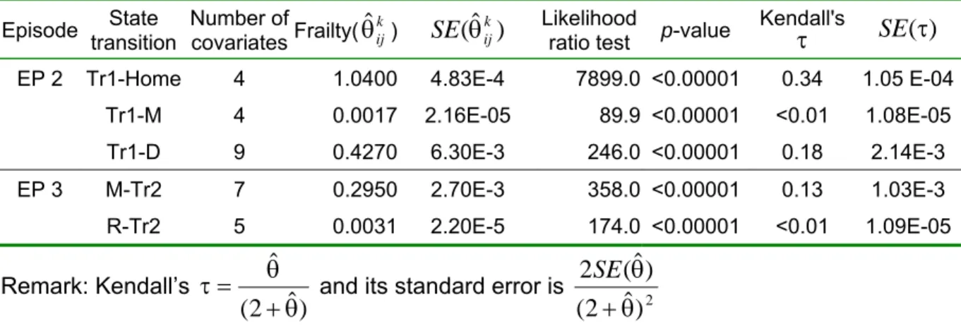
The estimators of unobserved heterogeneity based on Gamma distribution across households is reported in Table 4. The heterogeneity has multiplicative effects on baseline hazard, reflecting the interaction of travel/activity participation of household members and also unobserved effects of household characteristics on travel/activity durations. The random effect (heterogeneity) is assumed following Gamma distribution with one parametric (variance) to be estimated. We estimate one frailty model for each of travel/activity purposes over episodes. The null hypothesis of θ=0 can be based on a likelihood ratio test by
comparing estimated likelihood values of models with and without the frailty term (Andersen et al, 1996; Bhat, 1996a). Higher the estimated variance is, more significant the effects of heterogeneity on hazards across households become.
The effects of heterogeneity on transition hazards are reported for the first and second episodes. First, the likelihood ratio tests indicate that the effect of heterogeneity is
MA, Tai-Yu; JOLY, Iragaël ; RAUX, Charles ˆ ˆ =1.04 4270 . 0 ˆ = 295 . 0 ˆ = 0031 . 0 ˆ = θ
For activity episode, the effects of heterogeneity are significantly different from 0 for the duration of maintenance activity with θ . However, for discretionary activity duration, the estimated variance is close to 0 ( ) suggesting that there are few heterogeneity effects across households for this activity purpose.
Results improve our understanding of worker’s return home activity participation behaviour in how three classes of variables: sociodemographic, spatial and transport availability and timing and duration characteristics of state/episode influence trip and different activity durations. Moreover, this study identifies significant heterogeneity effects reflecting unobserved household characteristics influences on trip and activity episode durations. The results indicate that the heterogeneity effects vary over different types of activities and trips pursued in different episodes of travel and activity chains.
In this study, a shared-frailty semiparametric Markov renewal model is proposed to investigate the effects of observed and unobserved explanatory variables on travel-activity episode durations in individual’s travel-activity chains. The proposed approach provides a general framework to incorporate unobserved heterogeneity and unspecified baseline hazards in sequential activity episode duration estimations. The approach is applied to analyze trip and activity episode durations of workers’ return home trip and activity sequence in the city of Lyon, France.
6. CONCLUSIONS
The variability of the heterogeneity effects reveals that the unobserved effects on travel/activity duration depend on its activity types conducted over episodes. The negligence of this effect will bias the estimators of parameters.
statistically significant for all travel and activity episodes under study. The magnitude of estimated variance θ for trip durations of home purpose is the highest (θ ), reflecting significant heterogeneity across household level for work-home trip duration. The estimated effects of covariates with frailty term are also different from independent proportional hazard model, as shown in Table 3. The effects of heterogeneity are also significantly different from 0 for trip duration in first discretionary activity participation (θ ). However, the results indicate that there are almost no heterogeneity effects for trip duration for maintenance activity participation.
Table 3 Parameter estimates for state transition hazards over episodes with/without frailty term (t-ratios in parentheses)
State Episode
transition Model Gender Couple H_two_worker Income N_children N_car Density Dist_I Dist_P Entering_T Duration_EPI
EP 1 Tr1-H No frailty -0.1(-3.34) 0.01(4.37) -0.07(-5.52) -0.03(-34.13) Frailty -0.14(-2.99) 0.003(0.70)* -0.01(0.96)* -0.08(45.84) Tr1-M No frailty -0.21(-2.3) -0.003(-1.99) -0.26(-4.24) -0.02(-7.68) Frailty -0.21(-2.3) -0.003(-1.99) -0.26(-4.24) -0.02(-7.68) Tr1-D No frailty 0.43(1.91) -0.29(-1.69)* 0.07(2.54) 0.16(1.91) -0.39(-3.41) -0.01(-1.52)* 0.004(2.17) -0.19(-3.21) -0.01(-4.96) Frailty 0.50(1.61)* -0.24(-1.0)* 0.09(2.43) 0.20(1.7)* -0.56(-3.72) -0.03(-2.21) 0.005(2.29) -0.23(-3.00) -0.02(-5.09) EP 2 M-Tr2 No frailty 0.14(1.48)* 0.11(1.96) 0.11(1.82)* 0.002(1.45)* -0.003(-1.67)* -0.54(-9.57) 0.009(2.63) Frailty 0.19(1.64)* 0.12(1.74)* 0.14(1.75)* 0.003(1.73)* -0.004(-1.41)* -0.65(-9.77) 0.009(2.20) D-Tr2 No frailty 0.32(1.56)* 0.36(3.86) -0.23(-2.09) -0.70(-11.44) 0.007(1.65)* Frailty 0.32(1.56)* 0.36(3.86) -0.23(-2.09) -0.70(-11.44) 0.007(1.65)*
Remark: 1.H: home, M: maintenance activity, D: discretionary activity 2. p-values are reported only for significance at 0.05 level except *
MA, Tai-Yu; JOLY, Iragaël ; RAUX, Charles
Table 4 Model fit statistics for proportional hazard model with Gamma frailty (heterogeneity)
Episode transition State Number of covariates Frailty( k)
ij
θˆ
SE
(
θ
ˆ
ijk)
Likelihood ratio test p-value Kendall'sτ
SE
(τ
)
EP 2 Tr1-Home 4 1.0400 4.83E-4 7899.0 <0.00001 0.34 1.05 E-04
Tr1-M 4 0.0017 2.16E-05 89.9 <0.00001 <0.01 1.08E-05 Tr1-D 9 0.4270 6.30E-3 246.0 <0.00001 0.18 2.14E-3 EP 3 M-Tr2 7 0.2950 2.70E-3 358.0 <0.00001 0.13 1.03E-3 R-Tr2 5 0.0031 2.20E-5 174.0 <0.00001 <0.01 1.09E-05 Remark: Kendall’s
)
ˆ
2
(
ˆ
θ
+
θ
=
τ
and its standard error is2
)
ˆ
2
(
)
ˆ
(
2
θ
+
θ
SE
ACKNOWLEDGEMENTS
This research has benefited from a grant of ANR (the French Agency for Research), Project EuroCities-DATTA n° ANR-07-BLAN-0032-01
REFERENCES
1. Andersen, P. K., Borgan, O., Gill, R. D., Keiding, N. (1996) Statistical Models Based on Counting Processes (Springer Series in Statistics), corrected Edition. Springer.
2. Bhat, C.R. (1996a). A hazard-based duration model of shopping activity with nonparametric baseline specification and nonparametric control for unobserved heterogeneity. Transportation Research Part B 30(3), 189–207.
3. Bhat, C.R. (1996b) A generalized multiple durations proportional hazard model with an application to activity behavior during the evening work-to-home commute. Transportation Research Part B 30(6), 465–480.
4. Bhat, C.R., Misra, R. (1999). Discretionary activity time allocation of individuals between in-home and out-of-home and between weekdays and weekends. Transportation 26 (2), 193–209.
5. Bhat, C.R. (2000). Duration Modeling. In Handbook of Transport Modelling, (D.A. Hensher and K.J. Button, eds), Elsevier Science, pp. 91-111.
6. Bhat, C.R., Frusti, T., Zhao, H., Schönfelder, S., Axhausen, K.W. (2004) Intershopping duration: an analysis using multiweek data. Transportation research Part B 38, 39-60. 7. Clayton, D.G. (1978). A model for association in bivariate life tables and its application in
epidemiological studies of familial tendency in chronic disease incidence. Biometrika 65, 145–151.
8. Cox, D. R. (1972). Regression Models and Life Tables. Journal of the Royal Statistical Society B 34, 187-200.
9. Dabrowska, D.M., Sun, G.W., Horowitz, M.M. (1994). Cox regression in a Markov renewal model: an application to the analysis of bone marrow transplant data. Journal of
the American Statistical Association 89(427), 867–877.
10. De Jong, G.C., (1996) A disaggregate model system of vehicle holding duration, type choice and use. Transportation Research Part B 30(4), 263–276.
11. Duchateau, L., Janssen, P. (2008). The Frailty Model. Springer-Verlag New York.
12. Ettema, D., Borgers, A., Timmermans, H.J.P. (1995). Competing risk hazard model of activity choice, timing, sequencing, and duration. In: Transportation Research Record: Journal of the Transportation Research Board. No. 1493. Transportation Research Board of the National Academies. Washington. D.C., 101–109.
13. Gill, R.D. (1980). Nonparametric estimation based on censored observations of a Markov renewal process. Probability Theory and Related Fields 53(1), 97-116.
14. Han, A., Hausman, J.A., (1990) Flexible parametric estimation of duration and competing risk models. Journal of Applied Econometrics 5, 1–28.
15. Hougaard (1986a) A class of multivariate failure time distributions. Biometrika 73, 671-678.
16. Hougaard (1986b) Survival models for heterogeneous populations derived from stable distributions. Biometrika 73, 387-396.
17. Hougaard, P. (2000). Analysis of Multivariate Survival Data. Springer-Verlag New York. 18. Joly I. (2006). Test of the Daily-Travel-Time stability using a duration model. International
Journal of Transport Economics, Vol. XXXIII, n°3, p. 369-400
19. Kalbfleisch, J.D., Prentice, R.L. (2002). The Statistical Analysis of Failure Time Data. New York: John Wiley & Sons. Inc. 2nd Edition.
20. Klein, J.P., (1992). Semiparametric estimation of random effects using the Cox model based on the EM algorithm. Biometrics, 48, 795–806.
21. Klein, J.P., Moeschberger, M.L. (2003). Survival analysis–techniques for censored and truncated data.Springer, New York (2nd ed.).
22. Lee, B., Timmermans, H.J.P. (2007). A latent class accelerated hazard model of activity episode durations. Transportation Research Part B 41(4), 426-447.
23. Ma, T.Y., Raux, C., Cornelis, E., Joly, I. (2009). Multi-state non-homogeneous semi-markov model of daily activity type, timing and duration sequence. Transportation Research Record: Journal of the Transportation Research Board, No. 2134, 123-134. 24. McLachlan, G.J., Krishnan, T. (1997). The EM Algorithm and Extensions. John Wiley &
Sons, New York.
25. Oakes, D. (1982). A model for association in bivariate survival data. Journal of the Royal Statistical Society series B 44, 414–422.
26. Pendyala, R.M., Bhat, C.R. (2004). An exploration of the relationship between timing and duration of maintenance activities. Transportation 31, 429–456.
27. Popkowski Leszczyc. P.T.L., Timmermans, H. (2002). Unconditional and conditional competing risk models of activity duration and activity sequencing decisions: An empirical comparison. Journal of Geographical Systems 4, 157–170.
28. R Development Core Team. (2005). R: A language and environment for statistical computing. R Foundation for Statistical Computing, Vienna, Austria. ISBN 3-900051-07-0, URL: http://www.R-project.org.
29. Therneau, T.M., Grambsch, P.M., Pankratz, V.S. (2000). Penalized survival models and frailty. Technical Report #66, Mayo Foundation.