Publisher’s version / Version de l'éditeur:
ASHRAE Transactions, 92, 1A, pp. 103-115, 1986
READ THESE TERMS AND CONDITIONS CAREFULLY BEFORE USING THIS WEBSITE. https://nrc-publications.canada.ca/eng/copyright
Vous avez des questions? Nous pouvons vous aider. Pour communiquer directement avec un auteur, consultez la première page de la revue dans laquelle son article a été publié afin de trouver ses coordonnées. Si vous n’arrivez pas à les repérer, communiquez avec nous à [email protected].
Questions? Contact the NRC Publications Archive team at
[email protected]. If you wish to email the authors directly, please see the first page of the publication for their contact information.
NRC Publications Archive
Archives des publications du CNRC
This publication could be one of several versions: author’s original, accepted manuscript or the publisher’s version. / La version de cette publication peut être l’une des suivantes : la version prépublication de l’auteur, la version acceptée du manuscrit ou la version de l’éditeur.
Access and use of this website and the material on it are subject to the Terms and Conditions set forth at
The utilization of internal heat gains
Barakat, S. A.; Sander, D. M.
https://publications-cnrc.canada.ca/fra/droits
L’accès à ce site Web et l’utilisation de son contenu sont assujettis aux conditions présentées dans le site LISEZ CES CONDITIONS ATTENTIVEMENT AVANT D’UTILISER CE SITE WEB.
NRC Publications Record / Notice d'Archives des publications de CNRC:
https://nrc-publications.canada.ca/eng/view/object/?id=ddbb44e3-8eb4-425d-9df9-4b9656914a32 https://publications-cnrc.canada.ca/fra/voir/objet/?id=ddbb44e3-8eb4-425d-9df9-4b9656914a32Ser
TH1 - --
N21d
National
Research
Con$eil national
no.
1452
I*
Council Canada
de recherche=
Canada
Institute for
Research in
Construction
lnstitut de
recherche en
construction
The Utilization of Internal Heat Gains
by S.A. Barakat and D.M. Sander
Reprinted from
ASHRAE Transactions 1986
Vol. 92, Pt. 1A, p. 103-115
(IRC Paper No. 1452)
Price $3.00
NRCC 27637
I
NRC
-
C mOn a d e d u i t l e s f a c t e u r s d ' u t i l i s a t i o n d e s g a i n s thermiques i n t e r n e s
3
p a r t i r d'une s i m u l a t i o n h e u r e p a r h e u r e s u r o r d i n a t e u r b a s s e s u r l e s donnges m6t6orologiques r g e l l e s c o n c e r n a n t 11 e n d r o i t s a u Canada. Ces f a c t e u r s d ' u t i l i s a t i o n s o n t exprimgs e n f o n c t i o n du r a p p o r t e n t r e l e t o t a l d e s g a i n s i n t e r n e s s a i s o n n i e r s e t l a p e r t e d e r g f g r e n c e t o t a l e p a r s a i s o n pour t r o i s p r o f i l s q u o t i d i e n s d e g a i n s i n t e r n e s e t q u a t r e n i v e a u x d e s t o c k a g e thermique. On p r s s e n t e d e s courbes r e p r g s e n t a n t l a t e m p s r a t u r e i n t s r i e u r e c o n s t a n t e e t d e s 6 1 6 v a t i o n s d e t e m p e r a t u r e a d m i s s i b l e s d e 2,75 et 5,5OC. Pour l e s maisons d o n t l e r a p p o r t e n t r e les g a i n s i n t e r n e s e t l a p e r t e thermique d e r g f 6 r e n c e est i n f s r i e u r 3 0,4, a n p e u t u t i l i s e r t o u s l e a g a i n s i n t e r n e s pour compenser les p e r t e s thermiques. De p l u s , onse
s e r t a u s s i d e l a mgthode d e s f a c t e u r s d ' u t i l i s a t i o n pour c a l c u l e r l e s b e s o i n s e n c h a u f f a g e d ' a u t r e s b 3 t i m e n t s,
p a r exemple l e s immeubles3
a p p a r t e m e n t s , l e s 6 c o l e s e tl e s
immeubles3
bureaux.No. 2940
THE UTILIZATION OF INTERNAL HEAT GAINS
S.A.
Barakat, Ph.D., RE.D.M.
Sander,P.E.
ABSTRACT
Utilization factors for internal heat gains have been derived from an hour-by-hour computer simulation using actual weather data for 11 Canadian locations. These utilization factors are expressed as a function of the ratio of seasonal total internal gains to seasonal total
reference loss for three daily profiles of internal gains and four levels of thermal storage. Curves are presented for conditions of constant room temperature and for allowable temperature rises of 2.75 and 5.5OC. For houses with a ratio of internal gains to reference heat loss of less than 0.4, all internal gains can be utilized to offset thermal losses. In addition, the application of the utilization factor method is extended to calculation of heating energy requirements of other buildings such as apartments, schools, and offices.
INTRODUCTION
Calculation of the energy to heat a building requires a means of accounting for all thermal losses and gains. One proposed method was based on a simple heat balance and a solar
utilization factor expressed as a function of building heating load, solar gain, and thermal mass of the building (Sander and Barakat 1983). This method was applied graphically on a seasonal basis (Barakat and Sander 1982) and in a computer program as a monthly calculation (Dumont et al. 1982).
Determination of heating load requires evaluation of internal gains. The magnitude of such gains, due to people, appliances, lights, and hot water, may be estimated from occupant use data. For normal houses the authors suggested that all these internal gains can be utilized to offset seasonal heating requirements. The previous studies are extended to investigating the utilization of internal gains in a manner similar to that for solar gains and determining a utilization factor to account for the loss characteristics of the building, the thermal mass, the temperature swing allowed, and the time profile, as well as the
magnitude of the internal gains.
The results confirm the assumption that virtually all internal gains are usable for "normal" houses in which seasonal internal gains are less than 25% of the seasonal heat loss. In addition, the calculation method is extended to cases in which this is not true, for example, superinsulated houses or small buildings of nonresidential occupancy that have relatively large internal gains. A more accurate monthly calculation, especially for the spring and fall months, also becomes possible.
UTILIZATION FACTOR CONCEPT
The concept of a uttlization factor to account for the usable portion of internal and solar gains is summarized below (Sander and Barakat 1983).
S.A. Barakat and D.M. Sander, Building Services Section, Division of Building Research, National Research Council of Canada, Ottawa, Canada, KIA OR6.
Instantaneous Heat Balance
The instantaneous (hourly) heat balance is given by:
where h = instantaneous heating required,
It
= instantaneous heat loss due to transmission through exterior walls, windows, ceilings, etc.,1, = instantaneous heat loss due to air exchange with outdoors (infiltration plus ventilation),
lb = instantaneous below-grade heat loss,
gi = instantaneous heat gain from internal sources (lights, equipment, people, etc. ), gs = instantaneous solar heat gain through windows.
When gains exceed losses, the excess heat is stored in the mass of the room and the room temperature rises. To prevent the room temperature from rising above an acceptable limit, the excess heat must be removed by opening windows or by operating a ventilation or
air-conditioning system. A portion of the stored heat becomes available when the room
temperature drops to the thermostat setting. The remainder will have been lost in the form of increased transmission losses due to rise in room temperature.
Seasonal Heat Balan~ce
The heat balance equation may be written for a longer time period, a month or a season, by including utilization factors to account for the usable portion of internal and solar gains, that is,
where H = total heating required for season,
Lt = seasonal total of heat losses due to transmission through exterior walls, windows, ceilings, etc.
La = seasonal total of heat losses due to indoor-outdoor air exchange (infiltration plus ventilation),
Lb = seasonal total below-grade heat loss,
GI = seasonal total of heat gains from internal sources lights, equipment, people, etc.),
Gs = seasonal total of solar heat gains through windows, qi = utilization factor for internal gains,
qs = utilization factor for solar gains. Utilization Factor for Solar Gain
The solar utilization factor, qs, was correlated to two normalized parameters, one of which is the gain-load ratio (GLR) defined as
GLR = Gs/Qn ( 3 )
The net heating load, Qn, is the amount of heating energy required, in the absence of solar gains, to maintain room temperature at the heating thermostat setting, or
The determination of Q,,, therefore, requires an estimate of the utilization factor for internal gains, qi.
Utilization Factor for Internal Gain
The fraction of internal gains that are useful in offsetting heat losses depends upon the magnitude of the internal gains, the profile or variation of these gains with time, the heat losses, the thermal storage characteristics of the building, and the temperature rise that is allowed before excess heat is dumped.
In the same manner as for the solar utilization factor, the internal gain utilization factor can be expressed as a function of two normalized parameters, the internal gain-loss
ratio (IGLR) and the mass-internal gain ratio (MIGR). The internal gain-loss ratio is defined as the ratio of the internal gains to the building heat loss (calculated at the thermostat setting)
IGLR = Gi
Lt
+
La+
L,,For Canada, a house built to pre-1975 standards would typically have an IGLR of less than 0.1; a superinsulated house would have an IGLR of 0.3 to 0.4.
The mass-internal gain ratio is defined as the ratio of the thermal capacity of the building interior, C, (MJ/K) to the average hourly internal gain over the season, gi, (MJ/h), that is
C
MIGR =
-
(h/K)gi
Thermal capacity, C, is the effective mass of the building multiplied by its specific heat. A guide to thermal capacity values is given in Table I. Typical houses of lightweight construction have a MIGR of approximately 1.5 h/K.
DEVELOPMENT OF INTERNAL GAIN UTILIZATION FACTORS
Utilization factors for internal gain were obtained from a large number of computer
simulations. The computer program performs hour-by-hour calculations to determine heat gains and losses, the heating energy required to maintain room temperature, and the temperature rise due to excess gains.
Thermal storage effects were simulated using the ASHRAE thermal response method (ASHRAE 1981). Thermal response factors used were for light, medium, heavy, and very heavy
construction (Sander and Barakat 1983).
A heating thermostat setting of 21°C was assumed. As occupant preference would determine the allowable rise in room temperature, three different cases were considered: a constant room temperature, and allowable rises of 2.75OC and 5.5OC. It was assumed that the room temperature was prevented from rising above the allowable limit by ventilating with outside air.
The simulation was carried out for 11 locations representing the climatic regions of Canada (Vancouver, Summerland, Edmonton, Swift Current, Winnipeg, Windsor, Toronto, Ottawa, Montreal, Frederiction, and Goose Bay). A full year of measured weather data, chosen to be
"typical," were used for each location. Building Models
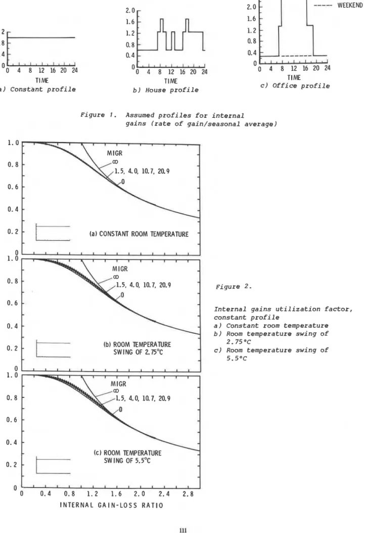
Three profiles of internal gain were considered: a constant gain, a typical house profile with peaks in the morning and evening, and a typical office profile with large gains during normal working hours. The assumed profiles are shown in Figure 1.
Twenty variations of building heat loss characteristic were chosen so as to give a wide range of internal gain to loss ratio. The heating season for all locations was taken as October to April, inclusive. Seasonal values for the internal gain utilization factor, qi, the IGLR, and the MIGR were determined for this period. A curve-fitting routine was then used to obtain the best curve fit of qi as a function of the IGLR for each of the light, medium, heavy, and very heavy constructions; these correspond to values of MIGR equal to 1.5, 4.0,
10.7, and 20.9, respectively. The curves are shown in Figures 2, 3, and 4 for the three profiles considered. Each figure shows a set of three graphs (a to c) corresponding to the
I allowable temperature swing of 0, 2.75 and 5.5OC, respectively. In addition to the curves for
the four values of MIGR, each graph also shows the limiting cases of no thermal storage
(instantaneous response) and infinite thermal storage. Examples of the calculated data points and corresponding curve fits are given in Appendix A.
DISCUSSION
Figures 2 and 3 reveal that for the constant and house internal gain profiles the effect of thermal storage on the utilization of internal gains is very small, and in some cases negligible. This is due to the even distribution of the gains through the day and from day-to-day
, reducing the need for thermal storage to carry over excess gains to the
nighttime or cloudy days, as is the case for solar gains. Consequently, for these profiles a single curve fit can be produced for points representing all four mass levels. These curves are shown in Figures 5 and 6 for the constant and house profiles, respectively. It is
apparent from Figures 5 and 6 that the increase in internal gain utilization as a result of a larger temperature swing is quite limited. In fact, for the house profile, there is no increase in
ni due to increasing temperature swing above 2.75, while for the constant profile
there is negligible improvement with increased allowable temperature swing.Figures 5 and 6 also indicate that for most houses (IGLR up to 0.4) with a constant or house internal gain profile, the seasonal utilization factor is very close to 1.0. For higher IGLR or for buildings with an office profile (small office buildings, schools, etc.), the utilization factor can be obtained from Figure 3 or from the correlation equations given in Appendix A.
In most cases, when calculating the energy consumption of a house the daily profile of internal gains is not well defined, nor is the temperature swing or mass level. For both house and constant profiles the values of qi were very similar for all mass levels and allowable temperature swings considered.
A further simplification, therefore, is to reduce all utilization factors presented in Figures 5 and 6 to a single correlation curve. A curve fit for all data points produced the equation
with an rms error of 0.018. Equation 7 applies for 0
<
IGLR < 2.2. For IGLR>
2.2, qi reaches the limiting case of "infinite storage" and can be calculated asUse and Limitations
The procedure described by Sander and Barakat (1983), and used in conjunction with the internal gain utilization factor curves and equations presented here, provides a simple method of estimating the heating energy requirement of houses and small buildings with an
officelike occupancy. The general procedure is summarized as follows:
-
calculate the loss and gain components Lt, La, Lb, Gi, and Gs,-
calculate IGLR from Equation 5,-
calculate MIGR (note: this is of no consequence unless the profile is for office),-
obtain qi, corresponding to IGLR and MIGR for the desired allowable temperature rise, from the appropriate Figure (4 to 6); for a house, Equations 7 and 8 may be used instead of the figures,
-
substitute qi into Equation 4 to obtain the net heating load,a,
-
use the procedure introduced by Sander and Barakat (1983) to obtain the solar gain utilization factor, qs,-
obtain the heating requirement from Equation 2.The basic assumption of this heat balance approach is that all heat gain and loss
components are additive. This implies a well-mixed or single-zone type of thermodynamic model in which temperature is uniform throughout and heat gains offset heat losses. This is
generally a valid assumption for houses that have a relatively open plan or forced air circulation. Larger buildings or those in which the spaces are thermally separated may be treated as the sum of separate zones, where each zone is calculated using the above procedure, provided that interzone heat transfer can be neglected. This approach has been widely used with energy analysis programs, such as the ESA series (ESA n.d.), that perform a single-zone thermal simulation.
It should be noted that the accuracy of the heating energy estimate is more dependent on the calculation of heat losses and gains than on the utilization factors themselves. The heat loss and gain calculations must allow for factors such as lowering of the thermostat setting at night, correct estimation of a seasonal average air-change rate, and the proper estimate of internal gains from various sources. Generally, the uncertainty associated with calculating losses and gains is much larger than that associated with the utilization factors.
SUMMARY AND CONCLUSION
Utilization factors for internal gains were derived using an hour-by-hour computer simulation with actual weather data for 11 Canadian locations. These utilization factors are expressed as a function of the ratio of seasonal total internal gains to seasonal total reference loss for three daily profiles of internal gain and four levels of thermal storage. Curves are presented for conditions of constant room temperature and for allowable temperature rises of 2.75 and 5.5OC.
The following conclusions can be drawn:
1. For houses with a ratio of internal gains to reference heat loss of less than 0.4, all internal gains can be utilized to offset thermal losses.
2. For buildings with a "constant" or a "house" internal gain profile, increasing the thermal storage mass or the allowable temperature swing has a negligible effect on the utilizatioaof internal gains.
3. For practical purposes, the following equation can be used to calculate the seasonal internal gain utilization factor for houses:
1.0
+
0.054 IGLR~.'~"
= 1.0+
0.24 IGLR 3.06 for IGLR<
2.2, and for IGLR>
2.2. 1 ni =-
IGLR4. The simple method of calculating heating energy requirements, based on a monthly or seasonal heat balance equation and utilization factors for solar and internal heat gains (previously limited to houses), can be applied to other buildings such as apartments, schools, offices, etc., by using the utilization factors given by Figure 3.
REFERENCES
ASHRAE. 1981. ASHRAE Handbook
-
1981 fundamentals, Chapter 28. Atlanta: American Society of Heating, Refrigerating and Air Conditioning Engineers.Barakat, S.A., and Sander, D.M. 1982. "A method for optimizing south window area of houses." Proceedings of ASHRAEIDOE Conference on Thermal Performnace of Building Envelopes, Dec. Dumont, R.S.; Lux, M.E.; and Orr, H.W. 1982. "HOTCAN: A computer program for estimating the
space heating requirement of residences." National Research Council of Canada, Division of Building Research, CP 49.
ESA. n.d. Energy systems analysis series of programs. Ross. F. Meriwether Associates,, San Antonio, Texas.
Sander, D.M., and Barakat, S.A. 1983. "A method for estimating the utilization of solar gains through windows." ASHRAE Transactions, Vol. 89, Part lA, p. 12-22.
TABLE 1
Thermal Capacities of Buildings - - - - -
Thermal Capacity
M J / K - ~ ~ floor area Description
Standard frame construction, 12.7- gyproc walls and ceilings, carpet over wooden floor (light*)
0.15 As above, but 50.8- gyproc walls and 25.4- gyproc ceiling (medium*)
0.41 Interior wall finish of 101.6-mm brick, 12.7- gyproc ceiling, carpet over wooden floor (heavy*)
0.20 Commercial building, 76-m concrete floor
-- -
0.31 Commercial building, 1 0 2 - n ~ ~ concrete floor
0.45 Commercial building, 152- concrete floor
0.81 Very heavy commerial building, 305- concrete floor (very heavy*) *Constructions referred to in text.
APPENDIX A Simulation Results Seasonal Internal Gain Utilization
A total of 4 5 seasonal utilization factor curves were produced (3 profiles, 3 allowable temperature rises, and 5 thermal storage levels). For values of IOLR less than 2.2, the data points may be represented by a well-defined correlation curve of the form,
(A. 1) Examples of data and corresonding curve fits are illustrated in Figure Al. Values of the cor~elation parameters al, a a3, and a4 are given along with the value qf the root mean square (rms) error in Table
a;.
As indicated in the text, all cases for house and constant profiles can be represented by one correlation, A single set: of pariimeters is, therefore, given for these profiles.Mo,n&hly Internal Ga$n Utilization
Energy caloulations are often performed on a monthly rather than a seasonal basis. The values of the internal gain utilization factor and the internal gain-loss ratio for each month of the heating season for all lscations were calculated. Monthly data points for the same cases shown in Figure A1 are then reproduced on a monthly basis in Figure A2 together with their corresponding curve fit, A single curve fit is used for all house and constant profile dqta points. The correlation constants for each curve fit are given in Table A-2. The fittipg equation has the following form:
for IGLR
<
lower limit,for lower limit
<
IGLR<
upper limitto IGLR upper limit
TABLE A1
Correlation Constants for Seasonal Data Points*
Profile Temp. Mass rms
Swing, OC Level
a
1 a2 a3 a4 errorOffice 0 L M H VH 2.75 L M H VH 5.5 L M H VH House and A1 1 All Constant I + ~,(IGLR)~~
*
"1-
0<
IGLR 6 2.2 1+
E ~ ~ ( I G L R ) ~ ~TABLE A2
Correlation Constants for Monthly Data Points
Temp. IGLR Limit
Swing, Mass rms
Profile OC Level P1 P2 3 Error Lower Upper
Office 0 L 0.082 1.096 -0.174 0.027 0.3 5.5 M 0.076 1.336 -0.018 0.025 0.3 5.5 H 0.175 1.400 0.109 0.021 0.3 5.0 VH 0.275 1.539 0.314 0.019 0.3 5.0 2.75 L 0.204 1.336 0.115 0.027 0.3 5.0 M 0.222 2.309 0.657 0.023 0.3 5.0 H 0.518 2.557 1.734 0.019 0.7 5.0 VH 0.735 2.200 2.836 0.019 0.7 5.0 5.5 L 0.194 1.921 0.465 0.027 0.3 5.0 M 0.453 1.849 0.812 0.025 0.3 5.0 H 0.709 2.045 2.563 0.022 0.7 5.0 VH 0.788 2.053 3.122 0.021 0.7 5.0 House
and All All 0.675 2.358 2.342 0.029 0.7 5.0
0 -0 4 8 12 16 2-0 24 TI ME a ) Constant profile
A
'0 4 8 12 16 20 24 TlME b ) House profile 2.8:;ii[[
WEEKDAY WEEKEND1.2 0.8 0.4
---
0 0 4 8 12 16 20 24 TlME C ) Office profileFigure I. Assumed profiles for internal
gains (rate of gain/seasonal average)
0 0 0 . 4 0 . 8 1 . 2 1 . 6 2 . 0 2 . 4 2 . 8 I N T E R N A L G A I N - L O S S R A T I O 1.5. 4.0, 10.7, 20.9 .5, 4.0. 10.7, 20.9 (b) ROOM TEMPERATURE SWING OF 2.75"C .5, 4.0, 10.7. 20.9 (c) ROOM TEMPERATURE SW ING OF 5.5"C Figure 2.
Internal gains utilization factor, constant profile
a ) Constant room temperature b ) Room temperature swing of
2.75 OC
C ) Room temperature swing of 5.5OC
3 ' c l
g x
;
$ 8
+ P 3S W
'tl P, C ( kg
'3k %
'
'
@ I * . 3-
*
z
= Y I*. 7 OI k 0 I * V)1 v '
N tt !-.g
b
0 3i
Ch 0 . N P,%
a 0 cl N ?I I*.'2
'-4 ID IPI c m I*. k I*. N P, t-t I*.S
U T I L I Z A T I O N F A C T O R U T I L I Z A T I O N F A C T O RI N T E R N A L G A I N - L O S S R A T I O
F i g u r e 5 . I n t e r n a l g a i n u t i l i z a t i o n f a c t o r , c o n s t a n t p r o f i l e , a l l mass l e v e l s
I N T E R N A L G A I N - L O S S R A T I O
U T I L I Z A T I O N F A C T O R *'a 0 I D 0
*
3 r.*
D 3 ID w h l c D D * + rC r.-
P.
C O P . P P P P .r o N n u. w 0 0 N P u. w o U T l L l Z A T l O N F A C T O RDiscussion
G.
WILL, G.K. Yuill & Assoc., Ltd, Winnipeg, Canada: I have carried out similar modeling, using a radiation balance in each room. I found that the internal gain utilization factor never reaches 1.0, because radiation raises the wall temperature, and thus the losses. Did you consider this effect in your analysis? Do you believe that the utilization factor would ever reach 1.0 in a real house?BARAKAT: The ASHRAE response factor method, used to produce the utilization factors, assumes that all energy transferred into the space eventually appears as space cooling load. As Dr. Yuill mentioned, this is not exactly true. The radiant component of the gain raises the wall temperature leading to some losses to the surroundings. This can be
approximately corrected for using the method described in the Handbook (Chapter 26, Eq. 36, 1985).
Because the correction applies to the radiant component of the gain only, it is expected to have a small effect on the utilization factor, particularly for well insulated buildings. It is, therefore, expected that the utilization factor for internal gains will be between 0.95 and 1.0 for small values of JGLR. The errors in energy calculations due to the uncertainty in this value are much less than those due to the uncertainty in the estimated values of the internal heat gain from various sources.
T h i s paper i s being d i s t r i b u t e d i n r e p r i n t form by t h e I n s t i t u t e f o r Research i n Construction, A l i s t of b u i l d i n g p r a c t i c e and r e s e a r c h p u b l i c a t i o n s a v a i l a b l e from t h e I n s t i t u t e may be obtained by w r i t i n g t o t h e P u b l i c a t i o n s S e c t i o n , I n s t i t u t e
f o r
Research i n Construction, N a t i o n a l Research C o u n c i l of Canada, O t t a w a , O n t a r i o ,
KIA
OR6.Ce document e s t d i s t r i b u g sous forme de t i r e - a - p a r t p a r l l I n s t i t u t de recherche e n c o n s t r u c t i o n . On peut o b t e n i r une l i s t e d e s p u b l i c a t i o n s de 1 ' I n s t i t u t p o r t a n t s u r les techniques ou l e s recherches en matigre de batiment en 6 c r i v a n t