Cochlear tuning… of mice and men

Cochlear tuning… of mice and men

The MIT Faculty has made this article openly available.

Please share

how this access benefits you. Your story matters.

Citation

Farrahi, Shirin, Ghaffari, Roozbeh, Sellon, Jonathan Blake,

Nakajima, Hideko H. and Freeman, Dennis M. 2018. "Cochlear

tuning… of mice and men." AIP Conference Proceedings, 1965 (1).

As Published

http://dx.doi.org/10.1063/1.5038463

Publisher

Author(s)

Version

Author's final manuscript

Citable link

https://hdl.handle.net/1721.1/122671

Terms of Use

Creative Commons Attribution-Noncommercial-Share Alike

Cochlear Tuning... of Mice and Men

Shirin Farrahi

, Roozbeh Ghaffari

, Jonathan B. Sellon

, Hideko H. Nakajima

and Dennis M. Freeman

1_{Research Laboratory of Electronics, MIT, Cambridge, Massachusetts.}

2_{Department of Electrical Engineering and Computer Science, MIT, Cambridge, Massachusetts.} 3_{Harvard-MIT Program in Health Sciences and Technology, Cambridge, Massachusetts.}

4_{Department of Otolaryngology, Harvard Medical School and Massachusetts Eye and Ear, Boston, Massachusetts.}

a)_{Corresponding author: [email protected]}

Abstract. It has been suggested that humans discriminate different frequency sounds with greater selectivity than other mammals. However, mechanisms that could underlie higher frequency selectivity in humans are unclear. Recent studies show that the tectorial membrane (TM) supports longitudinally propagating waves, and the spread of excitation of these TM waves has been implicated in controlling the tuning properties in a mutant mouse model of hearing. Here we compare TM morphology and waves in humans and mice and show that despite some differences in morphology, the spread of excitation of TM waves is similar in spatial extent. However, the cochlear maps of humans and mice differ significantly, with similar cochlear distances mapping to a narrower range of best frequencies in humans than in mice. By coupling different frequency ranges, TM waves could contribute to differences in frequency tuning in mammals, with the smaller human range of frequencies corresponding to sharper frequency tuning.

INTRODUCTION

The mammalian cochlea resolves sounds by their frequency content, and this separation is thought to play a critical role in human speech communication. Although some believe human frequency selectivity is no different than that of other mammals [1, 2], several studies have suggested that human frequency selectivity has higher resolution (i.e., is more sharply tuned) than in other mammals [3, 4, 6]. This sharper neural tuning in humans has been attributed to peripheral mechanisms [6, 7, 8], but the exact origin of the difference in neural tuning remains unclear.

Recent dynamic measurements of cochlear motions have revealed that the tectorial membrane (TM), a gel struc-ture overlying the cochlear hair bundles, supports traveling waves that contribute to the spread of mechanical excitation [9, 10, 11, 12]. Several mouse models of sensori-neural hearing loss have been shown to exhibit alterations in their TM wave properties, which may account for differences in sensitivity and tuning [13, 11]. In particular, T ectb−/−

mutant mice, which lack the beta-tectorin glycoprotein exhibit sharper tuning in the base of the cochlea [13]. These differences in tuning were shown to correlate with differences in TM wave properties. The spatial decay constant of TM waves in T ectb−/−_{mice is smaller by a factor of two [10], suggesting that differences in TM waves may underlie}

differences in neural frequency tuning observed in these mice. These results raise the intriguing possibility that neural frequency tuning in humans [6] may be sharper due in part to differences in TM longitudinal coupling. In this study, we test this possibility by making direct measurements of fresh human TMs.

METHODS

Human temporal bones were obtained from the Massachusetts Eye and Ear Temporal Bone Bank. Temporal bones were removed within 24 hrs post mortem and were refrigerated in 0.9% normal saline for several hours before being transferred to a bath of artificial endolymph (AE) containing 174 mM KCl, 5 mM HEPES, 3 mM dextrose, 2 mM NaCl, and 0.02 mM CaCl2. Preparation of the specimen was performed using universal precautions. After opening the

facial recess, the round window and stapes were exposed, and the incudo-stapedial joint was severed to allow removal of the tympanic membrane and middle ear cavity without disrupting the inner ear. The cochlea was exposed using

50 µm

Human

Mouse

FIGURE 1. Comparison of basal segments of human and mouse TMs. Pasted lines on each TM indicate the marginal band, Hensen’s stripe, and the limbal edge of the each TM. Magnification is the same in both images, as indicated by the scale bars.

surgical drilling, and the bone near the region covering the organ of Corti was thinned while the specimen was kept moist with AE. With the sample in an AE bath, the remaining bone around the cochlear spiral was removed using a scalpel blade (no. 11) and curved surgical scissors. Stria vascularis was removed using fine forceps, and a needle (26 ga) was used to extract the organ of Corti from along the cochlear spiral. The TM was gently removed from the surface of the organ of Corti using a sterilized eyelash. TM segments from the basal turn (Fig. 1) were transferred to a clean AE bath using a glass-tipped pipette. A total of 15 temporal bones were used in the development of the measurement techniques, and results were obtained from an additional 3 temporal bones.

For mice, after carbon dioxide asphyxiation and decapitation, TM extraction was performed in a similar manner to the method used for humans. Mouse heads were refrigerated overnight. Temporal bones were then extracted, and bullae were opened and placed in 0.9% saline. After several hours, cochleae were dissected and placed in an artificial endolymph bath. The cochleae were refrigerated in AE until approximately 36 hrs after the animal’s time of death, at which point the cochleae were dissected using a scalpel blade (no. 11) and TM samples were extracted and placed in a wave chamber (Fig. 1). TM wave measurements were performed approximately 48 hrs post mortem to match the human condition as closely as possible.

TM waves were measured optically as described by Ghaffari et al [9]. Briefly, isolated TM segments were sus-pended between two supports. The TM was adhered to the supports using Cell Tak bioadhesive (Fig. 1A). One of the supports was stationary while the other was attached to a piezo-electric actuator. The TM was stimulated in the radial cochlear direction at basal audio frequencies for each species. Samples were optically inspected to eliminate those that were damaged during the isolation process or improperly mounted. Experiments were performed at MIT and approved by MIT Committees on Animal Care and Environmental Health and Safety. Motion amplitude and phase were measured using a stroboscopic computer vision technique [14]. Radial TM displacement and phase for human and mouse TM segments were determined along Hensen’s stripe from a one dimensional fast Fourier transform (FFT). Spatial decay constant, σ, was defined as the distance in micrometers along the TM over which the wave magnitude decays by a factor of e. The σ values for each TM were determined by fitting an exponential to the overall magnitude of the response along the TM. Wave speed, ν, was determined by fitting a straight line to the phase as a function of distance along the TM and multiplying the inverse slope by angular frequency.

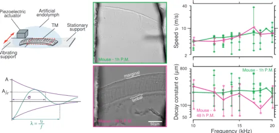
Human TM wave properties could not be measured immediately following death due to the time it takes to obtain TM samples. Therefore, all TM wave measurements across human and mouse preparations were performed roughly 48 hrs post-mortem. To test how mouse TM wave properties change as a function of time, we measured TM wave properties over a 48-hr time period and found that mouse TM wave decay constants were indistinguishable at 1-hr and 48-hr post-mortem (Fig. 2).

50 µm Speed υ (m/s) Decay constant σ ( µ m) 100 Frequency (kHz) 10 20 10 Mouse - 48 h P.M. Mouse - 1h P.M. 50 800 2 40 Mouse - 1h P.M. limbal marginal Mouse - 48 h P.M. Vibrating support Artificial endolymph TM Piezoelectric actuator Stationary support A Ae λ = σ σ υ f / 15

FIGURE 2. Effect of time on mouse TM properties. Left panels: schematic representation of the setup (top) and parameters of an exponentially decaying traveling wave (bottom). Middle panels: Mouse TM images at 1hr and 48hr post-mortem. Right panels: TM wave speed in mouse TMs at 1 hr (n = 10) and 48 hrs (n = 4) post-mortem (top). TM wave decay constant in mouse TMs at 1 hr and 48 hrs post-mortem (bottom).

RESULTS: INTERSPECIES TM MORPHOLOGY

TM samples obtained from humans were expectedly similar in structure and shape to those obtained from rodents. In Fig. 1, we show a representative TM sample from the basal regions of the two species measured. Taking the distance from the marginal band of the TM to the limbal edge, henceforth referred to as WT M, we see roughly a factor of two

difference between WT Mvalues in samples from mice and humans taken from analogous regions of the cochlea (table

1). This distance marks the width of the side of the organ of Corti on top of the hair bundles, suggesting that despite the factor of 100 difference in body size of these mammals, the width of the organ of Corti, and by extension, the diameter of hair cells, do not differ as greatly. We compared our data of TM width to previous measurements of BM width in these two species [15, 16]. We found that in both species, the TM and BM have comparable widths in the base. Although the overall TM length varies from approximately 7 mm in mice to 35 mm in humans, the width and longitudinal spacing of individual collagen fibers in TMs from these animals do not differ significantly (table 1).

The next parameter that we measured in the table below is the distance between TM fibers, ∆f ibers. In order to

measure this parameter, we measured the distance between six fibers near the marginal band of each TM then divided our measurement by 5. We found this parameter to be close to 2 µm in human TMs and half a micron less in mouse TMs. Previously, the spacing of fibers has been associated with shear modulus of the TM [17]. Therefore, from the fiber spacing alone, we would predict some difference in shear moduli for human and mouse basal TM samples.

A systematic difference that we observed in TM samples obtained from humans compared to mice is the orien-tation of collagen fibrils in the TM. In human TM samples, the angle the collagen fibrils make relative to the radial cochlear direction, φf ibers, is larger than in mice. This can be seen in Fig. 1 and is quantified in table 1. This was

observed in all human TM samples and is consistent with previous observations of human TM morphology [18]. The angle of TM fibers could affect TM shear modulus and the direction of the TM wave propagation.

The next parameters in the table relate to Hensen’s stripe including its width, WHS, and the length of a

perpendic-ular line drawn from the marginal band to the closest edge of Hensen’s stripe, DMBtoHS. For each of these, we divide

the parameter by the TM width to determine the approximate fraction that they cover. For the distance between the marginal band and Hensen’s stripe, we found that Hensen’s stripe was generally positioned roughly in the center of the TM.

A consistent difference in TM morphology across the species studied was the structure of Hensen’s stripe. We observed that the width of Hensen’s stripe, WHS, was a significantly larger fraction of the overall TM width, WT M,

in human samples compared to those from mice. When viewing TM samples under high magnification as shown in Fig. 1, we changed the focal plane to determine the minimum width of Hensen’s stripe and found this parameter to be significantly higher in humans than in mice. The percentage of TM width covered by Hensen’s stripe is 10 - 15% in

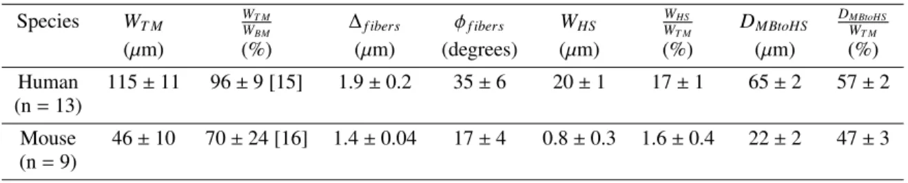
TABLE 1. WT M: width of the TM from the marginal band to the limbal edge,W_WT M_BM: width of TM as a fraction of width of

the basilar membrane, ∆f ibers: spacing of collagen fibers in the TM, φf ibers: angle of collagen fibers relative to the marginal

band in human and mouse samples. All values are represented as median ± half interquartile range.

Species WT M W_WT M_BM ∆f ibers φf ibers WHS _WW_{T M}HS DMBtoHS DMBtoHS_{WT M}

(µm) (%) (µm) (degrees) (µm) (%) (µm) (%)

Human 115 ± 11 96 ± 9 [15] 1.9 ± 0.2 35 ± 6 20 ± 1 17 ± 1 65 ± 2 57 ± 2

(n = 13)

Mouse 46 ± 10 70 ± 24 [16] 1.4 ± 0.04 17 ± 4 0.8 ± 0.3 1.6 ± 0.4 22 ± 2 47 ± 3

(n = 9)

humans; whereas, in mice this parameter is between 1-2%. Despite previous observations of unfixed human cochlear tissue [18] and isolated fixed human TM samples [20], to our knowledge, this is the first comparison of Hensen’s stripe morphology between humans and other mammals in unfixed TM samples. However, this band-like Hensen’s stripe has also been observed in previous studies of TM microstructure in other mammals [21]. In approximately half of the human basal TM samples, Hensen’s stripe was not visible. In a few cases, it was present in half of the TM sample and torn off in the other half. We observed on occasion that Hensen’s stripe visibly came off from the TM sample during extraction from the cochlea.

RESULTS: INTERSPECIES TM PHYSIOLOGY

Of all the TM samples used for the morphological study, only a few yielded wave motions with large enough amplitude and enough contrast to be included in the study of wave motions between humans and mice. The measured wave decay constants (σ) and speeds (ν) for human and mouse TMs show significant overlap of the median and ranges (Fig. 3B). The wave speeds of TM traveling waves in human samples increase by roughly a factor of two from 5 to 20 kHz. Mouse TM speeds also increase with frequency, nearly overlapping human speeds for the physiologically relevant range of frequencies (10-20 kHz). The median decay constants of human TMs range from 150 and 450 µm from 5 to 20 kHz and are relatively constant with frequency. Similarly, the range of median σ-values for mouse TMs is 80-300 µm from 10 to 20 kHz. Overall, our human and mouse speeds and decay constants are quite similar across the overlapping frequency range of hearing.

The wave properties of viscoelastic gels depend on dynamic material properties, including density, ρ, shear storage modulus, G′_{, and shear viscosity, η [9]. We used a lumped parameter model consisting of a distributed series}

of masses coupled by viscous and elastic elements [9] and computed the material properties for each TM wave measurement. We found that across all of the TM samples considered, there was no significant difference between human (G′_{=14.5 ± 8.2 kPa and η = 0.16 ± 0.1 Pa·s) and mouse (G}′_{=16.3 ± 6.6 kPa and η = 0.21 ± 0.1 Pa·s) dynamic}

material properties.

Spatial decay constants, σ, for mice and human TM samples are on the order of 150 µm at 20 kHz (Fig. 3B). Using the cochlear space-frequency map for mice (Fig. 3A), a σ value of 150 µm corresponds to a frequency spread of 1.6 kHz and therefore a quality of tuning Q10dBof approximately 10 at 20 kHz [10]. In TectB knockout mice, the

decay constant of TM waves is roughly halved, leading to a Q10dBvalue that is doubled [10]. In these mutant mice,

sharpened tuning predicted from the mechanical spread of excitation measured in an isolated TM strongly correlates with sharpened neural tuning [13].

Using the cochlear space-frequency map for humans (Fig. 3A), we found that TM waves span significantly different ranges of frequencies (Fig. 3C) in humans. For the mouse, σ = 150 µm corresponds to a frequency range of 1.6 kHz, while the same distance corresponds to <300 Hz in humans. This difference suggests that the spread of excitation via TM traveling waves is broader in mice than in humans. We therefore characterize spread of excitation in terms of the range of frequencies over which the excitation is spread. Because the relation between cochlear location and best frequency is approximately logarithmic [13, 25], constant distances map to logarithmic frequency ranges, such as octaves. We converted TM wave decay constants from distances (in meters) to frequency ranges (in octaves) by dividing σ by the distance D over which frequency changes by one octave. By normalizing decay constants for mice and humans, we found significant differences in frequency spread of excitation between the two species (up to a factor of 4 reduction in human spread of excitation compared to mice) (Fig. 3C). Thus, normalizing the wave decay

Speed υ (m/s) Decay constant σ ( µ m) A 100 Frequency (kHz) 10 5 10 20 Mouse - 48 h P.M. Human - 48 h P.M. Human - 48 h P.M. B 2 mm D = 5 mm D=1.25 mm octave base apex C Normalized decay constant σ/ D (octaves) 0.1 0.01 10 1 Normalized speed ν/ D (k-octaves/s) Frequency (kHz) 5 10 20 2 600 50 0.4

FIGURE 3. Human and mouse TM wave properties. (A) Schematic drawings of human and mouse cochlear spirals highlighting the distance over which frequency changes by a factor of two. (B) Speeds and decay constants for humans and mice in m/s and m, respectively. (C) TM speeds and decay constants normalized by distance D to include the effect of the cochlear map. Adapted from [19]

constant to reflect the physiologically important range of frequencies reveals striking differences between humans and mice.

DISCUSSION

The goal of this study was to compare the morphologies and physiological properties of the tectorial membranes of mice and humans. Several morphological properties were found to differ in these species, and two seem most likely to affect material properties. First, the distance between radial fibers in humans is about 35% greater than it is in mice. If all other factors were similar, reducing the radial fiber density would tend to decrease the elastic modulus. However, the angle between the fibers and the marginal edge in the human TM is significantly greater than that in the mouse. The greater angle could tend to increase radial stiffness, as more fibers could contribute to radial shear. Given these opposing trends, it is perhaps not surprising that we measured little difference in material properties.

Traveling wave properties of the human and mouse TMs were also found to be similar. For frequencies between 10 and 20 kHz, the median wave propagation velocities ranged from 4-10 m/s, and the median wave decay constants ranged from 100-300 µm. However, these wave decay constants correspond to significantly different ranges of best frequencies, as defined by the cochlear maps for humans and mice.

Q 10 1 Human Human Frequency (kHz) 5 10 20 10dB SFOAE_(Dreisbach et al, 1998) 100 Mouse Frequency (kHz) 5 10 20 SFOAE (Cheatham et al, 2015) TM waves TM waves TM waves SFOAE (Banakis and Siegel , 2008) SFOAE (Shera et al, 2002)

FIGURE 4. Relating TM wave decay to sharpness of tuning in mice and humans. Q10dB predictions for humans (left panel)

and mice (right panel) based on TM wave decay constants compared to Q10dB predictions from stimulus frequency otoacoustic

emissions (SFOAEs) for humans [22, 6] and mice [23, 24]. The SFOAE estimates are calculated from the phase delay of SFOAE measurements as described in [6]

a quality of tuning (Q10dB). Figure 4 shows significantly larger Q10dBpredicted from TM spatial decay constants in

humans compared to mice (larger by a factor of four), consistent with a smaller spatial extent of TM waves relative to the cochlear map. These Q10dBpredictions based on TM wave decay constants are comparable to cochlear tuning

predictions based on otoacoustic emissions [6]. Previous studies have shown these emission-based estimates of tuning to be comparable to neural estimates for a range of mammalian species [6, 7, 8]. For mice, the quality of tuning estimated from TM wave decay constants closely matches predictions of Q10dBfrom otoacoustic emissions [23]. For

humans, the Q10dBestimates are comparable to emissions-based estimates [22] from 5 to 10 kHz. These findings

suggest that the spatial extent of TM traveling waves contributes to differences in cochlear tuning in humans and other mammals.

ACKNOWLEDGMENTS

This work was supported by NIH grant R01-DC00238. SF and JBS were supported in part by a training grant from the National Institutes of Health to the Speech and Hearing Biosciences and Technology Program in the Harvard-MIT Program in Health, Sciences, and Technology. The authors would like to thank Diane Jones for dissecting the human temporal bones from donors. We also thank Christopher A. Shera, John J. Guinan Jr, and Scott L. Page for their helpful comments and suggestions on this work.

REFERENCES

[1] M. A. Ruggero and A. N. Temchin, Proc Nat Acad Sci 102, p. 1861418619 (2005).

[2] A. Eustaquio-Martn and E. A. Lopez-Poveda, J Assoc Res Otolaryngol 12, 281–299 (2010). [3] Y. Bitterman, R. Mukamel, R. Malach, I. Fried, and I. Nelken, Nature 451, 197–201 (2008). [4] R. V. Harrison, J.-M. Aran, and J.-P. Erre, Jour. Acoust. Soc. Am. 69, 1374–1385 (1981).

[5] J. M. Sinnott, M. D. Beecher, D. B. Moody, and W. C. Stebbins, Journ. Acoust. Soc. Am. 60, p. 687 (1976). [6] C. Shera, J. Guinan, and A. Oxenham, Proc. Nat. Acad. Sci. 99, 3318–3323 (2002).

[7] C. Shera, J. Guinan Jr, and A. Oxenham, Journ. Assoc. Res. Otol. 11, 343–365 (2010).

[8] P. Joris, C. Bergevin, R. Kalluri, M. McLaughlin, P. Michelet, M. van der Heijden, and C. Shera, Proc. Nat. Acad. Sci. 108, 17516–20 (2011).

[9] R. Ghaffari, A. J. Aranyosi, and D. M. Freeman, Proc. Nat. Acad. Sci. 104, 16510–16515 (2007). [10] R. Ghaffari, A. J. Aranyosi, G. P. Richardson, and D. M. Freeman, Nat. Comm. 1 (2010).

[11] J. B. Sellon, S. Farrahi, R. Ghaffari, and D. M. Freeman, Proc. Nat. Acad. Sci. 112, 12968–12973 (2015). [12] H. Y. Lee, P. D. Raphael, J. Park, A. K. Ellerbee, B. E. Applegate, and J. S. Oghalai, Proc. Nat. Acad. Sci.

[13] I. J. Russell, P. K. Legan, V. A. Lukashkina, A. N. Lukashkin, R. J. Goodyear, and G. P. Richardson, Nat. Neuro. 10, 215–223 (2007).

[14] N. Wadhwa, M. Rubinstein, F. Durand, and W. Freeman, ACM Transactions on Graphics (TOG) 32, p. 80 (2013).

[15] C. Fern´andez, The Journal of the Acoustical Society of America 24, p. 519 (1952). [16] H. Burda, L. Ballast, and V. Bruns, Journal of morphology 198, 269–285 (1988).

[17] B. Shoelson, E. K. Dimitriadis, H. Cai, B. Kachar, and R. S. Chadwick, Biophys J 87, 2768–2777 (2004). [18] G. von B´ek´esy, Experiments in Hearing (McGraw-Hill, New York, 1960).

[19] S. Farrahi, R. Ghaffari, J. B. Sellon, H. H. Nakajima, and D. M. Freeman, Biophys J Letters 111, 921–924 (2016).

[20] T. Hoshino, Archives of oto-rhino-laryngology 217, 53–60 (1977). [21] D. J. Lim, Hear Res 22, 117–146 (1986).

[22] L. E. Dreisbach, J. H. Siegel, and W. Chen, Ass. Res. Otol. Abstr. 21 (1998).

[23] M. A. Cheatham, R. J. Goodyear, K. K. Charaziak, T. Conklin, J. Zheng, P. Dallos, G. P. Richardson, and J. H. Siegel, in Mech. Hear., edited by K. D. Karavitaki and D. P. Corey (American Institute of Physics, 2015).

[24] R. Banakis and J. Siegel, “Spontaneous and tone-evoked otoacoustic emissions in mice,” in Abstracts of the Thirty-first Midwinter Research Meeting(Association for Research in Otolaryngology, Phoenix, Arizona, 2008).

[25] D. D. Greenwood, Journ. Acoust. Soc. Am. 87, 2592–2605 (1990).

COMMENTS AND DISCUSSION

1. Stefan Raufer:

Comment: Fig. 4: The results from Dreisbach et al. (1998) shown in Fig. 4 match your data well, but do only reflect one out of many approaches to measure cochlear tuning in humans. They seem extraordinary high compared to other SFOAE tuning estimates (Shera et al, 2002 PNAS)?

Response: We have added data from other SFOAE tuning estimates to each panel of Figure 4. While the tuning estimated from the Dreisbach, et. al., 1998 and Shera, et. al., 2002 papers differ, the raw SFOAE delays are overlapping (see comparison in Figure 1 of Shera and Guinan, JASA 113(5) 2762-2772). Furthermore, data are sparse above 5 kHz, which is where our TM estimates begin.

Comment: Fig 4: SFOAEs are measured near threshold, where active processes immensely sharpen the cochlear filter. How do you explain that your ex-vivo passive TM measurements reflect the sharp active tuning instead of the less sharp passive tuning?

Response: Previous studies (Ghaffari, et. al., 2010) have shown a correlation between passive TM mechanics and in vivo measurements of cochlear tuning. Although the mechanism behind this correlation is not clear, it is possible that sharp tuning depends not only on active mechanisms (such as outer hair cell motility) but also on passive coupling through the TM (as has previously been suggested for passive coupling through cochlear fluids).

2. MaryAnn Cheatham:

Comment: Having the human TM results is a welcome addition to your work and the species comparisons are important. From the Methods, it appears that the segments were taken from the base of the cochlea in both species, yet the stimuli were 5-20 kHz. In humans, this range corresponds to basal CFs but in mouse to apical CFs. The latter is based on the mouse frequency place map (Mller et al., 2005) where the middle of the cochlea is the 20k place.

Response: We extracted portions of the mouse TM from the entire basal turn, so the center frequencies range from roughly 10-60 kHz. We only reported frequencies up to 20 kHz, because that is the maximum frequency that is possible with our current wave chamber.

Question: I am also confused by the measurements of TM width in the mouse. Your width measurements (46 µ) do not compare with those of Keiler and Richter (2001) where the TM width increased from 120 µ in the apex to 200 µin the base. They measured from the MB to the limbal attachment. How does this compare to your measurements from the MB to the limbal edge? I am also confused by the median of 46 µ in Table 1 as this is much narrower that the distance between BM and limbus in Fig. 2 where the width of the TM is slightly greater than 100 µ based on the calibration bar. In fact, the TM widths are different in Fig. 1 and Fig. 2 (48 hr) for the mouse. In Fig. 1, I as-sumed that the human and the mouse TM images were both obtained at 48 hr to foster the comparisons. Please clarify. Response: Thank you for pointing out the difference between our measurements and images. The images included in the initial draft were in fact not representative of the majority of images from this study. While all of the mouse specimens came from the basal turn, some (such as the one in the initial draft) were more apical than others. We have updated the images to be more representative of those included in the associated data plots. You are correct that the mouse and human TM images in this paper were both obtained 48 hours post-mortem.

Comment: Although the SFOAE/TM tuning estimates are comparable for 5-20 kHz, Manley and van Dijk (2016) indicate that below 5 kHz SOAE suppression tuning curves in humans match psychophysical estimates and both at broader than the SFOAE estimates. To be conservative, perhaps one should acknowledge that SFOAE estimates of tuning may not be as accurate at low frequencies in some species.

Response: This is a good point. We agree that we cannot draw any conclusions about frequencies below 5 kHz in this study.

3. Julien Meaud:

Comment: I enjoyed reading your manuscript. I found it very interesting that you are charcterizing wave propagation on isolated human tectorial membranes. The fact that you are observing similar wave parameters despite significant morphological differences, including fiber direction, is unexpected.

Response: We also expected to see a difference in TM wave properties due to differences in human TM morphology, but differences were small.

Question: Fig 1 shows that the human TM is less curved than the mouse TM. Do you think it is true in vivo, or is it and artifact of your in vitro experimental procedure? This could affect wave propagation on the TM.

Response: The smaller curvature of the human TM in Figure 1 is representative of other human TMs in this study. In all cases, we tried to mount the isolated TM segments without changing their natural curvature. The smaller curvature is consistent with the larger size of the human cochlear spiral.

Question: Where exactly is the radial displacement measured? At the Hensens stripe?

Response: The radial displacement is measured at Hensens stripe. This position is near that of the hair cells, and also provides greater contrast than other regions (which is important for our motion analysis). We have added a note to this effect to the Methods section of the text.

Question: Some of your postportem individual measurements for the decay constant are very large ( 800 microns). Given that the length of TM is likely shorter than this, how confident are you about this value?

Response: These large decay constant measurements are only seen at a few low frequency points in the human samples. As you point out, our measurements are most accurate when the distance between the two points of TM attachment is large compared to the wave decay constant. For that reason, we routinely adjusted the supports to maximize the distance for TM segments with different lengths. This wider gap is the reason that the stationary support is often not visible in the human TM images.

4. Jont Allen

created the field, and the frequency just noticeable difference (JND) for pure tones is about 20x higher resolution than the critical band. The JND being 20x smaller than the critical band means that bandwidth is not the determinant of frequency selectivity which you started your talk with. Fletcher believed that the way you discriminate a JND for pure tones is off the high f edge of the cochlear slope, so it’s basically like an FM discriminator which converts the frequency change to a amplitude change, so I’m suggesting you rethink the initial argument.

Response: We regret any confusion caused by our introducing the talk with reference to the extraordinary frequency selectivity that we as humans possess. We agree completely that frequency discrimination is far too sharp to be based solely on the bandwidth of cochlear filters.

5. Robert Harrison

Comment: Along the same line of thought. Frequency selectivity and JND are two different things. Psychophysicists have measured critical bands and psychophysical tuning curves in animals and humans. They’re not all that different. I myself have derived the frequency tuning of neurons in the human cochlear nerve as has Jos Egermont using tone on tone forward masking paradigms. They’re not much different from guinea pigs, gerbils, cats, so your initial premise about the frequency selectivity of the human being better than other mammalian species is just incorrect.

Response: We regret any confusion caused by our introducing the talk with reference to the extraordinary frequency selectivity that we as humans possess. Our study was intended to compare cochlear mechanisms in humans and mice and to look for similarities and differences. We have added several references to better reflect the lack of consensus on the relative sharpness of human frequency tuning.

6. Andrew Oxenham

Comment: I disagree with Robert Harrison’s statement. There’s a lot of disagreement on this topic. It’s not a closed case and I think there’s actually strong evidence that human tuning is sharper than animal tuning measured in several different ways by a factor of two or three.

7. Chris Bergevin

Question: Out of curiosity in the human temporal bones, what was the state of the hair cells?

Response: In the TM extraction process, we destroyed the entire organ of Corti aside from the TM, so we were not able to visualize the hair cells.