HAL Id: hal-01802488
https://hal.inria.fr/hal-01802488
Submitted on 29 May 2018
HAL is a multi-disciplinary open access
archive for the deposit and dissemination of
sci-entific research documents, whether they are
pub-lished or not. The documents may come from
teaching and research institutions in France or
L’archive ouverte pluridisciplinaire HAL, est
destinée au dépôt et à la diffusion de documents
scientifiques de niveau recherche, publiés ou non,
émanant des établissements d’enseignement et de
recherche français ou étrangers, des laboratoires
Instrumenting a Weakest Precondition Calculus for
Counterexample Generation
Sylvain Dailler, David Hauzar, Claude Marché, Yannick Moy
To cite this version:
Sylvain Dailler, David Hauzar, Claude Marché, Yannick Moy. Instrumenting a Weakest Precondition
Calculus for Counterexample Generation. Journal of Logical and Algebraic Methods in Programming,
Elsevier, 2018, 99, pp.97-113. �hal-01802488�
Instrumenting a Weakest Precondition Calculus for
Counterexample Generation
ISylvain Daillera,b, David Hauzara,b,c, Claude March´ea,b,∗, Yannick Moyc
aInria, Universit´e Paris-Saclay, F-91120 Palaiseau bLRI, CNRS & Univ. Paris-Sud, F-91405 Orsay
cAdaCore, F-75009 Paris
Abstract
A major issue in the activity of deductive program verification is to understand why automated provers fail to discharge a proof obligation. To help the user understand the problem and decide what needs to be fixed in the code or the specification, it is essential to provide means to investigate such a failure. We present our approach for the design and the implementation of counterexample generation, exhibiting values for the variables of the program where a given part of the specification fails to be validated. To produce a counterexample, we exploit the ability of SMT solvers to propose, when a proof of a formula is not found, a counter-model. Turning such a counter-model into a counterexample for the initial program is not trivial because of the many transformations leading from a particular piece of code and its specification to a set of proof goals given to external provers.
Keywords: Deductive Program Verification, Weakest Precondition Calculus,
Satisfiability Modulo Theories, Counterexamples
1. Introduction
Deductive program verification is an activity that aims at checking that a given program respects a given functional behavior. In this context, the ex-pected behavior must be expressed formally by logical assertions, i.e. precon-ditions and postconprecon-ditions, forming a contract. Deductive program verification proceeds by generating, from both the code and the formal specification, a set of logic formulas called verification conditions (VCs), typically via a Weakest Precondition Calculus [1] (WP for short). If one proves all generated VCs, then the program is guaranteed to satisfy its specification. In recent program verifi-cation environments like Dafny [2], OpenJML [3] and Why3 [4], VCs are proved
IWork partly supported by the Joint Laboratory ProofInUse (ANR-13-LAB3-0007, http:
//www.spark-2014.org/proofinuse) of the French national research organization
using automated theorem provers, in particular those of the Satisfiability Mod-ulo Theories (SMT) family such as Alt-Ergo [5], CVC4 [6] and Z3 [7]. These theorem provers are used as black-boxes that, given a VC, may produce three kinds of results:
1. The prover answers something meaning “yes, the VC is valid”.
2. The prover answers anything else, meaning “I don’t know”, in other words the prover is not able to prove the VC for some reason.
3. The prover runs for too long a time (seemingly infinitely) or runs out of memory.
The case where the prover runs for too long a time is handled in practice by setting a given time limit, so that the prover process is killed when exceeding this limit. The cases 2 and 3 are the same from the user’s perspective: the VC is not proved. Note that we do not distinguish a case where the prover would answer “no it is not valid”, because the VCs typically involve undecidable logic features (e.g. non-linear integer arithmetic, first-order quantification) so provers are in practice incomplete: there is no way for them to be sure that a given VC is not provable.
A major issue in the activity of deductive verification is thus understanding the reasons for a proof failure. There are various reasons why it may fail:
1. The property to prove is indeed invalid: the code is not correct with respect to the given specification.
2. The property is in fact valid, but is not proved, again for two possible reasons:
• The prover is not able to obtain a proof (in the given time and mem-ory limits): this is the incompleteness of the proof search.
• The proof might need extra intermediate annotations, such as loop invariants, or more complete contracts of the subprograms.
For the user to be able to fix the code or the specification of their program, it is essential to understand into which of these two cases any undischarged VC falls. The solution we propose in this paper is to generate counterexamples, giving values for the variables of the program, demonstrating a particular case where a given annotation may not hold. To produce a counterexample, we exploit an additional feature of SMT solvers: the ability to propose, when a proof of a formula is not found, a counter-model, exhibiting an interpretation of the free variables where the formula cannot be proved true. Turning such a counter-model into a counterexample for the initial program is not a trivial task because of the many transformations that lead to a VC from a given piece of code and its specification. It is important to notice here that because of the sources of incompleteness mentioned above, this process can only produce candidate counterexamples, in the sense that they do not necessarily exhibit an error in the code or in the specification. Given a counterexample, the user must analyze it to decide if it corresponds to a true bug or to an incompleteness (such as an extra loop invariant required).
Java programs C programs Ada programs
Krakatoa Frama-C/Jessie SPARK 2014
WhyML programs VC generator
Proof tasks in Why3 logical framework Encoders/Printers
SMT solvers
TPTP provers Interactive provers
Figure 1: Why3 ecosystem
The work presented here was conducted in the context of the Why3 envi-ronment for deductive program verification (http://why3.lri.fr), providing the language WhyML for specification and programming [8]. WhyML is used as an intermediate language for verification of programs written in C, Java or Ada [9, 10]. A schematic view of the Why3 ecosystem is shown in Figure 1. The specification component of WhyML [11], used to write program annotations and background theories, is an extension of first-order logic. The specification part of the language serves as a common format for theorem proving problems, proof tasks in Why3’s jargon. Why3 generates proof tasks from user lemmas and an-notated programs, using a weakest-precondition calculus, then dispatches them to multiple provers. Other deductive verification environments are structured in a similar way, for example the Boogie intermediate language [12] serves as an intermediate language for Spec#, VCC or Dafny, implements its own variant of a WP calculus, and dispatches the VCs to the SMT solver Z3. The approach we present here for counterexample generation thus applies to other environ-ments as well, the main issue being how to trace the counter-model proposed by SMT solvers back through the WP calculus and furthermore back through the encoding of front-end languages to the intermediate language.
Our approach for generating counterexamples for the SPARK 2014 front-end was originally presented at the SEFM conference in 2016 [13]. The current article investigates in a more generic manner the issues we had to solve, and details the technical solutions we designed. We also present a technique for handling arrays that is different from the previous version. The experimental evaluation is updated with results of the newer implementation, with the new handling of arrays but also a few implementation bugs fixed. Also, it does not only make use of the CVC4 solver but also Z3. In Section 2, we present the design of an instrumentation of the WP calculus, aiming at keeping track
of source code data inside the generated formulas. The transformations of proof goals, which need to be performed before sending the VCs to external provers, are instrumented as well. In Section 3, we focus on the additional instrumentation work that was needed to handle compound data types such as records and arrays. In Section 4 we then present the extra instrumentation needed to bring the counterexamples back to front-end languages. We present an experimental evaluation of the implementation of our approach in Section 5. We discuss related work and future work in Section 6.
2. Instrumenting a Weakest-Precondition Calculus
The VC generators found in deductive verification environments typically implement some variant of Dijkstra’s Weakest-Precondition Calculus. To illus-trate how a WP calculus should be instrumented for counterexample genera-tion, we consider a simple “while” language with assignment, conditionals, while loops and subprogram calls. The issues to solve show up mainly in the handling of assignment, loops and calls, and they are the same independent of the WP calculus variant.
2.1. A Basic VC Generator for a Simple While Language
The statements of the simple programming language we consider are defined by the grammar
s ::= skip (no operation)
| x := e (assignment)
| assert P (assertion)
| s1; s2 (sequence)
| if e then s1 else s2 (conditional)
| while e invariant I do s (loop)
| p(e1, . . . , en) (subprogram call)
For simplicity of the presentation, let us assume that procedures only oper-ate on variables that are defined globally, and that procedure parameters are immutable.
The computation of the weakest-precondition WP(s, Q) for a given state-ment s and postcondition Q is done recursively on the structure of s, using the rules of Figure 2. These are very standard rules, not trying to optimize the size of generated formulas (See [14, 15, 16] for more elaborate WP calculi). It is enough to consider such a basic WP calculus for our purpose, since it is the introduction of fresh variables that raises the main issue for counterexample generation: the relation between each fresh variable and a variable in the orig-inal program must be traced. Indeed, the variables ~v universally quantified in the rules for assignment, loops and procedure calls must be assumed to be fresh ones. The notation Q[x ← v] denotes the substitution of v for x in formula Q. The connective && is asymmetric conjunction discussed later in Section 2.2. Note the formulation of the rule for assignment, which differs from the standard
WP(skip, Q) = Q
WP(x := e, Q) = ∀v. v = e → Q[x ← v]
WP(assert P, Q) = P && Q
WP(s1; s2, Q) = WP(s1, WP(s2, Q))
WP(if e then s1 else s2, Q) = if e then WP(s1, Q) else WP(s2, Q)
WP(while e invariant I
do s, Q) = I ∧
∀~v. (I →
if e then WP(s, I) else Q)[ ~w ← ~v] where ~w are the variables modified in the loop body
WP(p(e1, . . . , en), Q) = P rep[xi← ei] ∧
∀~v. (P ostp[xi← ei] → Q)[ ~w ← ~v]
where ~w are the variables modified by subprogram p(x1, . . . , xn)
Figure 2: Rules for WP computation
formulation Q[x ← e]. Our formulation has two advantages: first, it avoids the potential duplication of expression e (that is for each occurrence of x in Q), and second, the fresh variable v introduced will be labelled so as to track information from the source code.
Generally speaking, when a given subprogram procedure p(x1, . . . , xn) = s
is formally specified with some precondition P repand postcondition P ostp, its
verification condition is the logic formula
∀~x, ~v.(P rep→ WP(s, P ostp))[~r ← ~v]
where ~r are the global variables read by p.
We now introduce two toy procedures that will serve as running examples for illustrating the process of counterexample generation through the rest of this section. Note that these examples are intentionally chosen to be incorrect, so that the generation of counterexamples is expected.
Example 1. The procedure p1is defined as follows, operating on a global
vari-able a. procedure p1 (b:int) requires { 0 ≤ a ≤ 10 ∧ 3 ≤ b ≤ 17 } ensures { 17 ≤ a ≤ 42 } = a := a + b; assert { 5 ≤ a ≤ 15 }; if a ≥ 10 then a := a - 1
It is intentionally crafted so that both the assertion and the postcondition are not valid. Its VC as computed by our WP calculus is the following formula
∀a b. (0 ≤ a ≤ 10 ∧ 3 ≤ b ≤ 17) → ∀a1. a1= a + b →
(5 ≤ a1≤ 15) &&
Example 2. The procedure p2 is defined as follows, using two global variables a and c. procedure p2 () requires { 0 ≤ a ≤ 10 } ensures { 7 ≤ a ≤ 42 } = c := 1; while c ≤ 10 do invariant { 2 ≤ c ≤ 11 } invariant { 3 ≤ a ≤ 10 } a := a + c; c := c + 2 done
This toy example is crafted so that all verification conditions are unprovable. First the loop invariants are not initially true, and they are not preserved by loop iterations. Second the postcondition is also unprovable, but there is a subtlety here: the postcondition is indeed valid for each execution of that procedure (the final value of a is indeed between 25 and 35), but it cannot be proved with only the knowledge of the loop invariant. The VC for p2 is
∀a. (0 ≤ a ≤ 10) → ∀c. c = 1 → (2 ≤ c ≤ 11 ∧ 3 ≤ a ≤ 10)∧ (∀a1 c1. 2 ≤ c1≤ 11 ∧ 3 ≤ a1≤ 10 → if c1≤ 10 then (∀a2. a2= a1+ c1→ ∀c2. c2= c1+ 2 → 2 ≤ c2≤ 11 ∧ 3 ≤ a2≤ 10) else 7 ≤ a1≤ 42)
Note the structure of the generated formulas: only universal quantification is introduced, and always in positive positions of the formula (i.e. in the right side of implications and never under negation).
2.2. Proof Tasks and Transformations
The VC formula generated for a given procedure is typically quite large, as it collects all the necessary checks that need to hold for the function to be correct: postcondition, initialization and preservation of loop invariants, all run-time checks, etc. Such a big formula could be given as is to a theorem prover, but then one would get just a yes/no answer for the correctness of the whole procedure, or no answer at all. It is thus better to first transform the VC, splitting it into smaller parts called proof tasks, before calling a back-end solver. Indeed, to successfully obtain a counterexample from a call to an SMT solver, the universally quantified variables must be defined at the top-level, it is thus mandatory to transform the VC into a set of clauses.
Definition 3. A proof task is a combination of a set of hypotheses H1, . . . , Hn
and a goal G, written as H1, . . . , Hn ` G. It is said to be valid when G is a
logical consequence of the hypotheses, for all values of the free variables. A trans-formation is any procedure taking a proof task as an argument and producing a set of proof tasks.
Transformations are expected to be sound in the sense that validity of the resulting tasks must imply the validity of the input task. The converse does not need to hold.
The two following sound transformations are of utmost importance for han-dling formulas generated by WP.
• Introduction of premises is the transformation that moves prenex uni-versally quantified variables and left parts of implications into the set of hypotheses, that is a task H ` ∀x. H1→ G is transformed into H, H1` G.
Note that the bound variable x becomes a free variable in the resulting proof task.
• Splitting is the transformation that, given a proof task of the form H1, . . . , Hk ` G1∧ · · · ∧ Gn, produces the set of n tasks H1, . . . , Hk ` Gi
for 1 ≤ i ≤ n.
Indeed, these transformations are typically applied eagerly on formulas gener-ated by WP, in order to obtain a set of tasks that are easily associgener-ated with expected properties like “overflow check”, “preservation of a loop invariant”, etc.
Example 4. The VC for our running example p2can be split into 5 proof tasks.
The first task is
H1 : 0 ≤ a ≤ 10
H2 : c = 1
G : 2 ≤ c ≤ 11
It corresponds to proving that the first loop invariant is initially true.
Note that in practice, Why3 implements a general infrastructure for task transformations, allowing the user to easily implement new transformations us-ing combinators. As most of the provers do not support some of the logic lan-guage features (e.g. in Why3: pattern matching, polymorphic types, recursion), Why3 applies a series of encoding transformations to eliminate unsupported con-structions before dispatching a proof task to provers. Other transformations can also be imposed by the user in order to simplify the proof search: in-lining of def-initions, simplification by computation, case analysis, application of inductive schemes, etc.
2.3. Tracing Information Using Labels
We are now ready to introduce our first technical mean for tracing informa-tion: labels attached to formulas.
Definition 5. A label is an arbitrary character string, written between double quotes. It can be attached to any logic formula or term, and also to any identifier declaration.
The purpose of labels is to keep track of information during the process of transforming proof tasks. The labels have no interpretation fixed a priori. They have meaning in the context of particular task transformations.
Example 6. The asymmetric conjunction operator written as &&, does not need to be a new specific connective in the logic language. It can be seen as the usual conjunction ∧ with a specific label "asym_split". The splitting transformation can interpret this label so that a goal of the form f1 && f2 is split into the
sub-goals f1 and f1→ f2, producing the expected behavior that f1 is assumed true
in the right part of the conjunction.
Transformations that do not interpret labels should keep them attached to formulas and terms, if possible. For example, a transformation may rename a variable, in that case it should propagate labels from the original variable to the new one. Analogously, if a transformation rewrites a given sub-term into another, it should also propagate labels of the old term to the new one. Example 7. Labels can be used for the sub-tasks explanations: to make the proof tasks presentation more user-friendly, WP calculus can be instrumented so that each of the sub-formulas that corresponds to a program check is anno-tated with a label meaningful for humans. In Why3, those labels have the form "expl:text" where text is a human-readable explanation of the VC, which is displayed by the graphical interface.
2.4. Calling an SMT Solver on Proof Tasks
An SMT solver takes as input a set of formulas, and checks whether this set is satisfiable or not. To prove that a given proof task H ` G is valid, we query the solver for the satisfiability of the conjunction H ∧ ¬G. If the solver answers that this set is unsatisfiable, it means that proof task is valid. If the solver terminates with any other answer, the SMT solver may propose a potential model of H ∧ ¬G describing why H ` G cannot be proved. To get such a model, we use features of SMT-LIB [17]: SMT-LIB defines commands get-model and get-value for getting models. The command (get-model), without argument, returns a set of interpretations for all user-declared function symbols in the input task. The command (get-value t1 · · · tn) returns for each term ti a
value term that is equivalent to ti in the potential model.
Example 8. From the proof task of Example 4, an SMT solver will provide a model where c = 1 and a is given any value between 1 and 10. This model validates the hypotheses but not the conclusion, and is a direct counterexample for the initialization of the first loop invariant.
2.5. Interpreting Solver’s Model at the Code Level
Interpreting the model returned by the solver at the level of the initial pro-gram is not always as easy as shown in Example 8. The first step is to trace the fresh variables introduced by the WP calculus back to variables of the original code, at the proper source location. The architecture for this feedback process is shown in Figure 3. First, the initial source code is expected to be annotated by labels that indicate which parts (variables or formulas) are relevant for a
Program code + CE annotations
VC generator Proof tasks +
CE annotations
SMT-LIB printer
SMT queries
mapping of SMT terms
to program variables SMT solver
Model CE at Program level
Transformations
Figure 3: Data-flow for counterexample generation
possible counterexample. The VC generator and then the proof transforma-tions then propagate these labels appropriately. When a given proof task is finally transformed into a corresponding set of SMT-LIB queries, a mapping for SMT-LIB terms to original program variables is also generated. This mapping is used to reinterpret the model returned by the solver into a counterexample at the source level.
We now describe this technical process in detail. 2.5.1. Marking Variables to Show in a Counterexample.
In the design of our approach, we decided that program variables that should appear in a counterexample should be explicitly marked with the label"model". This is needed in particular when the programming language WhyML is used as an intermediate language e.g. for SPARK, as we will see in Section 4.
Example 9. To prepare counterexample generation, the program p1 should be
annotated as follows.
var a "model" : int
procedure p1 (b "model" :int)
requires { 0 ≤ a ≤ 10 ∧ 3 ≤ b ≤ 17 }
ensures { 17 ≤ a ≤ 42 } = a := a + b;
assert { 5 ≤ a ≤ 15 };
The "model" labels are propagated along the VC generation process, in particular each fresh variable introduced by WP inherits the labels of the asso-ciated program variable. In the phase of printing the proof task in the form of a sequence of SMT-LIB queries, we are producing trace data in the form of a mapping M . M associates some terms of the generated SMT problem to some program variable (marked with"model"): if M maps some term t to a variable x, then t represents x.
When the back-end SMT solver is not able to validate a VC, we query it for a counter-model. In the first version of our approach [13], we were using our generated set of terms as the parameters of the get-value command of SMT-LIB. Thus, for each term t queried for a value v in the generated model, we considered v as a value for the program variable associated with t in mapping M . However, this method appeared to be insufficient to handle compound data types like arrays, because the model generated by get-value might not contain all the relevant data. Thus, in the current version, we now use the get-model command to get the whole counter-model and then extract the values of the terms we are interested in. The technical details of this extraction will be given when we handle compound data types in Section 3 .
Example 10. From the running example p1, the proof task for the assertion is
H1 : 0 ≤ a ≤ 10 ∧ 3 ≤ b ≤ 17
H2 : a1= a + b
G : 5 ≤ a1≤ 15
and trace data records that a1 denotes the program variable a after the
assign-ment. For this task, CVC4 returns a model with a = 0, b = 3, a1= 3.
As this example shows, there is still a practical need: how to present to a user the values for variable a both before and after the assignment. To solve this issue, we decided to display the counterexample values at the appropriate source locations, for example the value 3 for a should be attached to the location after the assignment, or at the assertion itself, to distinguish from the value 0 for a that should be attached to the beginning of the procedure body, or at the location of the precondition (see Example 11 below).
2.5.2. Getting Values of Variables at Appropriate Source Locations
To achieve our goal of displaying counterexample values at the appropriate source locations, we assume we can attach to logic variables specific labels that identify source location data: file name and line number. When a fresh variable is introduced by the WP calculus, it is easy to attach to it the source location of the corresponding statement. This technique allows us to attach to the logic variable a1of Example 10 the location of the assignment a := a+b.
We can do even better, in order to achieve what we said above for our running example: we would like to display counterexample values at the source line of the annotations (assertion, postcondition, etc.) involved in the VC. For that purpose we introduce another specific label "model_vc" that we can put
invalidated initial initial a after first a at
condition a b assignment end
assertion 0 3 3
-postcondition (then branch) 0 10 10 9
postcondition (else branch) 0 5 5 5
Figure 4: Counterexamples for each VC of Example 1.
on any logical formula. We implemented a dedicated proof transformation that uses this label: it scans each variable that occurs in the labeled formula, and introduces a fresh copy of it, labeled with the location of the formula itself. This approach allows us to display a counterexample in a user-friendly manner, where the values of the program variables can be displayed interleaved with the source code, at all the locations of interest.
Example 11. Considering again the VC for the assertion in procedure p1, by
annotating the precondition and the assertion with the label "model_vc", our technique allows us to report a failure of the proof of the assertion, and display a counterexample at the location of the assertion and at other locations interleaved with the code (shown in comments), as follows.
procedure p1 (b "model":int)
requires { "model_vc" 0 ≤ a ≤ 10 ∧ 3 ≤ b ≤ 17 } (* a=0, b=3 *)
ensures { 17 ≤ a ≤ 42 }
= a := a + b; (* a=3 *)
assert { "model_vc" 5 ≤ a ≤ 15 }; (* a=3 *)
if a ≥ 10 then a := a - 1
To conclude this section, here is a summary of the counterexamples generated for all the proof sub-tasks of our running examples, using SMT solver CVC4. The counterexamples for procedure p1of Example 1 are shown in Figure 4. The
generated counterexamples are perfectly satisfactory. Note in particular that the counterexamples for the two cases of postcondition failure indeed validate the assertion, which is what we want: a counterexample that would invalidate both the postcondition and the assertion is a good counterexample for the as-sertion but not satisfactory for the postcondition. The reason why this works is because in the VC corresponding to the postcondition, the assertion is part of the premises, so is true in the counter-model proposed by the SMT solver.
The counterexamples for procedure p2of Example 2 are shown in Figure 5.
All generated counterexamples are satisfactory. Counterexamples for loop in-variant preservation validate the loop inin-variant before the considered iteration, counterexamples for postcondition validate the assumed loop invariant at loop exit. We emphasize the subtlety about the postcondition already mentioned in Example 2: indeed the given values that invalidate the postcondition are not reachable by any concrete execution. It is important to remember here that a counterexample produced by our method is only a candidate counterexample,
invalidated condition initial a initial c
initialization first loop invariant 0 1
initialization second loop invariant 0 1
invalidated a before c before a after c after
condition loop loop loop loop
body body body body
preservation first loop inv. 3 10 13 12
preservation second loop inv. 9 2 11 4
invalidated a at c at
condition loop exit loop exit
postcondition 3 11
Figure 5: Counterexamples for each VC of Example 2.
which invalidates the associated proof task but not necessarily the program it-self. As discussed in the introduction, it is left to the user to decide if the given counterexample exhibits a real bug in the code, or if the proof does not proceed because extra annotations should be added (like an appropriate loop invariant in this example), to rule out the candidate counterexample.
3. Support for User-Defined Data Types
So far, we only have programs operating on mathematical integers. We have to cope with a VC generation that also takes care of other data types, such as machine integers, arrays, records, etc. The way such extra data types are handled by various VC generation approaches varies a lot, depending in partic-ular on the support the back-end solvers can provide. For example, supporting machine integers can be done in a straightforward way if the solver natively supports fixed-size bit-vectors, and arrays can be quite efficiently handled if the back-end solver supports the theory of functional arrays.
To handle data types in a general way, we propose a concept of coercion detailed in Section 3.1 below. Additionally, supporting arrays requires a special treatment that we present in Section 3.2. Note that the approach presented here for arrays is completely different from our earlier approach [13].
3.1. Generic Coercion Mechanism
Generally speaking, supporting data types that are not natively supported by the back-end solver is done by introducing abstract types names, and defining or axiomatizing the operations on them. However, when introducing such abstract types, the values we can expect from a model generated by the solver are just abstract identifiers, corresponding to some internal references. To handle the data types in a general case, we introduce a notion of coercion that can serve
type byte
function to_rep "model_coercion" byte : int
predicate in_range (x : int) = -128 ≤ x ≤ 127
axiom range_axiom : forall x:byte. in_range (to_rep x)
procedure of_int (x:int) : byte
requires { in_range x }
ensures { to_rep result = x }
procedure add (x y : byte) : byte
requires { "expl:integer overflow" in_range (to_rep x + to_rep y) }
ensures { to_rep result = to_rep x + to_rep y }
procedure p_3(a "model_coerced" : byte) = a := add a (of_int 1)
Figure 6: Coercion of abstract types.
for different purposes. An abstract value can be identified with its coercions to some native data type of the back-end solver.
Definition 12. A coercion from some type τ1 to some type τ2 is any total
function from τ1 to τ2.
The intended use of a coercion c from τ1 to τ2 in the context of
counterex-ample generation is as follows. When we query for a value of some variable x of type τ1, we instead query a value for c(x) of type τ2. Note that a coercion
is thus a function belonging to the underlying logic of the VC generation, in particular it must be a total and purely functional mapping, in contrast with functions or procedures of the programming language that can be partial or have side effects.
To take coercions into account in the process of counterexample generation, we thus need a means to declare coercions at the level of the program logic. For this purpose, we reuse the label mechanism: each coercion should be declared with the specific label "model_coercion", and each program variable whose type must be handled via coercion should be labeled with"model_coerced". Example 13. Figure 6 presents a typical way to model machine-integer arith-metic on top of a generic intermediate language like Why3. The type for signed 8-bits integers is introduced as an abstract type byte. Values of this type are coerced to mathematical integers using the function to_rep. Operations like ad-dition are axiomatized by proper pre- and postconad-ditions. In procedure p3, the
variable a of type byte is marked with the label "model_coerced". This means that to query for a value for a in some counterexample, the value of (to_rep a) will be queried instead. In this particular example, the VC generated for checking integer overflow will fail, with the counterexample a = 127.
In the counterexample generation process, the handling of coercions must be applied transitively: if there is a coercion c1from τ1to τ2, and a coercion c2
type r = {f : byte; g : bool}
function get_f "model_coercion" (x:r) : byte = x.f
function get_g "model_coercion" (x:r) : bool = x.g
procedure p_4(b "model_coerced" : r) =
if b.g then b.f := b.f + 1
Figure 7: Coercion of records.
from τ2 to τ3, then for each variable x of type τ1, a value for c2(c1(x)) should
be queried.
Example 14. Figure 7 shows an example of definition of record type r with fields f and g, where the field f is of type byte introduced in Example 13. The two functions get_f and get_g coerce a value of type r to its fields. This means that when b will be queried for a counter-model value, its two coercions b.f and b.g will be queried, but moreover, thanks to transitivity of application of coercions, the value of to_rep b.f will be queried. For the procedure p4, the
VC for integer overflow fails, and the counterexample, interpreted in terms of the variable b of the source code, is b.f=127,b.g=true.
Section 4 below will show more concrete counterexamples generated on Ada programs with record types and machine integers.
3.2. Handling Array Data Types
Handling array data types in a weakest-precondition-like VC generation is typically done by exploiting the theory of functional arrays in SMT-LIB, which is well supported by common solvers.
It is common that the type of values stored in an array is itself a data type that is not native in the underlying logic: an array of machine integers, of records, of arrays. Thus, concerning counterexamples, we need to support coercions for array elements. The problem is that we cannot proceed, like for records, by introducing finitely many coercions: the size of an array, thus the number of cells, is not statically known.
In the preliminary version of our approach [13], we were using an addi-tional trick introducing a kind of copy of each array: the array of coercions of its contents. This technique however was not satisfactory because it intro-duced additional quantified axioms, which were not always taken into account by solvers. The reason relies on the way quantified axioms are handled by SMT solvers: typically only specific instances are generated, guided by the so-called triggers [18]. It was thus often the case that generated counterexamples were not valid instances of the extra axiom (see [13] for details).
The newer approach we present below requires using the (get-model) com-mand of SMT-LIB, instead of the comcom-mand (get-value ...). The difficulty is that the result of the (get-model) command provides a lot of information, which is not yet standardized by SMT-LIB. To get values of array types, we had
to implement a model reconstruction procedure which relies on the format of answers produced by CVC4 and Z3. For example, the CVC4 solver presents an array as a constant array and series of store operations defining relevant indices. Here are two examples of array values that CVC4 may return:
(store (store ((as const (Array Int Int)) 0) 1 2) 3 4)
((as const (Array Int (Array Int Int))) ((as const (Array Int Int)) 0))
The first array is a single-dimensional array with value at index 1 equal to 2, value at index 3 equal to 4, and other values equal to 0. The second array is a two-dimensional array with all values equal to 0.
The situation gets worse when array contents are not mathematical integers but of some other type, e.g. an abstract type. In such a case, an array value in the model would contain internal references, and we need to recover the respective coercions of those references. For example, the solver could answer the following:
(declare-sort enum_t 0)
(define-fun m2 () (Array Int enum_t)
(store ((as const (Array Int enum_t)) @uc_enum_t_0) 1 @uc_enum_t_1)) (define-fun to_rep ((_ufmt_1 enum_t)) Int
(ite (= @uc_enum_t_0 _ufmt_1) 2 1))
Here m2 is an array of abstract type enum_t. The cell contents are abstract val-ues @uc_enum_t_0 and @uc_enum_t_1. The last function to_rep (the coercion function for enum_t) allows recovering their values. Our post-processing of the generated model thus needs to remember what were the declared coercions, and to scan the model produced to extract all the coerced values that are known for the internal references. Finally, note that we also need coercion functions for the array bounds; that is, a counterexample for a program on arrays should not only give values for array contents but also for the first and the last valid in-dexes. See Section 4 for concrete counterexamples generated on programs with arrays.
3.3. Handling More Data Types
We introduced a general concept of coercions, handled in a generic manner in the instrumented VC generation, more precisely in the phase of generation of the mapping from terms to program variables of Figure 3. Moreover, the declared coercions are used to re-interpret the model returned by (get-model) back to concrete values for the program variables.
Note that record types can also be supported natively by SMT solvers if they support algebraic data types (it is the case for CVC4 and Z3). In this case, the approach described above for arrays allows us to produce counterexamples for records without introducing coercions for their fields. The additional data types that our approach supports, via the coercion mechanism, are fixed-size bit-vectors and floating-point numbers, the latter being coerced to real num-bers. This is enough to support all possible data types needed to support the SPARK/Ada language as a front-end, as detailed in the next section.
4. Instrumenting Translation from Front-End Languages
Our approach was designed to easily support the use of Why3 as an in-termediate tool for deductive verification of programs. This work was indeed conducted for application to the front-end for Ada 2012. Ada 2012 is the latest version of the Ada language [19], a general-purpose language, traditionally used in embedded software development. This version adds new features for specify-ing the behavior of programs, such as subprogram contracts and type invariants. SPARK is a subset of Ada targeted at formal verification [20]. Its restrictions ensure that the behavior of a SPARK program is unambiguously defined. The SPARK language and toolset for static verification have been applied for many years in on-board aircraft systems, control systems, cryptographic systems, and rail systems [21]. SPARK also provides dedicated features that are not part of Ada 2012: essential constructs for deductive verification (e.g. loop invariants, ghost code) have been added. To formally prove a SPARK 2014 program, it is translated into an equivalent WhyML program which can then be verified using the Why3 tool.
The process of counterexample generation for SPARK builds upon the counterexample generation for Why3, by augmenting the translation process from SPARK to WhyML with suitable annotations (Section 4.1) and by post-processing the generated counterexample so as to express it in terms of the original Ada variables (Section 4.2). We show in Section 4.3 the result of coun-terexample generation on a few representative examples, as seen by an end-user. 4.1. Preparing the Intermediate Code for Counterexamples Generation
In order to get a meaningful counterexample at the level of the original Ada code, the translation of a SPARK program into a WhyML program must be augmented with the generation of counterexample annotations. First of all, as expected all generated WhyML elements corresponding to declarations of SPARK variables or to declarations of arguments of SPARK functions are la-beled with"model"or"model_coerced". The necessary coercions for abstract and record types are also generated, and all annotations that may trigger the generation of a VC are given the label"model_vc". Finally, source code loca-tions annotaloca-tions are generated in the WhyML intermediate code, so that the source locations obtained in the final counterexample refer to the original Ada source. On the other hand, all the extra variables that are generated for the purpose of correctly interpreting the original Ada code into WhyML, that do not have any counterpart in the original Ada code, are not annotated, so they will not be part of any counterexample.
This process is unfortunately not enough to produce a counterexample that would be meaningful for the original Ada code, because the variable names would be for the intermediate WhyML code, and not the original variable names. There is no way to ensure that the very same Ada variable names can be used in the intermediate code. To overcome this issue we introduce yet another label, in order to trace names back to the original code. These are labels of the form "model_trace:id " that can be attached to each variable of the intermediate
code, to record that it corresponds to the original name id. This is not only for variable names, for example we use the same mechanism to trace the name of record fields. The correspondence between those id s and the original Ada source code names must be recorded in another table, that will be consulted in the post-processing phase.
4.2. Post-Processing Generated Counterexamples
The counterexample returned from Why3 is a map from locations in the
Ada source code to sets of counterexample elements at these locations. A
counterexample element consists of an identifier (as it was given using the "model_trace:id " label) and a value. Counterexample elements are post-processed in the following way: identifiers are mapped back to names in the source code (using the table recorded in the pre-processing phase), elements in the same source code line corresponding to the same record are grouped together as an Ada aggregate, and values are converted to SPARK syntax.
Note that this mechanism is completely generic. A frontend for another language can reuse the labels of the form "model_trace:id ". This frontend has to implement its own postprocessing of the generated Why3 counterexamples, associating id s to the corresponding names of its source language.
4.3. Examples
Each time a VC is not proved by the external solver (either because the prover says “unknown” or timeouts), the solver is queried for a counter-model that is turned back to a counterexample expressed in terms of values of Ada variables at some location in the source. The graphical interface displays values of relevant variables in the message displayed to the user for an unproved check, and also interleaves with the source code the values of the variables involved at proper locations.
Let’s first see a basic example showing how a counterexample is presented to the end-user. Figure 8 shows an example of a saturation procedure, ensuring that values stay in a given range. In this example, the procedure should ensure that the output value is less than or equal to 255. More precisely, the post-condition requires that if the input value is in the range, it is unmodified, and set to 255 otherwise. Note the attribute ’Old that refers to the values that ex-pressions had at procedure entry. The procedure is implemented using bit-wise AND with mask 0xFF. As the message at the bottom shows, the postcondition is not proved, the complete message displayed being:
medium: postcondition might fail (e.g. when Val’Old = 4096 and Val = 0)
The counterexample trace is displayed inside special lines in the editor, that are not part of the code and cannot be edited manually (note the absence of a line number). These lines are prefixed with the token -- that introduces comments in Ada code to make it clear to users that they are not part of the code. The lines in the program to which the trace applies (lines 3, 6 and 10) are emphasized in the editor. The counterexample shows that the implementation is indeed not
Figure 8: Counterexample interleaved with code.
correct with respect to the specification. Bitwise AND of 4096 and 0xFF is 0, while the specification requires that the returned value of Val be 255.
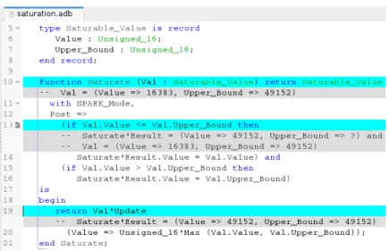
Our second example, shown in Figure 9, illustrates the handling of records. The record values are displayed in the usual Ada syntax as aggregates. If the counterexample value of a field is not known, it is displayed as a question mark. If there is more than one such field, then these fields are aggregated under the name others. On Figure 9, type Saturable_Value defined at line 5–8 contains a field Value representing the actual value and a field Upper_Bound being an up-per bound of the saturation range. The postcondition of the function Saturate is analogous to the postcondition of the procedure Saturate from Figure 8. The field Value of the returned record must contain the value of the field Value of the input record if it is in the range, otherwise it must contain the upper bound of the range. Instead of using bitwise AND, the saturation is now implemented using function Unsigned_16’Max. The counterexample shows that if Val.Value is 16383 and Val.Upper_Bound is 49152, Saturate’Result.Val is 49152. In-deed, instead of the function Unsigned_16’Max, the function Unsigned_16’Min should be used.
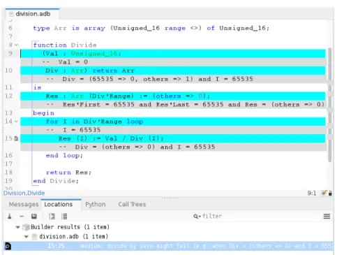
Our third example, shown in Figure 10, illustrates the handling of arrays. The function Divide takes a value Val and an array of values Div as arguments. It divides the value Val with each value in the array and returns an array with results of divisions. As shown in the counterexample, division by zero can hap-pen when some value stored in the array is zero. As for records, array values in counterexamples are displayed in Ada syntax, as array aggregates. The indices that are not relevant are summarized under the name others. For arrays with statically unknown ranges, the array range is also part of the counterexample, shown again in Ada syntax using the attributes ’First and ’Last.
Figure 9: Counterexample with a record type.
5. Experimental Evaluation
Our implementation of counterexample generation is publicly available in
Why3 0.87 and SPARK 17.0, and all later releases of Why3 and SPARK.1We
conducted an experimental evaluation in order to answer several questions: 1. Does the extra processing induced by the handling of counterexample
annotations in the tool chain result in a significant slowdown in the suc-cessfully proved VCs, or even worse decrease the provability of these VCs? 2. Are the generated counterexamples helpful for the typical user of formal
proof features of SPARK?
3. Are the counterexamples produced good ones, in the sense that they really exhibit a set of values for which the given check cannot be proved? Concerning the first question, we simply notice that on the full SPARK re-gression test-suite consisting of 1472 tests, enabling counterexample generation on all supported platforms only induces a small slowdown that is hardly sig-nificant with respect to other small variations of measurement between several runs of the same test-suite.
Concerning the second, quite informal, question, the answer based on our experience is yes. In our own practice of using SPARK, counterexamples were useful, in particular for debugging simple mistakes in annotations. Moreover, in training sessions for new users of SPARK, the presentation of counterexamples appeared to be a very useful feature for them.
1Both tool chains are free/libre and open source software (FLOSS), and available online
Figure 10: Counterexample with an array type.
The third question may seem surprising, but remember, as already said in the introduction, that due to the incompleteness of the VC generation process and also the incompleteness of the proof search by back-end solvers, our method only produces potential counterexamples. This question is especially important because in practice the back-end solver is often interrupted after a given time limit, and the counter-model given in that case is not even guaranteed to model the decidable fragment (i.e. for the quantifier-free clauses, free from non-linear arithmetic) of the proof task.
To answer the third question, we applied our implementation to a test-suite that was initially created for the Riposte tool, which was used in the previous versions of SPARK to generate counterexamples, using a completely different approach [22].
We classify the results obtained into three categories. For each VC, either the result is:
• Correct: the counterexample is truly an assignment that makes the given VC invalid.
• Wrong: the counterexample does not invalidate the VC. • Absent: there is no counterexample produced at all.
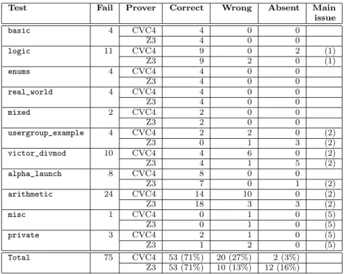
The complete results are given in Figures 11 and 12. The second column indicates the number of failing VCs in the given test, and the third indicates
Test Fail Prover Correct Wrong Absent Main issue basic 4 CVC4 4 0 0 Z3 4 0 0 logic 11 CVC4 9 0 2 (1) Z3 9 2 0 (1) enums 4 CVC4 4 0 0 Z3 4 0 0 real_world 4 CVC4 4 0 0 Z3 4 0 0 mixed 2 CVC4 2 0 0 Z3 2 0 0 usergroup_example 4 CVC4 2 2 0 (2) Z3 0 1 3 (2) victor_divmod 10 CVC4 4 6 0 (2) Z3 4 1 5 (2) alpha_launch 8 CVC4 8 0 0 Z3 7 0 1 (2) arithmetic 24 CVC4 14 10 0 (2) Z3 18 3 3 (2) misc 1 CVC4 0 1 0 (5) Z3 0 1 0 (5) private 3 CVC4 2 1 0 (5) Z3 1 2 0 (5) Total 75 CVC4 53 (71%) 20 (27%) 2 (3%) Z3 53 (71%) 10 (13%) 12 (16%) Figure 11: Results of counterexample generation on Riposte tests.
which prover was queried for a counterexample. The tests were run on both Z3 4.5.0 and CVC4 1.5 which have their own strengths and weaknesses. The next three columns indicate the number of counterexamples falling in each of the three categories above, the distinction between the Correct and Wrong cases being done by manual inspection. We analyzed the wrong or absent results and we identified the following classes of issues, which are also indicated in the last column of the table.
1. Unexpected simplification removing variables. In some simple but rare cases, a variable may disappear from a VC due to early formula simplifi-cation. For example, an expression like B and not B is replaced by false, and no counterexample value for B will be given (e.g. in example logic in Figure 11).
2. Incompleteness of the prover. In presence of undecidable logics, the coun-terexample produced may be wrong (or absent). This is expected since the prover cannot be complete in such cases. The typical case is non-linear integer arithmetic (e.g. in example arithmetic in Figure 11).
3. Implementation weakness with array initializers. The current translation of Ada array initializers to WhyML introduces an extra quantified axiom, which is difficult for the solver to instantiate adequately. This is not due to the method for generating counterexamples, but a consequence of provers’
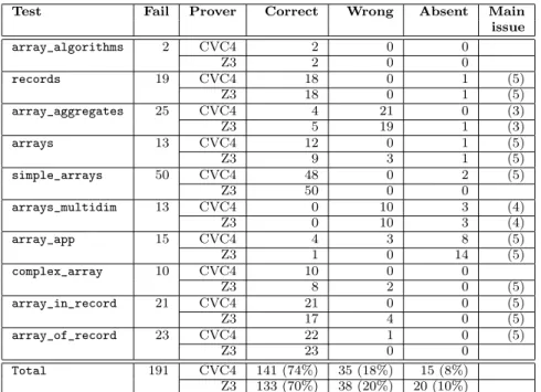
Test Fail Prover Correct Wrong Absent Main issue array_algorithms 2 CVC4 2 0 0 Z3 2 0 0 records 19 CVC4 18 0 1 (5) Z3 18 0 1 (5) array_aggregates 25 CVC4 4 21 0 (3) Z3 5 19 1 (3) arrays 13 CVC4 12 0 1 (5) Z3 9 3 1 (5) simple_arrays 50 CVC4 48 0 2 (5) Z3 50 0 0 arrays_multidim 13 CVC4 0 10 3 (4) Z3 0 10 3 (4) array_app 15 CVC4 4 3 8 (5) Z3 1 0 14 (5) complex_array 10 CVC4 10 0 0 Z3 8 2 0 (5) array_in_record 21 CVC4 21 0 0 (5) Z3 17 4 0 (5) array_of_record 23 CVC4 22 1 0 (5) Z3 23 0 0 Total 191 CVC4 141 (74%) 35 (18%) 15 (8%) Z3 133 (70%) 38 (20%) 20 (10%)
Figure 12: Results of counterexample generation on Riposte tests (arrays and records).
incompleteness in the presence of quantifiers, and we should consider an alternative simpler translation scheme to overcome that issue (e.g. in example array_aggregates in Figure 12).
4. Implementation weakness with multidimensional arrays. Specifically with multidimensional arrays (but not arrays of arrays), our current imple-mentation has some deficiencies in how it interprets the counter-model generated, and needs to be improved (e.g. in example array_multidim in Figure 12).
5. Unclassified issues. The Wrong counterexamples for which we did not identify an explanation yet fall in this default category.
The following toy example illustrates the incompleteness issue in the presence of non-linear arithmetic.
Example 15. The following Ada code attempts to check that the given number 12166397 is prime, which is incorrect (3407 × 3571).
procedure RSA (A, B: in Natural)
with Pre => A ≥ 2 and B ≥ 2
is C : Integer; begin C := 12166397; pragma Assert (A * B /= C); end RSA;
Neither CVC4 nor Z3 proves the incorrect assertion, but the counterexamples proposed are wrong or absent: respectively A = 2, B = 2 for CVC4, and no coun-terexamples for Z3. Note however that for a similar example with the smaller number 323 instead of 12166397, Z3 is able to produce the correct counterexam-ple A = 17, B = 19. This emphasizes the impredictability of results when using SMT solvers on undecidable logics.
In all, the obtained ratio of correct counterexamples to the total number of failing VCs is satisfactory: around 70%. Implementation issues identified make us confident that this ratio could be significantly improved. We discuss below other possible ways to improve the approach, beyond the remaining implemen-tation issues identified above.
6. Conclusions and Perspectives
We proposed an approach for adding support for the generation of counterex-amples in a VC generator based on a weakest-precondition calculus, making use of SMT solvers for discharging the VCs. We emphasize the importance of general features in the logic language (labels on formulas, proof task transformations) and the design of general techniques (declaration of coercion functions). Com-pared to the first version of this work [13], the technique of coercions, together with the post-processing of the counter-model produced by the back-end solver, were made more generic and robust. This solved in particular an issue with the handling of arrays identified in [13].
This approach is implemented in the Why3 environment, and exploited by its SPARK 2014 front-end for providing counterexamples to SPARK programmers in a user-friendly manner, in the development interface. The counterexample generation feature has been deployed since SPARK 16.0 distributed in 2016. Based on the feedback we got from users, in particular from new SPARK users during training sessions, we believe that counterexamples may be the most useful feature in SPARK for investigating unproved properties, along with the ability to execute contracts and assertions in tests.
6.1. Related Work
The model returned by a SAT or SMT solver on a satisfiable problem is exploited in several areas of program verification, a major case being the one of model checking, as for example in the Alloy analyzer [23] or the CBMC model checker for C programs [24].
In the case of deductive verification, generating counterexamples is not as common. The Riposte tool based on answer set programming [22] was used in the previous versions of SPARK to generate counterexamples, but only at the level of VCs without source traceability. The Isabelle proof assistant also includes a tool for generating counterexamples: the NitPick tool [25]. None of these techniques make use of a SAT or SMT solver.
In the more specific case of program verifiers using SMT solvers, the idea of instrumenting the generation of VCs originates from the old system
ESC/Modu3, that generates VCs for the Simplify solver, adding specific la-bels to determine the source location and the path of execution leading to the potential program error. The same mechanism was reused in ESC/Java [26]. The potential counterexample proposed by Simplify can be displayed to the user, but is very hard to understand because of the various encodings from the input program to the VC. More recently in 2014, a way to reinterpret the counterexample in terms of variables of the source code was designed in the OpenJML framework [3]. They use the SMT-LIB command (get-value) to get counterexample values for all sub-expressions in the original program, sup-porting values of scalar types only, and also to get values of block predicates, which they use to determine the control-flow path of the failed assertion [27]. In SPARK, it is possible to generate VCs for individual control-flow paths and display control-flow path for such VCs if they cannot be proved. In OpenJML, SMT-LIB VCs are generated directly, without using an intermediate represen-tation. On the one hand, this makes it easier to maintain a mapping between source-code variables and logical variables. On the other hand, using Why3 as intermediate language makes it possible to use the power of Why3 transforma-tions to transform a proof task to forms well suited for different provers.
Another deductive program verification framework that makes use of SMT counter-models is the Boogie Verifier Debugger [28]. Boogie is used as an inter-mediate language by Dafny [2] and VCC [29]. Boogie also has its own way of reinterpreting the counter-model, generated by its back-end prover Z3, in terms of the source code. Besides scalar values, Boogie makes it possible to display the content of dynamically allocated data structures such as objects. Unlike OpenJML, Boogie encodes locations and source variable names in the gener-ated VC, uses the SMT-LIB command (get-model) to get whole SMT-LIB counterexamples and then relies on reverse transformations to map the SMT-LIB counterexamples into the source code. On our side, we were using the (get-value) command in the previous version of this work [13], but now we use the command (get-model), because (get-value) is not powerful enough for the support of arrays.
Both OpenJML and Boogie present the counterexample in a user-friendly manner, in their respective graphical interfaces (Eclipse, Visual Studio). Their presentation is a bit different from our way of presenting the counterexample, where we give values of relevant variables inside comments at proper locations of the source code. We have no evidence that our approach is better than these other approaches in terms of quality of the generated counterexamples. We designed our approach so that it is the best fit for SPARK users.
Another recent approach for helping users in debugging their specification and code is to use some kind of symbolic execution, as is proposed by the Visual Studio dynamic debugger [30], the Verifast verifier [31] and the KeY environment [32].
6.2. Future Work
During this work, we encountered a few issues that could be addressed by authors of SMT solvers.
First, the SMT-LIB standard does not specify any rule for displaying model
values. In particular, it is not standardized how values of array types and
bit-vector types should be displayed. This forced us to implement an ad-hoc parsing in our post-processing procedure to reconstruct a counter-model from the answer of the (get-model) SMT command. This need for standardization is already known and fortunately it is likely to appear in the near future.
A second issue concerns the validity of generated counterexamples. In prin-ciple, one should query SMT solvers for models only if the answer was ‘sat’. However, for a VC generated by a program verification task, most of the time the answer is ‘unknown’ or the solver hits the time limit given. As expected, in this case the model is not guaranteed to be a true model. However, there are some cases where the model returned is trivially wrong because it is not even a model of the ground part of the goal (i.e. the terms that do not involve quan-tification). A suggestion for improvement is as follows: since the main source of incompleteness comes from the quantified hypotheses, there could be two differ-ent modes of operation, with two corresponding time limits. A first time limit, say a “soft” one, gives the time during which the solver is allowed to instantiate quantifiers as it wants. After this soft time limit is reached, a “hard” time limit should give the solver extra time to continue its search but in a specific mode where no new quantifier instantiation is performed. In this second mode, it is likely that the solver would terminate its search, and if a model is returned, it would be valid with respect to the ground part of the goal. If such modes were implemented in SMT solvers, it would be of major interest for counterexam-ple generation. This need for a soft time limit was reported on the SMT-LIB mailing list. The answers suggest that such a support is unlikely to appear in SMT solvers. A proposed work-around is to feed the solver with hypotheses of the proof task in an incremental way, so that counter-models could be queried incrementally too. We may consider implementing this approach in the future. Another technical issue is the ability to support model generation for all supported theories, including the undecidable ones such as non-linear integer arithmetic. If there is no way to be sure that the returned model would be a true one, a similar degraded mode as described above could be implemented. For example in the degraded mode non-linear parts of the formulas could be ignored.
To double-check that a counterexample produced by our technique is a true one, one may consider turning it into a test case and run the program with the given values. This is unfortunately not an easy task because of procedure calls: a procedure has a concrete semantics given by concrete execution and abstract semantics given by contracts. Since only the abstract semantics is visible to a solver, a counterexample may be true with respect to the abstract semantics, but false with respect to the concrete semantics and moreover it can happen that there is a different counterexample, not returned by the solver, true with respect to both semantics. Thus, properly combining counterexamples gener-ated by failed proof attempts and run-time verification needs to be investiggener-ated further. Recent work by Christakis et al. [33] and Petiot et al. [34] pursue such a direction.
Acknowledgements. We would like to thank David Cok, Cl´ement Fumex, Rus-tan Leino, Andrei Paskevich, Florian Schanda, as well as the anonymous re-viewers for their useful comments.
References
[1] E. W. Dijkstra, A discipline of programming, Series in Automatic Compu-tation, Prentice Hall Int., 1976.
[2] K. R. M. Leino, V. W¨ustholz, The Dafny integrated development environ-ment, in: C. Dubois, D. Giannakopoulou, D. M´ery (Eds.), Proceedings 1st Workshop on Formal Integrated Development Environment, F-IDE 2014, Grenoble, France, April 6, 2014., Vol. 149 of Electronic Proceedings in The-oretical Computer Science, 2014, pp. 3–15. doi:10.4204/EPTCS.149.2. [3] D. R. Cok, OpenJML: Software verification for Java 7 using JML,
Open-JDK, and Eclipse, in: C. Dubois, D. Giannakopoulou, D. M´ery (Eds.),
Proceedings 1st Workshop on Formal Integrated Development Environ-ment, Vol. 149 of EPTCS, 2014, pp. 79–92.
[4] F. Bobot, J.-C. Filliˆatre, C. March´e, A. Paskevich, Let’s verify this with Why3, International Journal on Software Tools for Technology Trans-fer (STTT) 17 (6) (2015) 709–727, see also http://toccata.lri.fr/ gallery/fm2012comp.en.html. doi:10.1007/s10009-014-0314-5. [5] F. Bobot, S. Conchon, E. Contejean, M. Iguernelala, S. Lescuyer, A.
Meb-sout, The Alt-Ergo automated theorem prover, http://alt-ergo.lri.fr/ (2008).
[6] C. Barrett, C. L. Conway, M. Deters, L. Hadarean, D. Jovanovi´c, T. King,
A. Reynolds, C. Tinelli, CVC4, in: Proceedings of the 23rd
interna-tional conference on Computer aided verification, CAV’11, Springer-Verlag, Berlin, Heidelberg, 2011, pp. 171–177.
URL http://dl.acm.org/citation.cfm?id=2032305.2032319
[7] L. de Moura, N. Bjørner, Z3, an efficient SMT solver, in: TACAS, Vol. 4963 of Lecture Notes in Computer Science, Springer, 2008, pp. 337–340. [8] J.-C. Filliˆatre, A. Paskevich, Why3 — where programs meet provers, in:
M. Felleisen, P. Gardner (Eds.), Proceedings of the 22nd European Sym-posium on Programming, Vol. 7792 of Lecture Notes in Computer Science, Springer, 2013, pp. 125–128.
[9] J.-C. Filliˆatre, C. March´e, The Why/Krakatoa/Caduceus platform for de-ductive program verification, in: W. Damm, H. Hermanns (Eds.), 19th International Conference on Computer Aided Verification, Vol. 4590 of Lecture Notes in Computer Science, Springer, Berlin, Germany, 2007, pp. 173–177.
[10] N. Kosmatov, C. March´e, Y. Moy, J. Signoles, Static versus dynamic veri-fication in Why3, Frama-C and SPARK 2014, in: T. Margaria, B. Steffen (Eds.), 7th International Symposium on Leveraging Applications of Formal Methods, Verification and Validation (ISoLA), Vol. 9952 of Lecture Notes in Computer Science, Springer, Corfu, Greece, 2016, pp. 461–478.
[11] F. Bobot, J.-C. Filliˆatre, C. March´e, A. Paskevich, Why3: Shepherd your herd of provers, in: Boogie 2011: First International Workshop on In-termediate Verification Languages, Wroc law, Poland, 2011, pp. 53–64, https://hal.inria.fr/hal-00790310.
[12] M. Barnett, R. DeLine, B. Jacobs, B.-Y. E. Chang, K. R. M. Leino, Boo-gie: A Modular Reusable Verifier for Object-Oriented Programs, in: F. S. de Boer, M. M. Bonsangue, S. Graf, W.-P. de Roever (Eds.), Formal Meth-ods for Components and Objects: 4th International Symposium, Vol. 4111 of Lecture Notes in Computer Science, 2005, pp. 364–387.
[13] D. Hauzar, C. March´e, Y. Moy, Counterexamples from proof failures in
SPARK, in: Software Engineering and Formal Methods, 2016, pp. 215– 233.
[14] C. Flanagan, J. B. Saxe, Avoiding exponential explosion: Generating com-pact verification conditions, in: Principles Of Programming Languages, ACM, 2001, pp. 193–205.
[15] K. R. M. Leino, Efficient weakest preconditions, Information Processing Letters 93 (6) (2005) 281–288.
[16] C. Belo Louren¸co, M. J. Frade, J. Sousa Pinto, Formalizing
single-assignment program verification: An adaptation-complete approach, in: P. Thiemann (Ed.), 25th European Symposium on Programming, Springer, 2016, pp. 41–67. doi:10.1007/978-3-662-49498-1_3.
URL http://dx.doi.org/10.1007/978-3-662-49498-1_3
[17] C. Barrett, A. Stump, C. Tinelli, The SMT-LIB Standard: Version 2.0, in: A. Gupta, D. Kroening (Eds.), Proceedings of the 8th International Workshop on Satisfiability Modulo Theories (Edinburgh, England), 2010. [18] C. Dross, S. Conchon, J. Kanig, A. Paskevich, Adding decision procedures
to SMT solvers using axioms with triggers, Journal of Automated Reason-ing 56 (4) (2016) 387–457.
[19] J. Barnes, Programming in Ada 2012, Cambridge University Press, 2014. [20] J. W. McCormick, P. C. Chapin, Building High Integrity Applications with
SPARK, Cambridge University Press, 2015.
[21] R. Chapman, F. Schanda, Are we there yet? 20 years of industrial theorem proving with SPARK, in: G. Klein, R. Gamboa (Eds.), Interactive Theorem Proving - 5th International Conference, ITP 2014, Held as Part of the
Vienna Summer of Logic, VSL 2014, Vienna, Austria, July 14-17, 2014. Proceedings, Vol. 8558 of Lecture Notes in Computer Science, Springer, 2014, pp. 17–26. doi:10.1007/978-3-319-08970-6_2.
[22] F. Schanda, M. Brain, Using Answer Set Programming in the Development of Verified Software, in: Technical Communications of the 28th Int. Conf. on Logic Programming, Vol. 17 of LIPIcs, Leibniz-Zentrum fuer Informatik, 2012, pp. 72–85. doi:http://dx.doi.org/10.4230/LIPIcs.ICLP.2012. 72.
[23] Alloy, http://alloy.mit.edu/.
[24] A. Groce, D. Kroening, F. Lerda, Understanding counterexamples with explain, in: R. Alur, D. Peled (Eds.), CAV, Vol. 3114 of Lecture Notes in Computer Science, Springer, 2004, pp. 453–456.
[25] J. C. Blanchette, T. Nipkow, Nitpick: A counterexample generator for higher-order logic based on a relational model finder, in: M. Kaufmann, L. C. Paulson (Eds.), Interactive Theorem Proving, First International Conference, Vol. 6172 of Lecture Notes in Computer Science, Springer, 2010, pp. 131–146.
[26] K. R. M. Leino, T. Millstein, J. B. Saxe, Generating error traces from verification-condition counterexamples, Science of Computer Programming 55 (13) (2005) 209 – 226. doi:http://dx.doi.org/10.1016/j.scico. 2004.05.016.
[27] D. R. Cok, Improved usability and performance of SMT solvers for debug-ging specifications, Int. Journal on Software Tools for Technology Transfer 12 (6) (2010) 467–481. doi:10.1007/s10009-010-0138-x.
[28] C. Le Goues, K. R. M. Leino, M. Moskal, The Boogie Verification Debug-ger, in: G. Barthe, A. Pardo, G. Schneider (Eds.), Software Engineering and Formal Methods - 9th International Conference, (SEFM), Vol. 7041 of Lecture Notes in Computer Science, Springer, 2011, pp. 407–414.
[29] E. Cohen, M. Dahlweid, M. Hillebrand, D. Leinenbach, M. Moskal, T. San-ten, W. Schulte, S. Tobies, VCC: A practical system for verifying concurrent C, in: Theorem Proving in Higher Order Logics (TPHOLs), Vol. 5674 of Lecture Notes in Computer Science, Springer, 2009.
[30] P. M¨uller, J. N. Ruskiewicz, Using debuggers to understand failed verifi-cation attempts, in: M. J. Butler, W. Schulte (Eds.), 17th International Symposium on Formal Methods, Vol. 6664 of Lecture Notes in Computer Science, Springer, 2011, pp. 73–87.
[31] B. Jacobs, J. Smans, P. Philippaerts, F. Vogels, W. Penninckx, F. Piessens, VeriFast: A powerful, sound, predictable, fast verifier for C and Java, in:
M. G. Bobaru, K. Havelund, G. J. Holzmann, R. Joshi (Eds.), NASA For-mal Methods, Vol. 6617 of Lecture Notes in Computer Science, Springer, 2011, pp. 41–55.
[32] M. Hentschel, R. H¨ahnle, R. Bubel, Deductive Software Verification — The KeY Book, Springer, 2016, Ch. Debugging and Visualization, pp. 383–413. doi:10.1007/978-3-319-49812-6_11.
URL http://dx.doi.org/10.1007/978-3-319-49812-6_11
[33] M. Christakis, K. R. M. Leino, P. M¨uller, V. W¨ustholz, Integrated environ-ment for diagnosing verification errors, in: 22nd International Conference on Tools and Algorithms for the Construction and Analysis of Systems (TACAS’16), Springer, 2016, pp. 424–441.
[34] G. Petiot, N. Kosmatov, B. Botella, A. Giorgetti, J. Julliand, Your proof fails? testing helps to find the reason, in: Tests and Proofs - 10th In-ternational Conference, Vol. 9762 of Lecture Notes in Computer Science, Springer, 2016, pp. 130–150.