Smoothing PLLs for QAM Dynamical Phase Estimation

(1)

HAL Id: hal-01224236

https://hal-ensta-paris.archives-ouvertes.fr//hal-01224236

Submitted on 4 Dec 2015

HAL is a multi-disciplinary open access

archive for the deposit and dissemination of

sci-entific research documents, whether they are

pub-lished or not. The documents may come from

teaching and research institutions in France or

abroad, or from public or private research centers.

L’archive ouverte pluridisciplinaire HAL, est

destinée au dépôt et à la diffusion de documents

scientifiques de niveau recherche, publiés ou non,

émanant des établissements d’enseignement et de

recherche français ou étrangers, des laboratoires

publics ou privés.

Smoothing PLLs for QAM Dynamical Phase Estimation

Jianxiao Yang, Benoit Geller, Cedric Herzet, Jean-Marc Brossier

To cite this version:

Jianxiao Yang, Benoit Geller, Cedric Herzet, Jean-Marc Brossier. Smoothing PLLs for QAM

Dynam-ical Phase Estimation. ICC 2009 - IEEE International Conference on Communications, Jun 2009,

Dresden, Germany. pp.100, �10.1109/ICC.2009.5199465�. �hal-01224236�

(2)

Abstract—This paper presents a near-optimum, low-complexity,

fixed-interval smoothing algorithm that approaches the performance of an optimal smoother for the price of two low-complexity sequential estimators (two PLLs). The proposed Smoothing PLL (S-PLL) algorithm is easy to implement and fits the Cramer-Rao bounds over a wide range of signal-to-noise ratios. Moreover we show that, compared to the conventional forward loop, the proposed scheme allows to have a large gain of several dBs and is able to track frequency offsets.

Keywords-Dynamical Phase Estimation; Phase-Locked Loop

(PLL); QAM; Smoothing Algorithm.

I. 0BINTRODUCTION

Due to the increasing requirements of modern

communication systems to face the physical channel (low signal-to-noise ratio, high data rates), phase estimation is more challenging than ever before. Since phase errors rapidly degrade the overall performance of communication systems, synchronization has recently become one of the most challenging tasks that a digital receiver has to cope with.

Noels et al [1],[2]X derived a maximum likelihood (ML)

algorithm for the problem of constant phase estimation, and then applied a first-order and a second order phase-locked loop (PLL) based algorithm for the coded BPSK and QPSK dynamical phase estimation. The corresponding performances are limited both by the on-line bound and by a non-zero phase MSE floor. On the contrary, this paper deals with the non data aided (NDA) estimation of a time-varying phase and proposes an off-line Smoothing PLL (S-PLL) algorithm. To assess the performance of such algorithms, Bayesian and hybrid Cramér-Rao Bounds (BCRB and HCRB) associated to this dynamical phase synchronization problem have already been considered in some recent contributions X[3]XX-[6]X and clearly show the

superiority of the off-line scenario [7].

In practice, on-line estimators are often considered for complexity considerations. Among the famous algorithms, phase-locked loops are recognized low-cost devices for on-line estimation and have been integrated in many existing systems

X[8]X-X[11]X. Despite a poor transient behaviour, their excellent

asymptotic (i.e. tracking) characteristic makes them a reference from the performance-complexity trade-off point of view. The

1_{This work was partially funded by the ANR LURGA program.} J. Yang is with SATIE, ENS Cachan,

(e-mail: shawn.yang@satie.ens-cachan.fr)

B. Geller is with LEI, ENSTA ParisTech (e-mail: geller@ensta.fr) C. Herzet is with IRISA, INRIA Rennes (e-mail: cedric.herzet@irisa.fr) J.M. Brossier is with GIPSA, Grenoble INP,

(e-mail: jean-marc.brossier@gipsa-lab.inpg.fr)

poor transient behaviour has now been handled by several

authors for many years (see e.g. X[12]X). The good performance

of such PLLs can even be improved at low SNRs within the turbo-receiver framework (see e.g. X[1],XX[2]XX,[13]X) but this paper

is definitely not concerned about the code-aided framework.

X[14]X proposed a CA belief-propagation (BP) algorithm for the

BPSK dynamical phase estimation but the computation complexity of the proposed BP algorithm is rather high. This paper is concerned with a very simple synchronizing scheme for any QAM modulated signal which is able to operate near the off-line time-varying phase bounds. To our knowledge, it was first proposed without any justification and without any performance evaluation in X[15]X-X[17]X; contrarily to X[1]XX,[2]X, it

takes advantage of averaging two phase trajectories provided by two PLLs, so that this S-PLL algorithm is able to have such a near off-line Cramér-Rao bound performance.

The rest of the paper is organized as follows. In section XIIX,

we give the system model. In section XIIIX, we derive from the

MAP estimation theory the proposed algorithm where the smoothing effect is achieved through two PLLs working in opposite time directions. Finally in section XIVX, we present the

simulation results before giving some conclusions.

II. 1BSYSTEM MODEL

We consider the transmission of a complex-valued QAM

modulated sequence  1, , 

T

c c



c  (ckSM) over an AWGN

channel affected by some carrier phase offsets stacked in a

vector  1, , 

T

 



θ  . Assuming that the timing recovery is

perfect without any inter-symbol interference (ISI), the

sampled baseband signal  1, , 

T y y  y  is written as: , k j k k k y c e n (1)

where ck, k and nk are respectively the i.i.d. k- t h unknown

transmitted constellation symbol ( p c k 1 M ), the residual

phase distortion and the zero mean complex-valued circular

Gaussian noise with known variance 2

n

 . We suppose that the

system operates in a non-data aided (NDA) mode. Hence, the

conditional probability based on the known phase k is:

        M 2 2 2 1 | | , e x p , , M k k k k k k k k k k k k c n n c y p y  p y  c p c c y                     S ， (2) where  





2 2 2 R e , , e x p k j k k k k k k n c y c e c y                   .

In practice, due to the rapid variant channel and the imperfections of the functional blocks before the phase

Smoothing PLLs for QAM Dynamical Phase Estimation

J. Yang，B. Geller, C. Herzet, and J.M. Brossier

F 1

(3)

estimation, the residual phase distortion can be modeled efficiently by a Brownian motion. The corresponding phase model is:

1 ,

k k wk

     (3)

where k is the unknown phase offset at time k ,  is the

unknown constant frequency offset (linear drift), wk is a

real-valued white Gaussian noise with zero mean and variance 2

w

 . This model is commonly used X[18]X-X[21]X in order to describe

the behavior of practical oscillators for which the frequency is randomly perturbed. Based on (3), the corresponding conditional probability can be expressed as:

    2 1 1 2 1 | , e x p . 2 2 k k k k w w p             _ _           (4)

III. 2BRATIONALE FOR AFORWARD /BACKWARD APPROACH

BY MAPESTIMATION THEORY

In the MAP estimation approach, one classically chooses ˆθ

to maximize the posterior pdf X[22]:

     

ˆ __{a r g m a x}_p _| __{a r g m a x}__ln_p _| __ln_p _

 

θ θ

θ θ y y θ θ (5)

Based on the model described by (2) and (4), the joint pdf of the observations and the parameters can be written as:

                      1 M M 1 1 1 1 2 1 2 1 1 1 1 1 2 2 2 2 1 2 2 2 , , | | | | | , 1 1 e x p , , 2 e x p , , 2 k k k k k k c n w n k k k k k k c k n w p p p p p y p y p y p c y M y c y                                               _ _  _{ }  _                             S S y θ y θ θ      (6)

It is easy to obtain for any k the first derivative of

  ln_p y θ, , _:           1 M 1 M 1 1 1 1 1 2 1 2 1 1 1 1 1 , , ln , , ln , , c w c c y p p c y                 _ _  _ _            S S y θ ,         M M 1 1 2 , , ln , , 2 , , k k k k k c k k k k k k k k w c c y p c y                 _            S S y θ for 2k   1,         M M 1 2 , , ln , , , , , c w c c y p c y                            _            S S y θ (7) where     2





, , 2 , , Im k k k k j k k k k k k n c y c y y c e             . Looking for

the MAP estimator implies that one must set the first

derivative ln  , ,  k p    _ _  y θ equal to 0, so that:       1 M 1 M 1 1 1 1 2 1 2 1 2 1 1 1 1 , , ln , , , c w w c c y p c y                   _ _         S S         M M M M 2 2 1 1 , , , , 1 2 2 , , 2 , , k k k k k k k k k k c k c k w w k k k k k k k k k c c c y c y c y c y                                         _   _  _ _ _ _           S S S S for 2k   1,     M M 2 1 , , . , , c w c c y c y                               S S (8) Rewrite     M M , , , , k k k k k c k k k k c c y c y            S S

as below in order to get the

physical meaning of the term:

   













   





M M M M M M 2 2 2 2 2 2 2 R e 2 Im , , _{e x p} , , _{2 R e} e x p | , 2 Im . | , k k k k k k k k k k j j k k k k k k k k c n n c k j k k k _k _k _k c c n k k k j k k c n k k k c c y c e y c e c y c y _c _{y c e} p y c y c e p y c                            _ _           _ _   __ _ _              S S S S S S   (9)

One can then recognize that the factor Im



jk



k k

y c e  is just

the classical hard decision phase detector output based on the

decision ck, while the factor

    M | , | , k k k k k k k c p y c p y c     S   is exactly the a

posteriori probability (APP) P rc_k|y_k,_k in the NDA scenario.

Thus the term

    M M , , , , k k k k k c k k k k c c y c y            S S

can be interpreted as the soft

decision phase detector output. (9) can then be written as:

 





     





 





1 1 M M 2 1 2 1 2 2 1 1 1 11 1 2 1 2 ln 2 P r | , Im , 1 f o r 2 1, 2 2 P r | , Im , j w w c n F B k k k j w c n p c y y c e k c y y c e                                       _ _                     S S      (10)

(4)

where    





   





M M 2 1 2 2 1 2 P r | , Im , P r | , Im . k k k k F w j k k k k k k k c n B w j k k k k k k k c n c y y c e c y y c e                           _     S S   (11) Furthermore in (11),  F k  and  B k

 can be regarded as

soft-decision based first-order PLL outputs which are respectively updated in the increasing (Forward) and decreasing (Backward) time directions. The physical meaning of (9) can thus be summarized as following; assuming that we do not have any a priori information about the initial phase 1 (i.e.

 1 1 ln 0 p    _   

 ), the estimator is just estimated from 2 with a

backward recursion PLL; for the last position k  element,

the estimator is estimated from  1with a forward PLL; and

in the general case ( 1k   ), the phase estimator is

estimated both from the previous and the following samples, i.e. as the average of a forward and of a backward PLL. Since in practice it is impossible to get the actual phase valuek

before estimating it, we replace in (11) the true phase k by

the forward estimate  1

ˆF k

 _ and the backward estimate  1

ˆ B k  _ :    

_

 

_

 





   

_

 

_



 



1 M 1 M 2 ˆ 1 2 1 2 ˆ 1 2 1 ˆ ˆ _{P r} _| _,ˆ _Im _, ˆ ˆ _{P r} _| _,ˆ _Im _. F k k B k k F F w F j k k k k k k k c n B B w B j k k k k k k k c n c y y c e c y y c e                               _     S S   (12)

From (8) the “Forward / Backward” (F/B) estimator can thus be written as:    

_

 

_

 





     





   

_

 

_

 





2 1 M 1 M 2 ˆ / 1 2 2 1 1 2 1 1 / 2 ˆ / 1 2 1 2 ˆ ˆ ˆ _{P r} _| _,ˆ _Im _, 1 ˆ ˆ ˆ _{f o r 2} _1, 2 2 ˆ ˆ ˆ _{P r} _| _,ˆ _Im _. B F F B B w B j c n F B F B k k k F B F w F j c n c y y c e k c y y c e                                                           S S (13)

Note that this structure is similar to that of the Kalman smoother valid for linear Gaussian problems. The name “Forward / Backward” stems from the fact that the off-line phase estimation is just the average of a classical (Forward) phase-locked loop and of a Backward phase-locked loop working in the reverse time direction and that can be initialized at the end of the forward PLL. This process can then be iterated, i.e. the estimation error at the end of the previous backward loop can be further used as the estimation error at the beginning of the next forward recursion, and several forward and backward recursions can sequentially be proceeded. We call this process in the sequel as “multiple forward / backward”. Restricted by the paper size, we shall give further analysis of the proposed algorithm at the oral presentation.

IV. 3BSIMULATION AND DISCUSSION

In a practical system, a frame header can be used and one could take advantage of it to get rid of the phase ambiguities. In our simulations, we thus assume that the phase ambiguity problem is solved. We evaluate the MSEs in the centre position

of the block after 3 F/B iterations over 5

1 0 Monte-Carlo trials.

The block length  for BPSK and QPSK is 60, and is 800 for

the 16QAM constellation. We use the following notations in the figures of the present paragraph. “Forward (Sim)” means that the simulation MSE is measured after one (on-line) forward estimation without any backward estimation. The “Forward / Backward (Sim)” means that the MSE of the F/B estimation is measured after three (off-line) F/B iterations.

A. 5BPerformance with no linear drift

Since all the parameters are random, we compare the estimation MSE of the “Forward (Sim)” (resp. “Forward / Backward” (Sim)) with the on-line BCRB (resp. the off-line

BCRB) X[3],[5],[6], on Fig. 1 to Fig. 3 for different

constellations. 0 5 10 15 20 25 30 -35 -30 -25 -20 -15 -10 -5 SNR (dB) M S E ( d B ) _w2

= 0.02rad2,  = 0rad, Iteration = 3

Forward (Sim) Forward / Backward (Sim) NDA BCRB On-Line NDA BCRB Off-Line DA BCRB On-Line DA BCRB Off-Line

Fig. 1 BPSK MSEs and BCRBs versus SNR

At high SNR, we notice that the forward MSE and the F/B MSE curves logically merge. In this case the observations are reliable enough to only take into account the present observation ykin order to estimatek; this is why the off-line

BCRBs (corresponding to the F/B MSE) converge to the on-line BCRBs (corresponding to the forward MSE), and this is also why the NDA bounds converge to the DA bounds. As the a priori distribution of θ then has very little influence, the Bayesian problem tends to a deterministic phase estimation problem where we estimate independent observations.

In more realistic mid-range SNRs, the F/B performance is definitely superior to the forward only recursion and the maximum difference is 3dB. In this range of SNRs, the a priori knowledge on θ plays a very important role in the phase estimation and this is why there is a larger difference

(5)

between the F/B and forward recursions compared to higher and lower SNR range.

Finally, at low SNRs, because of the decision error, the MSE increases rapidly and the non-data-aided (NDA) BCRBs do not coincide anymore with the DA BCRBs. However, generally, the performance gain using a data-aided scenario is relatively low compared to the performance difference between the off-line and the on-line scenarios, and logically, when comparing with the forward recursion, there is still an appreciable gain in favor of the F/B recursion.

5 10 15 20 25 30 -35 -30 -25 -20 -15 SNR (dB) M S E ( d B ) _w2

Forward (Sim) Forward / Backward (Sim) NDA BCRB On-Line NDA BCRB Off-Line DA BCRB On-Line DA BCRB Off-Line

Fig. 2 QPSK MSEs and BCRBs versus SNR

14 16 18 20 22 24 26 28 30 32 34 -40 -35 -30 -25 SNR (dB) M S E ( d B ) _w2

Forward (Sim) Forward / Backward (Sim) NDA BCRB On-Line NDA HCRB Off-Line DA BCRB On-Line DA BCRB Off-Line

Fig. 3 16QAM MSEs and BCRBs versus SNR

B. 6BPerformance with a linear drift

Since the parameters contain both some random parameters

k

 and a deterministic linear drift , we compare the MSEs to

HCRBs of interest X[4]-[6] for different constellations on Fig. 4

to Fig. 6.

At high SNR, the off-line HCRB coincides with the on-line HCRB, and so are the corresponding MSEs. Because in this range of SNR, the information provided by the observation is

dominating over the a priori knowledge on θ,theobservation

k

y isself-sufficienttoestimatek andtheerroron does not

disturbtheestimationperformanceonk.

0 5 10 15 20 25 30 -35 -30 -25 -20 -15 -10 SNR (dB) M S E ( d B ) _w2

= 0.001rad2,  = 0.03rad, Iteration = 3

Forward (Sim) Forward / Backward (Sim) NDA HCRB On-Line NDA HCRB Off-Line DA HCRB On-Line DA HCRB Off-Line

Fig. 4 BPSK MSEs and HCRBs versus SNR

10 15 20 25 30 -35 -30 -25 -20 -15 SNR (dB) M S E ( d B ) _w2

Fig. 5 QPSK MSEs and HCRBs versus SNR

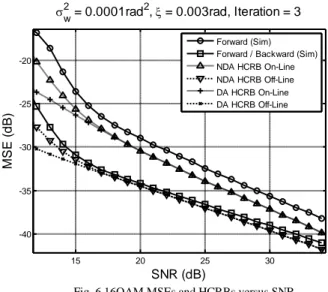
At mid-range SNRs, there is not enough information

provided by yk to estimate the phase and one can take

advantage of the a priori knowledge on θ (see the difference between the on-line and the off-line BCRBs). The F/B estimation is definitely superior (up to 5 dB on Fig. 4) to the

forward MSE not only thanks to the a priori knowledge onθ;

this superiority also comes from the fact that the F/B scheme

remains unbiased contrarily to the forward 1st order loop which

suffers from the high linear drift as the corresponding MSE does not coincide anymore with the on-line HCRB.

At low SNRs, there is still an advantage for the F/B recursion; however the F/B performance of Fig. 4 deteriorates rapidly, because in practice the F/B recursion is made out of two unidirectional loops, and these loops are not able to operate

(6)

anymore as wanted with the considered large linear drift. This phenomenon is attenuated with a smaller linear drift (see Fig. 6) or if we had replaced our simple first order PLL components by other component loops such as second order PLLs.

15 20 25 30 -40 -35 -30 -25 -20 SNR (dB) M S E ( d B ) _w2

Fig. 6 16QAM MSEs and HCRBs versus SNR

C. 5BAlgorithm complexity analysis

The classical on-line PLL has a very low gradient-like complexity and has been employed in real systems for several decades. The complexity price for the off-line improvement is only two times that of the on-line algorithm as we combine two elementary PLLs. In addition, three forward-backward needs to be proceeded which both involves a very reasonable delay and the memorization of K symbols and of 2K phase values.

V. 4BCONCLUSION

In this paper, we presented a near-optimum smoothing phase locked loop (S-PLL) algorithm made out of two very simple first order PLLs. The performance of the S-PLL algorithm does not suffer from the poor transient behavior even with a small number of observations. The proposed scheme provides a gain of several dBs over a forward only on-line algorithm and its performance is near the Cramer-Rao bounds of interest. Finally it is very easy to implement and should be very useful in practice.

7BREFERENCES

[1] N. Noels, H. Steendam and M. Moeneclaey, "Performance Analysis of ML-Based Feedback Carrier Phase Synchronizers for Coded Signals,"

IEEE Transactions on Signal Processing, Vol. 55, pp. 1129-1136,

March 2007.

[2] N. Noels, H. Steendam, M. Moeneclaey, "Effectiveness Study of Code-Aided and Non-Code-Code-Aided ML-Based Feedback Phase Synchronizers,"

Proc. IEEE Inter. Conf. on Commun. 2006, ICC'06, Istanbul, Turkey,

June 11-15, 2006.

[3] S. Bay, C. Herzet, J.P. Barbot, J. M. Brossier, and B. Geller, "Analytic and Asymptotic Analysis of Bayesian Cramér–Rao Bound for Dynamical Phase Offset Estimation," IEEE Transactions on Signal

Processing, vol. 56, pp. 61-70, Jan. 2008.

[4] S. Bay, B. Geller, A. Renaux, J.P. Barbot, and J.M. Brossier, “On the Hybrid Cramer-Rao bound and its application to dynamical phase estimation,” IEEE Signal Processing Letters, vol. 15, pp. 453-456, 2008. [5] J. Yang, B. Geller, and A. Wei, “Bayesian and Hybrid Cramer-Rao Bounds for QAM Dynamical Phase Estimation,” in Proc. IEEE Signal

Processing, ICASSP'09, Taipei, 19-24 April 2009.

[6] J. Yang, B. Geller, and A. Wei, “Approximate Expressions for Cramer-Rao Bounds of Code Aided QAM Dynamical Phase Estimation,”in

Proc. IEEE Inter. Conf. on Commun. 2009, ICC'09, Dresden, 14-18 June

2009.

[7] J. Yang and B. Geller, “Near-optimum Low-Complexity Smoothing Loops for Dynamical Phase Estimation,” accepted by IEEE Trans.

Signal Processing.

[8] M. Simon, W. Lindsey, "Optimum Performance of Suppressed Carrier Receivers with Costas Loop Tracking, " IEEE Trans. on Commun. vol. 25, no.2, pp. 215-227, Feb. 1977.

[9] R. E. Best, Phase-Locked Loops: Design, Simulation, and Applications, 4th ed., McGraw-Hill, 2003..

[10] F.M. Gardner, Phaselock Techniques, 3rd_{ed., Wiley-Interscience, 2005.} [11] J.M. Brossier, Signal & Communication, Hermès, 1997.

[12] M.-L. Alberi, R.A. Casas, I. Fijalkow, and C.R. Jr. Johnson, "Looping LMS versus fast least squares algorithms: who gets there first?" 2nd IEEE Workshop on Signal Processing Advances in Wireless Commun.,

SPAWC 1999.

[13] L. Zhang and A. Burr, "Iterative Carrier Phase Recovery suited for Turbo-Coded systems," IEEE Trans. on Wireless Commun., vol. 3, No. 6, pp. 2267-2276, Nov. 2004.

[14] G. Colavolpe, A. Barbieri, and G. Caire, "Algorithms for iterative decoding in the presence of strong phase noise," IEEE Journal on

Selected Areas in Communications, Vol. 23, pp. 1748 – 1757, Sept. 2005.

[15] J.M. Brossier, F. Lehmann, Procédé d'estimation de la phase dans un système de communication numérique et boucle à verrouillage de phase. French patent FR20020012900, pended on the 17th_{oct. 2002.} International extension WO2004036753 on the 29th_{april 2004. Phase} Estimation Method in a Digital and Phase Locked Loop Communication System. Patent US 2006/0187894 A1. Publication date: Aug. 24, 2006. [16] B. Geller, J.P. Barbot, J.M. Brossier, and C. Vanstraceele, Procédé

d'estimation de la phase et du gain de données d'observation transmises sur un canal de transmission en modulation QAM. French patent 04P0441, pended on the 20th_{sept. 2004. Method for estimating the phase} of observation data transmitted over a QAM-modulated transmission channel. International extension PCT Fr 2005/02301, WCT 2006/032768 on the 30th_{march 2006.}

[17] B. Geller, “Contribution à l’étude des systèmes de communications numériques,” Chap. 3, Accreditation to Supervize Research (HDR) University of Paris, Dec. 2004.

[18] P.O. Amblard, J.M. Brossier, and E. Moisan, “Phase tracking: what do we gain from optimality? Particle filtering versus phase-locked loops,”

Signal Processing, vol. 83, pp. 151–167, Oct. 2003.

[19] J. A. McNeill, Jitter in ring oscillators, Ph.D. dissertation, Boston University, 1994.

[20] A. Demir, A. Mehrotra, and J. Roychowdhury, “Phase noise in oscillators: a unifying theory and numerical methods for characterization,” IEEE Trans. Circuits Syst. I, vol. 47, pp. 655–674, May 2000.

[21] ETSI TR 102 376, Digital Video Broadcasting (DVB) User guidelines

for the second generation system for Broadcasting, Interactive Services, News Gathering and other broadband satellite application (DVB-S2),

v1.1.1, Feb, 2005.

[22] S. M. Kay, Fundamentals of statistical signal processing: estimation