The Impact of Infrastructure Investments on Income Inequality: Evidence from US States

HAL Id: halshs-02736095

https://halshs.archives-ouvertes.fr/halshs-02736095v2

Preprint submitted on 21 Sep 2020

HAL is a multi-disciplinary open access

archive for the deposit and dissemination of

sci-entific research documents, whether they are

pub-lished or not. The documents may come from

teaching and research institutions in France or

abroad, or from public or private research centers.

L’archive ouverte pluridisciplinaire HAL, est

destinée au dépôt et à la diffusion de documents

scientifiques de niveau recherche, publiés ou non,

émanant des établissements d’enseignement et de

recherche français ou étrangers, des laboratoires

publics ou privés.

The Impact of Infrastructure Investments on Income

Inequality: Evidence from US States

Emma Hooper, Sanjay Peters, Patrick Pintus

To cite this version:

Emma Hooper, Sanjay Peters, Patrick Pintus. The Impact of Infrastructure Investments on Income

Inequality: Evidence from US States. 2020. �halshs-02736095v2�

Working Papers / Documents de travail

The Impact of Infrastructure Investments on Income

Inequality: Evidence from US States

Emma Hooper

Sanjay Peters

Patrick A. Pintus

The Impact of Infrastructure Investments on

Income Inequality: Evidence from US States

∗

Emma Hooper

Sanjay Peters

Patrick A. Pintus

September 9, 2020

Abstract: Our analysis of US state-level data on an annual frequency, from 1976 to 2008, sheds new light on a plausible causal link between infrastructure investments, namely public spending on highways, and income inequality. This causal relationship is drawn out by using the number of seats in the US House of Representatives Committee on Appropriations (HRCA) as an instrument to identify quasi-random variations in state-level spending on highways. An exogenous pattern which emerges when a state gains an additional member to the HRCA is that it is allocated with new federal grants. This increase in federal transfers for infrastructure financing results in slashing of expenditures on highways and a crowding-out effect of federal funding for state investments on highways. Spending cuts on highways produced by a new HRCA member being attained by a state can unwittingly cause income inequality to rise over a short two-year time horizon. Similar challenges with decentralized development to finance infrastructure via federal transfers to state and sub-national governments may be encountered by other industrially advanced, emerging and low-income developing economies. US data over the mentioned period reveal a strong positive correlation with state spending on highways and wages paid for construction jobs. Suggestive evidence indicates that the construction sector also plays an important role in the transmission channel from a rise in state spending on highways to lowering income inequality, albeit during specific intervals, as opposed to on a long-term basis.

JEL Classification Numbers: C23, D31, H72, O51

Keywords: Public Infrastructure, Highways, Income Inequality, US State Panel Data, Instrument Variable ∗_{This paper supersedes a previous version entitled “The Causal Effect of Infrastructure Investments on Income} Inequality: Evidence from US States”. The authors are grateful for referee feedback and especially to Philippe Aghion and Antonin Bergeaud for kindly sharing their dataset on US states as well as for extremely useful discussions, Simon Ray for highly valuable input at early stages of the project, Gilles Duranton, Jonathan Ostry and Juan Gabriel Rodriguez for very helpful comments and suggestions, Carl Barrick, Dave Donaldson, Martin Guzman, Juan Antonio Montecino, Estelle Sommeiller, Matt Turner, Natacha Valla and participants at the European Investment Bank, 2017 RIDGE workshop on Macroeconomics and Development at Universidad de Buenos Aires, 2018 AFSE conference, 2018 Infrastructure, Growth and Development conference, University of Lausanne, CREM, 2019 ITEA conference, 2019 Inequality and Opportunities Madrid workshop, CERDI for very useful feedback. This work was supported by French National Research Agency Grants ANR-17-EURE-0020.

†_{Aix-Marseille Univ., CNRS, AMSE. Email: emmahooper@hotmail.fr.} ‡_{Columbia University. Email: sanjay.peters@gmail.com.}

§_{Aix-Marseille Univ., CNRS, AMSE. Email: patrick.pintus@univ-amu.fr.}

1

Introduction

Long-term investments in infrastructure are increasingly at the center of many scholarly discussions, debates and policy initiatives worldwide. Many global institutions are closely examining whether countries are able to achieve long term sustainable growth through increasing public spending on infrastructure. In developed economies, one of the main objectives to reverse a much feared “secular stagnation” is through better maintenance of existing public goods, for example by, ascribing greater importance to smart and resilient infrastructure1, by investing in infrastructure that fosters innovation and which at the same time also protects the environment. In many low-income developing countries, on the other hand, electrification, the construction of public hospitals and railways are almost always debt financed. This pattern of increased spending on social infrastructure often occurs during national election campaigns, and features prominently across many Africa countries. Additionally, investment in infrastructure is needed to ensure that economic improvement continues in the many countries that have benefitted from a significant decline in violent internal conflicts.

The most noteworthy initiatives linked to infrastructure that have attracted a lot of interest in the media and are debated at a policy-making level include, the launch of the Asian Infrastructure Investment Bank (AIIB) under the leadership of China, and the New Development Bank (NDB). In Europe, the Juncker Plan as well as several initiatives that have been undertaken by the European Investment Bank (EIB) and by the European Bank for Reconstruction and Development (EBRD) to promote infrastructure investment can be viewed as strategic policy measures to resuscitate the European Union project. In addition, the World Bank’s Global Infrastructure Facility (GIF) has created a platform to channel funds to mature, as well as emerging and low-income developing countries, while numerous global investment banks such as Goldman Sachs and J.P. Morgan have now set up infrastructure investment divisions within their operations. Infrastructure financing also featured as a major theme in the 2016 US presidential elections, with explicit infrastructure plans proposed by both the Clinton and Trump camp. This topic is also prominent in the 2020 US presidential election campaign speeches.

While there is growing belief about the potential benefits of public spending on infrastructure, which include highways, bridges, ports, transportation networks, telecommunications systems and community colleges, one is struck by the lack of empirical evidence which supports such a claim. More specifically, little is known about the ability of infrastructure to ensure that the proceeds from enhanced growth, if any, are distributed among society in a fair way. The literature about the empirical link between inequality and growth is well developed, however the existence in the data of a possible relationship between infrastructure and income distribution is negligible, or at worst, completely obsolete in the discourse. This research gap is felt most acutely in the US context, where the damaging impact of rising inequality has become a major policy issue (particularly noticeable with the outbreak of Covid-19 and the highest mortality and infection rates among the lowest income groups). In addition, physical infrastructure in the US is admittedly in urgent need of maintenance and upgrading. The literature on the subject suggests that the growing deterioration of infrastructure is having an adverse effect on per capita GDP and GDP growth, and possibly also on

1_{Emerging technologies such as smart and resilient infrastructures rely on electronic sensors, fibre optic cables,} widgets and digital data to effectively construct, maintain and strengthen cities to achieve long term growth, as well as to avoid shocks on large physical structures (i.e. bridges, commercial buildings and apartment blocks, transportation networks) provoked by natural disasters and human error.

physical quality of life and well-being. However, very little is known about whether a lack of infrastructure spending affects inequality. The latter theme is the main focus of our empirical research.

While the bulk of the literature which flourished during the early 1990s, surveyed by Bénabou (1996), tends to support the view that higher inequality typically slows down growth, more recent studies by Forbes (2000) and Li and Zou (1998) challenge this argument. Atkinson and Bourguignon (2015) for example argue that important nuances are missing by relying extensively on aggregate data to study the relationship between economic growth and inequality. The current trend therefore has been to focus instead on disaggregated data across different deciles of the distributions (Piketty, 2014). van der Weide and Milanovic (2014) employ micro-census data from US states to show that high levels of inequality reduce the income growth of the poor and further increase income growth for the rich. While the literature on the impact of transfers on inequality is gaining a lot of visibility, research about the extent to which infrastructure investments may affect inequality, however, is glaringly sparse. Recent empirical evidence using US state-level panel data, however, shows that stronger growth in infrastructure investments over a given decade translates into a reduction in income inequality ten years later (see Hooper et al., 2018). While their results reveal correlation, causality is unaddressed. Empirical evidence is crucial for public spending on long-term investments in infrastructure. Federal, state and local governments in search for levers that trigger inclusive growth therefore have to be persuaded about the extent to which investing in infrastructure can contribute to reducing inequality. In the US, in particular, a potential causal effect of infrastructure investments on inequality could have large repercussions at a policy level in view of the fact that infrastructure is now widely accepted being in need of urgent maintenance and upgrading while, while at the same time, rising inequality has become a major social concern.

We aim to address both these pressing issues by combining two types of data covering the period from 1976 to 2008. Different measures of income inequality at the US state level and at annual frequency have been computed by Frank et al. (2015) from IRS data (see also Frank, 2009). In this paper, we rely on the dataset by Frank et al. (2015), which focuses on top income shares (avoiding potential biases) because income distributions compiled from tax forms exclude incomes that are not being taxed and are hence truncated. On the other hand, the data we employ on state spending on highways are procured from the US Census Bureau, which provides an Annual Survey of State and Local Government Finances from 1951 to 2010 and reports annual spending on different items. We focus on capital outlays on highways, which we deflate using the price index of state government investment goods from the US Economic Accounts compiled by the US Bureau of Economic Analysis (see Table 3.9.4. Price Indexes for Government Consumption Expenditures and Gross Investment, athttp://www.bea.gov/).

The main insight obtained from this research is derived by employing an instrument that addresses endo-geneity when contemplating variations in spending on highways. In contrast to Aghion et al. (2009,2016), who focus on Senate representation, we use the number of state members in the US House of Representa-tives Committee on Appropriations. The principal task of both the Senate and the House Committees is to allocate federal grants on a non-competitive basis. While Aghion et al. (2009,2016) analyze the impact on education and innovation, the main goal of our paper is to better understand the impact of infrastructure investments on income inequality. Whenever the composition of any of those committees changes due to loss of life or a member not being re-elected, the new committee member typically grants his or her own respective state with a federal transfer that is typically earmarked for maintaining or building highways,

funding research in universities, or on military bases. The interest of such federal grants is that they are triggered by changes in committees that are rather exogenous to the state of the economy, and in particular to inequality at the federal or state level. In fact, new committee members are appointed based on consid-erations that have a lot to do with political seniority and partisan balance, above all other considconsid-erations. This means that the number of committee members in a given state can be reliably used as an instrument for changes in spending on highways. The identified pattern of exogeneity is confirmed in the results of our econometric analysis.

As in Knight (2002), Aghion et al. (2009,2016) and Cohen et al. (2011), we carry out instrumental variable panel regressions in two stages. In the first stage, we regress the number of committee members on real spending on highways. We find a strong and robust correlation, which turns out to be negative. In line with the crowding-out effect documented by Knight (2002), our results show that state governments tend to slash their spending on highways when they receive a federal grant decided by newly appointed committee members.2 The rationale for doing so is that expectations of a federal grant that can finance spending on highways is likely to trigger tax cuts, or to a lesser extent reallocation of state budgets towards expenditures on other public goods. As shown within the context of a simple model with state government’s preference towards tax cuts over investment, crowding-out easily occurs in theory under balanced-budget requirements. Having confirmed in the first stage that our instrument is valid and passes the test of weak exogeneity, in the second stage we regress our inequality measures of interest as the dependent variable on investments in highways, instrumented by the number of seats in the Appropriations Committees. In addition, we also use a number of controls that include, unemployment, share of finance in state GDP, GDP per capita, tax rates, educational attainment and federal funding for highways and for welfare, as well as (time and state) fixed effects together with state-specific time trends in order to mitigate omitted variable biases. Our main result in the second stage is that top income shares correlate negatively with spending on highways in a robust and significant way. In short, our point estimates imply that increasing spending on highways by one percent causes a fall in the income share of the top 1% by about 4 percentage points, in our specification with the number of committee members as the only instrument.

Our findings are generated from data covering the period following the big push in interstate highways spending (initiated during the mid 1950s and completed circa 1973; see Fernald, 1999). This paper’s focus is not about the impact of new highways, but rather on how infrastructure spending on existing roads affects income inequality. As a first step towards opening the black box, in Section4.1we provide suggestive evidence that the construction sector plays a key role in channeling the effects from a rise in state spending on highways to a reduction in income inequality. More specifically, we show that the wages paid for construction jobs correlate positively and strongly with state investments on highways, both contemporaneously and when the latter variable is lagged by one year. In other words, when state governments spend more on highways, a booming construction sector is likely to allow part of the working-age population to switch to better-paid jobs and possibly to opt out of unemployment, which reduces income inequality. Our results indicate that more public spending on highways produces a reduction in income inequality, for the period 1976-2008. These suggestive indicators should not be viewed as being trivial. Moreover, they may even seem surprising and counterintuitive. One could also argue that a surge of activity for the firms involved in constructing

2_{Similar to Dupor (2017), and unlike Leduc and Wilson (2017), we control for state population size in all our} regressions.

and managing highways could drive up the incomes of the managers, relative to those of blue-collar workers, eventually increasing inequality. Our results suggest that this is not what the data reveal.

In relation to the literature discussed so far, by linking the unresolved debates discussed so far with respect to public spending on infrastructure and its possible impact on inequality, this paper builds on the growing literature that uses state representation in US Congressional Committees as a source of exogenous shocks to federal funding allocated to states. In particular, Knight (2002) exploits the exogenous variation in federal grants to document a crowding-out effect on state spending that would be lost under OLS or fixed-effect regressions. His point estimate shows that one dollar brought by a federal grant, associated with a newly nominated committee member, leads to less than 20 cents in additional spending on highways. However, the confidence interval reported by Knight (2002) does not exclude overcrowding, whereby a state would in effect reduce spending. While Knight (2002) uses the proportion of congressmen that are members of the Authorization Committee on Transportation, we use the number of committee members that each state has in the Appropriations Committee. In contrast, Cohen et al. (2011) focus on chairmanships in several committees, which essentially depends on seniority in the committee. Ascension to chairmanship is shown by Cohen et al. (2011) to generate new earmarked grants. This helps us to better interpret and understand our first stage results, which show that getting an additional committee member leads to lower spending on infrastructure at a state level. Aghion et al. (2009), meanwhile, derive the probability that a given member of Congress becomes a member of the Senate Committee on Appropriations. They assert that this serves as a valid instrument for expenditures on research universities at the state level. In connection to this claim, Aghion et al. (2016) show that the number of committee members in the Senate turns out to be a powerful instrument for innovation and they uncover a causal effect from innovation to top income shares.

It is worth noting that there are important but subtle differences in the use of membership in Congres-sional Committees as an instrument, compared to our focus on the House of Representative Committee on Appropriations. As described in more detail in Appendix A.1, Knight (2002), Feyrer and Sacerdote (2011), Leduc and Wilson (2017), have used membership in standing committees (such as Transportation and Infrastructure) that authorize spending for particular agencies and programs but do not decide on the actual amount of funding, which in turn is the strict prerogative of the Committee on Appropriations. We believe this is the main reason why the aforementioned papers typically do not find that membership in authorization committees serves as a strong instrument. In sharp contrast, we concur with the result derived by Aghion et al. (2016), that the Senate committee on appropriations provides a powerful instrument to identify exogenous variations in innovation. We find that the House Committee on Appropriations helps identify quasi-random changes in state spending on highways.

Our analysis points to the existence of a crowding-out effect for an extended period (1976-2008), compared to the analysis in Knight (2002) which focuses on the period from 1983 to 1997. In addition, the main contribution of this paper to the existing literature is to show that cuts in state expenditures on highways cause inequality to increase. To the best of our knowledge, a causal effect of this nature has not been previously identified or acknowledged. Potential policy implications of these findings may be enormous, especially in the US context. However, our results could possibly be extended to other countries where part of the funding from federal to sub-national and local governments is allocated in a discretionary manner. The analyses presented in this paper, we believe, could help policy makers to better understand the impact

of infrastructure investments on inequality and on other economic outcomes in both developed as well as in emerging and low-income developing economies, as discussed in Section4.2.

We are acutely aware that the crowding-out effect documented by Knight (2002) might not materialize at all times. By utilizing a difference-in-difference approach, Leduc and Wilson (2017), for example, find that the American Recovery and Reinvestment Act (President Obama’s stimulus plan), implemented at the outset of the Great Recession, did feature crowding-in (not crowding-out) of federal funding on state spending.3 One might tentatively conclude, however, that the Great Recession might well be the exception to the rule rather than the norm over the last 50 years, given its size. It is likely that when facing an unprecedented large collapse in activity, like the one that started in the last quarter of 2008, both federal and local governments opted for more spending, particularly on highways, to stimulate the economy. A similar strategy may be pursued to stimulate growth in light of the economic stagnation caused by the Coronavirus pandemic, along with increased funding for healthcare and research in science, especially for developing a vaccine for Covid-19.

Our paper also shares strong commonalities with the large body of literature in urban economics, which focuses on different instruments and on data at a more granular level to document how transportation infrastructure and highways in particular affect the organization and spatial distribution of economic activity, the suburbanization process, the labor market effects of reduced trade barriers, as well as the growth in size and employment of cities.4 _{However, a paper that bears resemblance to ours is by Duranton and Turner}

(2012). They estimate that a 10% increase in the initial stock of highways that runs through a given city causes employment to rise by about 1.5%, on average, from 1983 to 2003. Both the difference between our OLS and IV estimates and the importance of the construction sector that is suggested by our experiment with wage data seem consistent with the employment effects established by Duranton and Turner (2012) through the use of alternative instruments (that is, a 1947 plan of the interstate highway system).

Finally, a strand of research applies IV estimation methods to the study of regional data to address an en-tirely different question. Its focus is on measuring the effect of government spending on the macroeconomy. To go beyond aggregate data related to the few instances of large increases of US military spending, Naka-mura and Steinsson (2014) exploit state-level variation in the subcontracting of prime military contracts to estimate the government spending multiplier. Unlike the literature reviewed above and our own analysis, they use Bartik-type (and other) instruments that reflect the federal origin of military buildups. Given that the House of Representative Committee on Appropriations also allocates funding to local military bases, our analysis suggests that a fruitful direction for research would be to use our preferred instruments to identify exogenous changes not only in infrastructure but also in military spending.

The remainder of this paper is organized as follows. Section 2 describes the data and econometric specification that we use. Section3 lays out our main results, which show that increasing investment on highways causes income inequality to decrease. Section4puts our econometric results into perspective and provides a discussion of policy implications. Finally, Section5offers concluding remarks. The appendix

3_{See also Feyrer and Sacerdote (2011) and Dupor (2017) for additional results on the effects that can be attributed} to the ARRA.

4_{See Redding and Turner, 2015, for a thorough review of both theory and empirics. This literature typically relies} on early plans for the US interstate highway network as city-level instruments, such as the 1944 plan. See Baum-Snow (2007), Michaels (2008), Duranton and Turner (2012).

section provides additional information about the data as well as further robustness checks.

2

Empirical Strategy

This section presents the annual data on inequality and infrastructure at the US state level that we utilize. It also provides a discussion of the empirical strategy we follow to document the causal effect of investment in highways on income distribution in the period that runs from 1976 to 2008.

2.1

Data Description

We employ a subsample of the dataset on income inequality at the US state level constructed by Frank et al. (2015) for the period starting in 1917, which is now part of the Wealth and Income Database (see

http://wid.world/). We use several measures to test the robustness of our main results that spending on highways causes inequality: the income shares of the richest 1%, 0.1%, 0.01%, as well as the Theil, Atkinson (with a social inequality aversion set to 0.5) and Gini indices. The raw data from the IRS tax forms may raise concerns that overall inequality measures are based on truncated income distributions, given that by definition untaxed returns are not taken into consideration. This is why we follow much of the literature by focusing on top income shares (e.g. Piketty and Saez, 2003) but we still report results using broader inequality measures.

State-level data on infrastructure have been obtained from the US Census Bureau, which provides an Annual Survey of State and Local Government Finances from 1951 to 2008. The Census Bureau data contain different categories of infrastructure spending. The focus of our attention is on investment in highways, which includes construction, maintenance, and operation of highways, streets, toll highways, bridges, tunnels, ferries, street lighting, and snow and ice removal. For this category, we use the capital outlays of direct expenditure on infrastructure which take account of the construction of buildings, roads, purchase of equipment, as well as improvements of existing structures. We compute real spending by dividing nominal expenditures by a price index provided by the Bureau of Economic Analysis (price index of state government investment goods from the US Economic Accounts; see Table 3.9.4. Price Indexes for Government Consumption Expenditures and Gross Investment, athttp://www.bea.gov/).

We were also able to obtain and compile control variables from data facilitated by the BEA, and this enabled us to take account of some direct and indirect effects that those controls have on highways spending and on inequality. To control for the business cycle effect on inequality, we use the unemployment rate as well as GDP per capita. In order to test for a possible effect of population, as emphasized by Dupor (2017), all spending variables are defined in per capita and we have checked that adding population, or population growth does not change our main results. Inequality could also be affected by the shares of the financial sector and the government sector per inhabitant in the state economy, as well as various tax rates (top marginal tax rate and tax rate on long-term capital gains). A larger financial sector is expected to drive up inequality because of top wages in a specific industry relative to others. In contrast, a larger government sector is expected to reduce inequality to the extent that some state expenditures aim at redistributing income among citizens. We also include high school and college graduation (obtained from Frank’s website, athttp://www.shsu.edu/eco_mwf/inequality.html) to control for possible education premiums. Finally,

we also add two types of federal resources that are allocated to states to finance both highways as well as welfare programs. While the latter is expected to impact inequality through its redistribution effect, we suggest that the former control provides an indirect test of the crowding-out effect that has been documented by earlier literature, as reviewed in the introduction.

The main instrument we employ for analyzing state level spending is derived from the data on member-ship in the US House of Representatives Committee on Appropriations, following Aghion et al. (2009,2016). Information on the current committee is available athttp://appropriations.house.gov/and further de-tails are provided below in AppendixA.1. In a nutshell, the appropriations committee allocates funds in a discretionary manner that typically allows serving members to finance military bases, research university facilities and highways in their own state.

2.2

Econometric Specification

Our strategy is to use the number of seats that each state has in the appropriations committee of the US House of Representatives as our main instrument for state spending on highways. We follow Aghion et al. (2009,2016), who rely on the number of senators in the committee on appropriations as a source of quasi-exogenous variation in innovation.5 Our contribution is to show that the analog measure corresponding to the House Committee also has good exogeneity properties and is powerful enough to detect a causal impact going from investment in highways to income inequality. To that effect, we perform two-stage instrumental-variable regressions. In the first-stage, real spending on highways is regressed on the number of seats as well as on our set of control variables, and the fitted values from the first-stage are used in the second-stage as an instrument for exogenous variations in investment on highways. In other words, the variations in spending on highways that are considered in the second stage are only accounted for by variations in the number of committee members, conditional on covariates. The second-stage regression aims at testing the impact of investment in highways on various measures of inequality. In summary, our econometric specification is as follows.

inequality_it = α.loghighways_i(t−j)+ β0.Xit

+ FEi+ FEt+P 51

k=1δk.ST AT Eki.t + εit for j = 0, 1, 2

(1) where the dependent variable is income inequality (top income shares and the logs of Theil, Atkinson and Gini indices) while the main endogenous variable is the log of real spending on highways. In addition, FEi

and FEtcapture state and time fixed effects, on top of which we also add state-specific time trend (that is,

the dummy ST AT Eki equals one when k = i and zero otherwise) so as to minimize omitted variable bias

and to account for the fact that inequality has been trending since the beginning of the 1980’s. The vector Xit includes the ten state-level controls (federal funding for both highways and welfare programs, top tax

rate, long-run gain tax rate, GDP per capita, unemployment rate, share of the financial sector, share of government, high school and college graduation rates). Overall, our specification is rather conservative in the sense that it is designed to easily reject a possible effect of highways on inequality, since the state-specific time trends could in principle capture variations in inequality caused by unobserved factors along the panel dimension.

5_{Cohen et al. (2011) show that the number of committee chairmen can also be used to identify shocks to other} types of spending at the US state level.

Due to data unavailability, the analysis is restricted to the period from 1976 to 2008. As for the lag structure of our endogenous and exogenous variables of interest (spending on highways and appropriations committee number of seats, respectively), we allow for lags of up to 2 years, consistent with Aghion et al. (2009,2016). This is meant to capture both the time lag it takes a newly appointed committee member to direct a federal grant to his or her constituency and the time length needed for spending on highways to affect income distribution. Regarding the latter, although a lag of up to 2 years might seem much too short, it is consistent with evidence showing that federal grants tends to finance maintenance, upgrading and project completion, rather than greenfield projects which would take many years to initiate and to be operational. At the core of our interpretation is the idea than members of the Committee on Appropriations may use their position to reallocate federal grants on highways to their own state. In order to avoid our instrument (that is lagged two years) from getting contaminated by federal funding on highways, which is included in our set of controls, we assume that the latter variable is lagged three years or more. In Section4.1, we assert that such a short-run effect of spending on highways on income inequality is channeled through the construction sector. In addition, preserving the “large n-large t” property of our dataset makes us reluctant to add too many lags.

3

State Spending on Highways and Income Inequality:

Instrumental Variable Estimation

In this section, we reveal and discuss our main results from IV estimation. We first show that the second-stage result of the IV regressions suggests a causal effect: a reduction in state-level spending on highways induces an increase in income inequality within two years. Secondly, through analyzing the first stage outcome of the IV regressions, we note that when a given state gains an additional seat in the appropriations committee, more federal funding is allocated for highways in the following one or two years, and paradoxically state spending on highways is notably scaled back. This contrasting pattern of investment behavior at the state and federal level increases income inequality.

3.1

The Inequality Reduction Effect of State Spending on Highways

In Table2, we provide the second-stage coefficients of our regression analysis, that is, the effect of our main endogenous variable of interest - state spending on highways - on our dependent variable - income inequality as measured by the top 1% income share, conditional on all covariates. Column (1) shows that ignoring endogeneity and performing OLS estimation results in a negative coefficient of state spending, but one that lacks statistical significance. This is in contrast with 2SLS estimation, in column (2), which reveals a significant negative coefficient for state spending on highways, suggestive of a causal effect in the just-identified model with committee membership as the unique instrument. For convenience, Table1provides the definitions and labels of all the variables we use in the sequel of the paper.

Regarding the coefficients of the control variables in column (2) of Table2, most have a consistent sign across specifications but very few of them are significant. More precisely, the federal funding of state spending on welfare and the tax rate on long-run gains and the share of government have negative coefficients, which

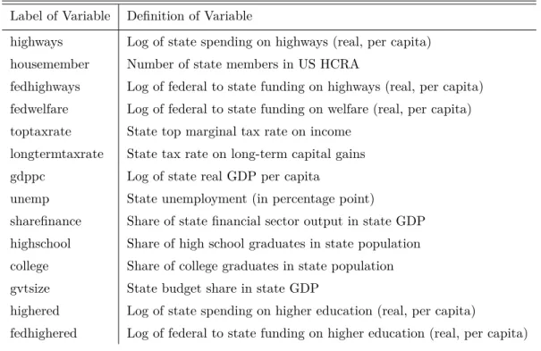
Table 1: Labels and Definitions of All Variables – US Data from 1976 to 2008 Label of Variable Definition of Variable

highways Log of state spending on highways (real, per capita) housemember Number of state members in US HCRA

fedhighways Log of federal to state funding on highways (real, per capita) fedwelfare Log of federal to state funding on welfare (real, per capita) toptaxrate State top marginal tax rate on income

longtermtaxrate State tax rate on long-term capital gains gdppc Log of state real GDP per capita

unemp State unemployment (in percentage point)

sharefinance Share of state financial sector output in state GDP highschool Share of high school graduates in state population college Share of college graduates in state population gvtsize State budget share in state GDP

highered Log of state spending on higher education (real, per capita)

fedhighered Log of federal to state funding on higher education (real, per capita)

one can interpret as redistribution having a reducing effect on inequality. However, only the former is significant. More surprisingly, the top marginal income tax rate has a positive sign but is hardly significant while the unemployment rate turns out to have a negative sign and to be highly significant. As in previous studies, the share of the financial sector in the state’s economy has a positive coefficient, the significance of which is less stable than the unemployment rate or the long-term tax rate. While the college graduation rate is not significant, the high school graduation rates is clearly significant. GDP per capita has a positive coefficient that is significant. Finally, federal funding for highways is found to increase inequality, consistent with our interpretation, though its coefficient is not significant. While the first-stage F statistic is around 6 in column (2), the corresponding p-value is reassuringly below 2% and the null hypothesis – that our endogenous variable is in fact exogenous – is rejected at a 3% significance level. Note that all our results rely on (heteroscedasticity-robust) standard errors that are clustered at the state level, to take into account possible autocorrelation within but not across states.

To alleviate the concern that increasing membership to the House of Representative Committee on Appropriations by a given state may not be a particularly strong predictive indicator of state spending on highways, we add a second set of instruments, which include spending itself, lagged from 2 to 10 years, as is common practice. Even though lagged values of the endogenous variables are less appealing as instruments than say, committee membership, particularly from an economic standpoint, they are still useful to gain precision in the estimate and to possibly detect violations of the exclusion restriction. Column (3) of Table2

shows the outcomes of the over-identified model with 10 instruments (9 lags for spending in addition to the number of committee members), which is more precisely estimated and has a first-stage F statistic around 14. In addition, the assumption that instruments and errors are uncorrelated is not rejected, as can be seen from the overidentification test p-value of 33% (based on the Hansen-J statistic). In addition, column

Table 2: Top 1% Income Share and Spending on Highways – 2SLS Estimation

Dependent Variable Top 1% Income Share

(1) (2) (3) (4)

OLS IV 1 instr. IV 10 instr. LIML 10 instr.

highways -0.158 -4.047** -0.937* -1.008* (0.216) (1.752) (0.520) (0.560) L3.fedhighways 0.064 0.134 0.078 0.079 (0.114) (0.289) (0.135) (0.137) fedwelfare -0.414 -0.799* -0.491 -0.498 (0.337) (0.443) (0.329) (0.329) toptaxrate 0.032 0.133 0.052 0.054 (0.105) (0.128) (0.103) (0.103) longtermtaxrate -0.223*** -0.177* -0.214*** -0.213*** (0.081) (0.093) (0.078) (0.078) gdppc 3.906*** 7.070*** 4.540*** 4.598*** (0.945) (2.388) (1.196) (1.226) unemp -25.296*** -22.744*** -24.784*** -24.737*** (5.679) (7.042) (5.517) (5.519) sharefinance -1.554 3.530 -0.535 -0.442 (4.943) (6.505) (5.112) (5.131) highschool -5.688* -1.226 -4.793* -4.712 (2.916) (4.258) (2.880) (2.890) college -2.461 4.103 -1.145 -1.025 (3.865) (5.861) (4.221) (4.266) gvtsize -0.885 -0.710 -0.850 -0.847 (1.096) (1.311) (1.107) (1.109) Observations 1443 1443 1443 1443 R2 _{0.927 0.881 0.925 0.925}

First-stage F -stat n.a. 6.13 13.70 13.70

F -test p-value n.a. 0.016 0.000 0.000

Overident. test p-value n.a. n.a. 0.33 0.33

Endog. test p-value n.a. 0.025 0.14 0.14

See Table1for labels of variables

All regressions include time and state fixed effects as well as state-specific time trends Standard errors clustered at state level in parentheses

* p < 0.10, ** p < 0.05, *** p < 0.01

(4) of Table2further tests for possible weak identification by reporting the outcome of using the Limited Information Method Likelihood (LIML) estimator. The resulting LIML coefficients in column (4) are close to those in column (3), and the overall prediction of our analysis is that a 1% increase in spending on highways reduces the top 1% income share by about 1 to 4 percentage points. This is arguably a nontrivial effect.

In the spirit of Chernozhukov and Hansen (2008), since a first-stage statistic F below 10 does not necessarily invalidate the IV analysis, to further check on the validity of our instruments, in Table 3 we also report through OLS the reduced-form coefficients that are obtained when we estimate our dependent variable on our instruments and covariates. Columns (1), (2) and (3) show the estimates that we obtain when the instruments are committee membership, lagged spending on highways and both, respectively. Basically, the first row in Table3reveals that an additional committee member increases the top 1% income share by about 0.2 percentage point.

To carry out additional robustness checks of results presented in Table2, we report (in Tables4-5) the estimates, we obtain using other measures of income inequality in lieu of the income shares of the top wealthiest 1% of the population, as the dependent variable in our IV regressions. We again use lags of up to 2 years and essentially obtain similar results, except for the Gini index. As for the latter, one explanation is that in the context of a truncated income distribution constructed from tax forms, the Gini coefficient may be a biased measure of inequality. As a result, the Gini index gives a more distorted picture than all the other inequality measures and bears no relationship with investment on highways. Although the results from the reduced-form specification are not reported (to save space), in which various measures of inequality are regressed directly on our instrument and all controls are reassuring, they reveal a significant coefficient for the number of committee members. In addition, it seems reasonable to assume that the number of committee members has no direct effect on inequality, but rather affects it through spending on highways, as confirmed by the first-stage results reported in the next section. In other words, the exclusion restriction is likely to be met. This is confirmed in AppendixA.4, where we report further evidence that rejects violations of the exclusion restriction. In addition, AppendixA.2extends our results by considering additional lags for both the instrument and the endogenous variable, which leads us to the conclusion that state spending affects income inequality within a couple of years. Finally, AppendixA.3shows that similar results hold when spending on higher education and lagged inequality are added as controls.

As noted in the introduction, Aghion et al. (2016) have shown that the number of members in the Senate Committee on Appropriations is a powerful instrument to identify exogenous variations in innovation. However, Aghion et al. (2016) report that more federal funding for highways increases the top 1% income share (see their Table 10 for example). This is consistent with the positive sign of the coefficient on federal funding for highways (fedhighways) in Tables2and4-5above.6 In fact, Aghion et al. (2016) aim at capturing the effect of innovation on inequality and they use federal funding for highways as a control variable. Such a strategy shows that the ascension of a congressman to membership in the Senate Committee on Appropriations triggers positive shocks in federal grants earmarked to research universities, or to highways for that matter. The latter type of grants is not fundamental in their analysis since they focus on how

6_{It is important to stress that federal funding for highways and state spending on highways do not coincide because} (i) federal funds are to a large extent fungible, and (ii) states use other resources to finance infrastructure investments, such as taxes.

Table 3: Top 1% Income Share and Spending on Highways – Reduced Form and First Stage Dependent Variable Top 1% Top 1% Top 1% highways highways highways

(1) (2) (3) (4) (5) (6)

OLS OLS OLS OLS OLS OLS

L2.housemember 0.218*** 0.205*** -0.054*** -0.036** (0.078) (0.076) (0.021) (0.015) L6.highways 0.324* 0.312* -0.046 -0.044 (0.174) (0.175) (0.035) (0.035) L3.fedhighways 0.081 0.081 0.092 0.013 -0.025 -0.027 (0.112) (0.113) (0.112) (0.060) (0.048) (0.048) fedwelfare -0.400 -0.432 -0.425 -0.099 -0.043 -0.044 (0.346) (0.331) (0.336) (0.089) (0.071) (0.070) toptaxrate 0.031 0.026 0.027 0.025 0.015 0.015 (0.102) (0.108) (0.106) (0.024) (0.021) (0.020) longtermtaxrate -0.235*** -0.217*** -0.228*** 0.014 0.008 0.010 (0.082) (0.078) (0.078) (0.017) (0.013) (0.013) gdppc 3.752*** 3.989*** 3.942*** 0.820*** 0.632** 0.640** (0.900) (0.935) (0.929) (0.316) (0.257) (0.257) unemp -25.243*** -25.996*** -25.933*** 0.618 0.080 0.069 (5.640) (6.136) (6.083) (1.343) (0.978) (0.975) sharefinance -1.751 -1.786 -1.902 1.305 0.494 0.514 (4.854) (5.177) (5.111) (0.914) (0.616) (0.624) highschool -5.770** -5.353** -5.312** 1.123* 0.657 0.649 (2.874) (2.729) (2.665) (0.602) (0.610) (0.596) college -3.804 -2.320 -3.377 1.954** 1.416** 1.599** (3.663) (3.770) (3.722) (0.807) (0.671) (0.681) gvtsize -0.945 -0.803 -0.853 0.058 0.011 0.020 (1.076) (1.095) (1.073) (0.179) (0.149) (0.146) Observations 1443 1443 1443 1443 1443 1443 R2 _{0.928 0.927 0.928 0.759 0.787 0.789}

See Table1for labels of variables

All regressions include time and state fixed effects as well as state-specific time trends Standard errors clustered at state level in parentheses

* p < 0.10, ** p < 0.05, *** p < 0.01

Table 4: Various Inequality Measures and Spending on Highways – 2SLS with 1 Instrument Dependent Variable Top 1% Top 0.1% Top 0.01% Theil Atkinson Gini

(1) (2) (3) (4) (5) (6)

IV 1 instr. IV 1 instr. IV 1 instr. IV 1 instr. IV 1 instr. IV 1 instr.

highways -4.047** -3.453** -2.538** -0.238** -0.034 0.001 (1.752) (1.612) (1.188) (0.101) (0.033) (0.048) L3.fedhighways 0.134 0.102 0.068 -0.007 -0.004 0.006 (0.289) (0.225) (0.161) (0.012) (0.003) (0.004) fedwelfare -0.799* -0.727** -0.479** -0.022 0.002 -0.003 (0.443) (0.304) (0.224) (0.026) (0.010) (0.012) toptaxrate 0.133 0.099 0.075 0.004 0.003 0.001 (0.128) (0.108) (0.080) (0.007) (0.003) (0.004) longtermtaxrate -0.177* -0.077 -0.012 -0.010* -0.007*** -0.007* (0.093) (0.071) (0.050) (0.005) (0.002) (0.004) gdppc 7.070*** 5.183*** 3.517*** 0.509*** 0.098* -0.044 (2.388) (1.867) (1.231) (0.134) (0.051) (0.069) unemp -22.744*** -17.804*** -10.394** -2.402*** -0.944*** 0.209 (7.042) (6.276) (4.504) (0.488) (0.166) (0.142) sharefinance 3.530 0.191 -1.455 -0.433 -0.099 0.412** (6.505) (4.897) (3.577) (0.489) (0.190) (0.170) highschool -1.226 -2.181 -0.153 0.143 -0.030 -0.278** (4.258) (3.621) (2.531) (0.263) (0.077) (0.110) college 4.103 5.532 4.536 0.842** 0.188 0.189 (5.861) (4.857) (3.253) (0.356) (0.155) (0.155) gvtsize -0.710 -0.776 -0.348 0.135 0.009 -0.092** (1.311) (0.994) (0.636) (0.086) (0.031) (0.045) Observations 1443 1443 1443 1443 1443 1443 R2 _{0.881 0.826 0.746 0.938 0.975 0.901} First-stage F -stat 6.13 6.13 6.13 6.13 6.13 6.13 F -test p-value 0.016 0.016 0.016 0.016 0.016 0.016

Endog. test p-value 0.023 0.054 0.049 0.027 0.55 0.99

See Table1for labels of variables

All regressions include time and state fixed effects as well as state-specific time trends 14

Table 5: Various Inequality Measures and Spending on Highways – 2SLS with 10 Instruments

Dependent Variable Top 1% Top 0.1% Top 0.01% Theil Atkinson Gini

(1) (2) (3) (4) (5) (6)

IV 10 instr. IV 10 instr. IV 10 instr. IV 10 instr. IV 10 instr. IV 10 instr.

highways -0.937* -0.824* -0.586* -0.082*** -0.030** -0.006 (0.520) (0.456) (0.317) (0.032) (0.014) (0.017) L3.fedhighways 0.078 0.054 0.033 -0.010 -0.004 0.006 (0.135) (0.097) (0.067) (0.006) (0.003) (0.004) fedwelfare -0.491 -0.467* -0.286 -0.007 0.003 -0.004 (0.329) (0.252) (0.176) (0.023) (0.010) (0.011) toptaxrate 0.052 0.031 0.025 0.000 0.003 0.001 (0.103) (0.080) (0.054) (0.007) (0.003) (0.004) longtermtaxrate -0.214*** -0.108* -0.035 -0.011** -0.007*** -0.007* (0.078) (0.060) (0.040) (0.005) (0.002) (0.004) gdppc 4.540*** 3.045*** 1.930*** 0.382*** 0.095** -0.039 (1.196) (0.841) (0.541) (0.067) (0.039) (0.048) unemp -24.784*** -19.529*** -11.675*** -2.504*** -0.947*** 0.214 (5.517) (4.827) (3.328) (0.418) (0.160) (0.135) sharefinance -0.535 -3.246 -4.006* -0.637 -0.104 0.421** (5.112) (3.315) (2.240) (0.438) (0.191) (0.164) highschool -4.793* -5.197** -2.391* -0.036 -0.035 -0.270*** (2.880) (2.205) (1.353) (0.196) (0.077) (0.088) college -1.145 1.095 1.243 0.579** 0.182 0.201 (4.221) (3.192) (1.904) (0.251) (0.135) (0.146) gvtsize -0.850 -0.894 -0.436 0.128* 0.009 -0.092** (1.107) (0.806) (0.472) (0.074) (0.031) (0.044) Observations 1443 1443 1443 1443 1443 1443 R2 _{0.925 0.897 0.863 0.958 0.976 0.901} First-stage F -stat 13.70 13.70 13.70 13.70 13.70 13.70 F -test p-value 0.000 0.000 0.000 0.000 0.000 0.000

Overident. test p-value 0.33 0.50 0.34 0.59 0.69 0.38

Endog. test p-value 0.14 0.30 0.44 0.007 0.11 0.84

See Table1for labels of variables

All regressions include time and state fixed effects as well as state-specific time trends Standard errors clustered at state level in parentheses

* p < 0.10, ** p < 0.05, *** p < 0.01

funding for research university facilities improve innovation. The positive coefficient that they obtain on highways should not be erroneously interpreted as a causal effect on inequality by increasing actual state spending on highways. Our results show that, quite to the contrary, the causal effect goes in the opposite direction once variations in state level spending on highways are properly instrumented by the number of committee members. Rising income inequality within a two-year horizon turns out to be caused by cuts in state level spending on highways due to exogenous variations in the number of committee members. This pattern is presented in the following section, where we discuss the first stage of our estimation strategy.

3.2

The Crowding-out Effect of Federal Grants on State Spending

In columns (4) to (6) in Table3, we draw attention to the outcome of the first stage in the IV regression that corresponds to the second stage in columns (2) to (4) of Table2 and to the corresponding reduced form in Columns (1) to (3) of Table3. The first row of Table3 shows that when a given state gains an appropriations committee member, it typically slashes investment on highways, and this is consistent with the earlier literature on the so-called “crowding-out effect” of federal grants on state spending. The spending cut can take also up to two years, as shown in Table3. The point estimates in the first row of Columns (4) − (6) in Table3show that getting an additional committee member implies a reduction of state spending on highways between 4 and 5 percentage points, which is not of trivial size. Given the second-stage estimate, this would translate into an increase of the top 1% income share of about 6 percentage points within a time period of two years.

The negative correlation between state spending on highways and the number of appropriations committee members for any given state turns out to be very significant. This pattern or trend coincides with earlier results obtained by Knight (2002) who used membership in Transportation Committee. More recently, Dupor (2017) has documented a similar pattern in the context of the American Recovery and Reinvestment Act (ARRA), President Obama’s stimulus plan implemented at the outset of the 2008 global economic recession.7 In addition to the political-economy interpretation that Knight (2002) ascribes to the crowding-out effect, we conjecture that balanced-budget requirements which virtually all states have introduced in their legislative process are important to understand why additional federal funds generate cuts in both spending and taxes. To flesh out such a simple idea, we now provide a reduced-form toy model that illustrates how preference for tax cuts over public spending can lead to crowding-out under balanced-budget.8 Imagine that an hypothetical state governor has Stone-Geary-type preferences given by α log(I − I∗) − β(T − T∗), where I stands for realized infrastructure investments, say, on highways, and T account for the taxes paid by the governor’s constituency. The starred variables I∗and T∗stand for some corresponding baseline levels. Such preferences arise, for instance, if the probability for the state governor to be elected goes up with state spending but down with taxes collected on state residents’ incomes. In other words, spending more and taxing less improve the perspective of the incumbent candidate and governor in power to be elected or reelected. The state governor’s budget constraint is given by I = T + F , where F is federal funding and is

7_{Leduc and Wilson (2017), however, find that crowding-out was absent in their analysis of the ARRA, presumably} because the Great Recession in 2008 forced states to implement policies aimed at stimulating the local economy, much like ARRA was designed as a federal stimulus package. In contrast, Knight (2002) analyzes the period from 1983 to 1997 during which no commensurately large recession occurred.

Figure 1: Massachusetts -2 0 2 4 1970 1980 1990 2000 2010

MA

taken for simplicity as given by a given state. The governor then chooses I that maximizes α log(I − I∗) − β(T − T∗), which delivers an optimal investment level given by Iopt= −αF/(β − α) + (βI∗− αT∗

)/(β − α). Provided that the governor has a preference over taxing less relative to spending more (that is, if β > α), spending on infrastructure Ioptgoes down when the state gets additional federal funding, that is, if F rises. The rationale for this is that optimal taxes, expressed as Topt= −βF/(β − α) + (βI∗− αT∗

)/(β − α), also go down when F increases. In summary, the trade-off between taxes and spending is resolved by reducing the former at the expense of a fall in the latter.

In order to get a clearer understanding and a visual perspective of the data, showing the negative relationship between the number of appropriations committee members and the level of investment on highways, we discuss two noteworthy cases. In Figure1, we plot both variables against time for the state of Massachusetts. Both the number of seats in the appropriations committee and the (log of) of real spending on highways are shown to be flat from 1970 to 1990. However, both variables start trending in opposite directions, starting in 1990, with the number of committee members going down and investment in highways rising in the first half of the 1990’s. Loosing committee members coincide with spending more on highways.

Given the insights we obtained from reviewing the data on Massachusetts, we carry out an event study for all US States. In doing so, we isolate all years for each state when the numbers of committee members grew or declined by one unit, which represents the vast majority of all variations in change of numbers of committee seats. For each year, we compute the average variation in spending on highways during a time window of three years before and three years after such unitary variation in the number of seats the state has in the appropriations committee. Figures 2 and 3 plot the evolution of spending when the number

of committee members goes down or up, respectively. The pattern that clearly emerges is consistent with the crowding-out effect, by which the number of committee members and spending on highways move in opposite direction. In addition, Figures2and3reveal that the crowding-out effect is not symmetrical, as the level of investments on highways declines more when there is an increase in the number of committee members than it goes up (prompted by higher state spending on infrastructure) when committee members fall in numbers. Although the standard errors appear to be large, the pattern reported in Figures2and

3confirm the first-stage regression result in Table3, which shows that the number of committee members and the (log) level of spending on highways correlate negatively and significantly.

4

Further Discussion

4.1

Inside the Black Box: the Role of the Construction Sector

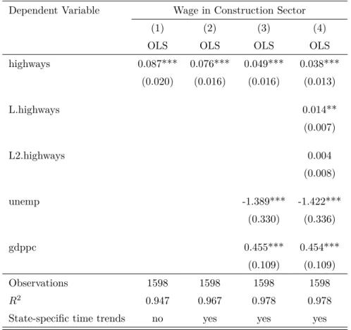
Section 3 documents that the causal chain from rising spending on highways to inequality reduction operates at time horizons shorter than two years. This fact suggests that the construction sector might be important in channeling at least part of the suggested causal effect. In line with such intuitive reasoning, we now provide suggestive evidence that rising spending on highways goes hand in hand with an increasing wage paid by the construction sector.9 Figure4reports a scatter plot of our two variables of interest, which clearly exposes how spending on highways and the wage paid in the construction correlates positively. Such eye-ball econometrics is formally confirmed by Table6, which reports regression results where the dependent variable is the construction wage. Column (1) in Table 6shows the coefficient of spending on highways when the dependent variable is the construction wage and both state and time fixed effects. Column (2) adds state-specific time trends, while column (3) further adds the unemployment rate and GDP per capita as covariates. All variables are highly significant and have the expected sign: the wage and the level of unemployment go in opposite directions while the wage and the level of economic activity go hand in hand at the state level. The point estimate indicates that a 1% increase in spending on highways is associated with an increase in the construction wage of about 5 basis points. Column (4) in Table6finally shows that spending with a one-year lag also correlates positively with the wage paid in the construction sector. This is consistent with our findings in Section3, which show that spending on highways affects income inequality within a couple of years.10

We are fully aware that the evidence reported above is only suggestive that more spending on highways at the state level reduces income inequality through a booming construction sector. To further test such a hypothesis, we would like to go beyond top shares and investigate which parts of the income distribution are most affected by investments in transportation infrastructure. We are of the view stronger impacts may be expected on lower percentiles, if it is indeed the case that more construction jobs drive some people out

9_{Our measure of the wage in the construction sector is constructed from BEA data. We divide the wages and} salaries by employment (respectively series SA7 and SA25, available in the Annual State Personal Income and Employment section athttps://www.bea.gov/regional/index.htm), both from the private non-farm construction sector.

10_{In addition, unreported results show that all the indices of income inequality we use correlate negatively with} the construction wage lagged within one or two years. This provides further evidence that a rising wage in the construction sector contributes to inequality reduction.

Figure 2: Event Study – Fall in State Spending on Highways .6 .8 1 1.2 1.4 1.6 h o u se me mb e r -. 1 5 -. 1 -. 0 5 0 .05 .1 lo g h ig h w a ys -4 -2 0 2 4 t loghighways loghighways-s.d./loghighways+s.d. housemember

Figure 3: Event Study – Rise in State Spending on Highways

.5 1 1.5 2 h o u se me mb e r -. 1 -. 0 5 0 .05 .1 lo g h ig h w a ys -4 -2 0 2 4 t loghighways loghighways-s.d./loghighways+s.d. housemember 19

of lower-pay jobs, thus reducing inequality. Unfortunately, the data on lower percentiles of the US income distribution at the state level is not yet available.11

Figure 4: Wage in Construction Sector and Spending on Highways

-2

0

2

4

6

wage in construction sector (in log)

-3 -2 -1 0 1 2

spending on highways (in log)

4.2

Policy Implications

A noteworthy feature in the empirical results discussed in Section3is that accession of a particular elected representative from, say, the state of California to the Appropriations Committee is largely exogenous to the economic situation to his or her state. The reason being is that newly available seat is withdrawn from another state, for example, such as Wisconsin, due to an existing committee member failing to be re-elected or due to loss of life. Either way, a vacancy filled by a Californian representative, largely because of partisan balance and seniority in the House, is almost a random assignment since it has nothing to do with the level of inequality in California or with any other economic outcome in California for that matter. This is why IV estimation is attractive given our data to uncover a possible causal effect from infrastructure spending to income inequality. The two-step chain in the IV estimation delivers stark results. In the first stage, as reported in Section3.2, the number of committee members in a particular state turns out to be a rather appropriate instrument for spending on highways in that particular state. This outcome coincides with the earlier empirical literature (Knight, 2002), which shows that getting an additional committee member in the transportation authorization committee triggers federal grants to finance expenditures on highways which, in turn, typically leads to a reduction of state spending on highways, the so-called “crowding-out” effect.12

As mentioned earlier, the fact that almost all states have balanced-budget constraints is probably important

11_{Private correspondence with Estelle Sommeiller in February 2018 suggests that such data will eventually become} part of the Wealth and Income Database, though.

12_{See for example Bradford and Oates (1971) for an early political-economy model of the crowding-out effect of} federal grants on state spending.

Table 6: Wage in Construction Sector and Spending on Highways Dependent Variable Wage in Construction Sector

(1) (2) (3) (4)

OLS OLS OLS OLS

highways 0.087*** 0.076*** 0.049*** 0.038*** (0.020) (0.016) (0.016) (0.013) L.highways 0.014** (0.007) L2.highways 0.004 (0.008) unemp -1.389*** -1.422*** (0.330) (0.336) gdppc 0.455*** 0.454*** (0.109) (0.109) Observations 1598 1598 1598 1598 R2 _{0.947 0.967 0.978 0.978}

State-specific time trends no yes yes yes

See Table1for labels of variables

All regressions include time and state fixed effects Standard errors clustered at state level in parentheses * p < 0.10, ** p < 0.05, *** p < 0.01

to understand why on average the addition of a new committee member leads to a cut in state spending. From the second-stage results detailed in Section 3.1, we learn that the crowding-out effect has adverse effects on income inequality: when the representative from California gets appointed on the committee, the state of California slashes spending on highways within a few years. As a consequence, jobs are lost in the construction sector and people who are fired end up in a lower position in the income distribution. At the end of such a causal chain, therefore, a reduction in the spending on highways leads to an increase in income inequality. Of course, the mechanism works both ways. For example, the case of Massachusetts illustrated in Figure1shows that the loss of committee members in the 1990s triggered a significant increase in spending on highways, which was accompanied by a reduction in the income share of the top 1%.13

13_{The Central Artery/Tunnel Project (CA/T), widely known as the “Big Dig” (to address traffic congestion)} represents the first time where the entire federal interstate construction funding formula was altered by Congress by authorization rather than appropriations law to benefit a specific project in a specific state. The “Big Dig” was budgeted at a cost of $2.55 billion USD, but eventually amounted to over $8 billion USD, due to cost overruns, corruption, mismanagement and faulty execution. It is the costliest highway project recorded in US history. The chart on Massachusetts thus should be viewed as an aberration, or an exception to the rule, especially with respect

We argue that some important policy implications can be drawn from our main empirical results. First, in the context of the US, our analysis reveals that there are adverse effects of federal funding through appropriations committees. As summarized above, the existence of a crowding-out effect means that an additional committee member translates into lower state spending on highways, which in turn causes rising inequality. This suggests that there are several problems associated with the indirect allocation of federal grants through congressional committees. Nothing prevents states to cut their spending when they get additional funding from the federal government, and both our analysis and anecdotal evidence suggest that there are large incentives to pursue such as path. In other words, unless the allocation process imposes some clauses that forbid recipient states to slash their spending when they receive federal grants, the causal chain described above is at play. Surprisingly enough, such no-spending-cut constraints have sometimes been imposed but not consistently over time or over spending items. For example, Dupor (2017) discusses this issue in the context of the American Recovery and Reinvestment Act that started in 2009, and reports that a no-spending-cut clause applied to the education segment of the stimulus plan but not to the funds allocated for investment on highways. There is no clear reason why this was the case but it stands to reason to assume that the arguments in favor of similar clauses should not differ much depending on the spending item that is financed by the federal budget. Similarly, even with cases against stringent rules – because discretion should be preferred over strict rules in the context of state spending – they should not depend on which item that limited resources should be spent on. In addition, one possible limitation of allocating federal grants through appropriation committees is that it is in effect a zero-sum game. The institutional framework appears to be flawed, because when one state wins a seat, another state loses one. This means that gaining or loosing political accession to such committees might create unnecessary randomness in state spending that have large economic effects, such as investment in transportation infrastructure. Imposing explicit no-spending-cut clauses, however, would help to mitigate this source of uncertainty.

Grants from national governments to sub-national administrative bodies are not unique features that characterize industrially advanced countries. It is very plausible that low-income developing economies also experience similar governance challenges . Substantiating such a claim is however beyond the scope of this study. Nonetheless, such a reasonable assumption suggests that our methodology could in principle be helpful to measure the extent to which investments in infrastructure have a causal impact on income inequality and on the dispersion of other key social indicators such as health and education. In view of our case study based on US data, to make sure that federal spending has desired effects, as opposed to unintended adverse outcomes at a local level, greater transparency should be imposed. One possible policy measure that would contribute towards meeting this objective at a national and global level is the development of infrastructure investment platforms.14 The idea is that web-based, open-access platforms where infrastructure needs and sources of funding are matched could provide enough transparency to ensure that local governments actually spend the money where they should. Most importantly, such investment platforms would help to monitor possible leakages and other losses due to corruption.15. The benefits of

to other listed states to identify a causal link between reduced state spending on infrastructure and an increase of membership to the HRCA.

14_{See Section 5.2 in Hooper et al. (2018) and the references therein for a more detailed discussion of investment} platforms.

15_{An illuminating discussion of the former aspect in the context of a cost-benefit analysis of electrification projects} in Africa appears in Lee et al. (2016).

enhancing transparency are obvious for the potential beneficiaries of such investments, a large fraction of whom live in countries where the level of democratic accountability is unfortunately low. To the extent that the future lies in the development of Public Private Partnerships to finance the gigantic infrastructure investment gap around the world (see Arezki et al., 2017), such platforms would also make infrastructure a more attractive asset class for global investors, especially at times of extremely low returns on safe asset, particularly following the aftermath of the 2008 financial crisis. All these aspects are possibly relevant to think about policies that would foster investments in infrastructure in many developing economies and should as such be the topics of further research and fieldwork.

5

Conclusion

To the best of our knowledge, this paper is the first of its kind which draws attention to a causal relationship between investment on highways and income inequality by employing US state-level data from 1976 to 2008. We carried out IV estimations to test for causality, not because we subscribe to the view that members from each state in the US House of Representatives Committee on Appropriations (HRCA) would have a direct impact on income inequality. Instead, our aim is to empirically examine whether the HRCA would have an indirect effect through federal funding on highways spending at a state level. Our results are consistent with earlier research work by by Aghion et al. (2009,2016), which shows that state membership in the Senate Committee on Appropriations is a better instrument than membership in other types of authorization committees. The contribution of our paper to this literature is twofold. Firstly, our results indicate that on average, accession to the HRCA by an elected member from a given state is accompanied by a reduction in state level spending on highways. Secondly, they reveal that decreasing state level spending on highways can cause income inequality to rise over a period of just a few years.

One of the main aims of the paper has been to shed light on governance challenges associated with federal transfers to states and to empirically test whether infrastructure investments can contribute to reducing inequality, and potentially to promote long-term sustainable growth. A recent World Bank study (2015) points to infrastructure investments as being the main driver behind the notable increase (approximately 50 percent) in economic growth in Sub-Saharan Africa over the past decade. The same study also attributes approximately a 6 percent rise in growth of real income in China in 2007 to infrastructure spending from 1990-2005 (amounting to US $600 billion) to upgrade roads and to build expressway networks to link all of the large cities in the country. Further examples cited in the World Bank Report about infrastructure development serving as an effective policy mechanism to generate economic growth, include the US $1 trillion earmarked by India for infrastructure development up to 2020. Indirectly, however, we maintain that reducing inequality through infrastructure investments even when the economy is on a stable path -can produce long term sustainable growth, as opposed to short term growth through government stimulus programs during economic downturns. A limitation of this paper therefore is that the impact on short term growth from infrastructure investments is largely left out of the discussion. In principle, our instrument could also be used to test whether spending on highways also affects growth in a positive manner. While it is simply beyond the scope of this paper to take on this task, a promising extension would be to tackle the question of whether spending on infrastructure fosters inclusive growth. More specifically, from a policy perspective, a pressing issue is to shed light on the extent to which the lack of investment in infrastructure