Coherent intrinsic images from photo collections
The MIT Faculty has made this article openly available.
Please share
how this access benefits you. Your story matters.
Citation
Laffont, Pierre-Yves et al. "Coherent intrinsic images from photo
collections." ACM Transactions on Graphics 31, 6 (November 2012):
202. © 2012 ACM
As Published
http://dx.doi.org/10.1145/2366145.2366221
Publisher
Association for Computing Machinery (ACM)
Version
Author's final manuscript
Citable link
https://hdl.handle.net/1721.1/129415
Terms of Use
Creative Commons Attribution-Noncommercial-Share Alike
Coherent Intrinsic Images from Photo Collections
Pierre-Yves Laffont
1Adrien Bousseau
1Sylvain Paris
2Fr´edo Durand
3George Drettakis
1 1REVES / INRIA Sophia Antipolis
2Adobe
3MIT CSAIL
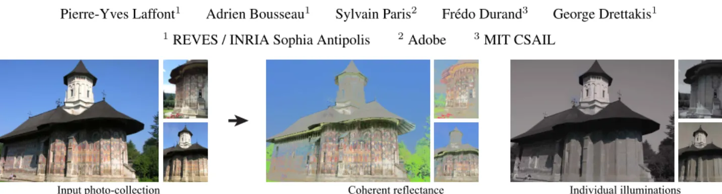
Input&photo)collection Coherent&reflectance Individual&illuminations Figure 1: Our method leverages the heterogeneity of photo collections to automatically decompose photographs of a scene into reflectance and illumination layers. The extracted reflectance layers are coherent across all views, while the illumination captures the shading and shadow variations proper to each picture. Here we show the decomposition of three photos in the collection.
Abstract
An intrinsic image is a decomposition of a photo into an illumi-nation layer and a reflectance layer, which enables powerful edit-ing such as the alteration of an object’s material independently of its illumination. However, decomposing a single photo is highly under-constrained and existing methods require user assistance or handle only simple scenes. In this paper, we compute intrinsic de-compositions using several images of the same scene under differ-ent viewpoints and lighting conditions. We use multi-view stereo to automatically reconstruct 3D points and normals from which we derive relationships between reflectance values at different lo-cations, across multiple views and consequently different lighting conditions. We use robust estimation to reliably identify reflectance ratios between pairs of points. From these, we infer constraints for our optimization and enforce a coherent solution across multi-ple views and illuminations. Our results demonstrate that this con-strained optimization yields high-quality and coherent intrinsic de-compositions of complex scenes. We illustrate how these decompo-sitions can be used for image-based illumination transfer and tran-sitions between views with consistent lighting.
Keywords: intrinsic images, photo collections
Links: DL PDF
1 Introduction
Image collections aggregate many images of a scene from a vari-ety of viewpoints and are often captured under different illumina-tions. The variation of illumination in a collection has often been seen as a nuisance that is distracting during navigation or, at best an interesting source of visual diversity. Inspired by existing work on time-lapse sequences [Weiss 2001; Matsushita et al. 2004], we
consider these variations as a rich source of information to com-pute intrinsic images, i.e., to decompose photos into the product of an illumination layer by a reflectance layer [Barrow and Tenenbaum 1978]. This decomposition is an ill-posed problem since an infin-ity of reflectance and illumination configurations can produce the same image, and so far automatic techniques are limited to simple objects [Grosse et al. 2009], while real-world scenes require user assistance [Bousseau et al. 2009], detailed geometry [Troccoli and Allen 2008; Haber et al. 2009], or varying illumination with a fixed or restricted viewpoint [Weiss 2001; Liu et al. 2008].
In this paper, we exploit the rich information provided by multi-ple viewpoints and illuminations in an image collection to process complex scenes without user assistance, nor precise and complete geometry. Furthermore, we enforce that the decomposition be co-herent, which means that the reflectance of a scene point should be the same in all images.
The observation of a point under different unknown illuminations does not help directly with the fundamental ambiguity of intrin-sic images. Any triplet R, G, B is a possible reflectance solution for which the illumination of the point in each image is its pixel value divided by R, G, B. We overcome this difficulty by process-ing pairs of points. We consider the ratio of radiance between two points, which is equal to the ratio of reflectance if the points share the same illumination. A contribution of this paper is to identify pairs of points that are likely to have similar illumination across most conditions. For this, we leverage sparse 3D information from multi-view stereo as well as a simple statistical criterion on the dis-tribution of the observed ratios. These ratios give us a set of equa-tions relating the reflectance of pairs of sparse scene points, and consequently of sparse pixels where the scene points project in the input images. To infer the reflectance and illumination for all the pixels, we build on image-guided propagation [Levin et al. 2008; Bousseau et al. 2009]. We augment it with a term to force the esti-mated reflectance of a given 3D point to be the same in all the im-ages in which it is visible. This yields a large sparse linear system, which we solve in an interleaved manner. By enforcing coherence in the reflectance layer we obtain a common “reflectance space” for all input views, while we extract the color variations proper to each image in the illumination layer.
Our automatic estimation of coherent intrinsic image decomposi-tions from photo collecdecomposi-tions relies on the following contribudecomposi-tions:
• A method to robustly identify reliable reflectance constraints between pairs of pixels, based on multi-view stereo and a sta-tistical criterion.
• An optimization approach which uses the constraints within and across images to perform an intrinsic image decomposi-tion with coherent reflectance in all views of a scene. We run our method on 9 different scenes, including a synthetic benchmark with ground truth values, which allows for a compari-son to several previous methods. We use our intrinsic images for image-based illumination transfer between photographs captured from different viewpoints. Our coherent reflectance layers enable stable transitions between views by applying a single illumination condition to all images.
2 Related Work
Single-Image Methods. Retinex [Horn 1986] distinguishes
gra-dient illumination based on magnitude, which was extended by Tap-pen et al. [2005] using machine learning. Shen et al. [2008] and Zhao et al. [2012] assume that similar texture implies the same reflectance. In contrast, Shen and Yeo [2011] assume that simi-lar chromaticity indicates same reflectance for neighboring pixels and that each image only contains a small number of reflectances. These methods work well with isolated objects [Grosse et al. 2009]. Bousseau et al. [2009] and Shen et al. [2011] require user annota-tions, whereas we need an automatic method to handle the large number of images in a collection.
Multiple-Images Methods. For timelapse sequences,
Weiss [2001] applies a median operator in the gradient do-main as a robust estimator of the reflectance derivatives. However, Matsushita et al. [2004] observe that this estimator produces poor decompositions when neighboring pixels have different normals and the input images do not cover the illumination directions uniformly. They instead use the median estimator to detect flat surfaces on which they enforce smooth illumination. Sunkavalli et al. [2007] use timelapse sequences to derive a shadow mask and images lit only by the sky or the sun. Matusik et al. [2004] additionally capture light probes to estimate a reflectance field. Our approach builds on this family of work, but we seek to handle images captured from multiple viewpoints, and avoid the sometimes cumbersome timelapse capture process.
Inverse rendering, e.g., [Yu and Malik 1998; Yu et al. 1999; De-bevec and et al. 2004] requires detailed geometric models and chal-lenging non-linear fitting. Troccoli and Allen [2008] use a laser scan and multiple lighting and viewing conditions to perform re-lighting and estimate Lambertian reflectance. In addition to a de-tailed geometry, they rely on a user-assisted shadow detector. Haber et al. [2009] estimate BRDFs and distant illumination in 3D scenes reconstructed with multi-view stereo. However, as stated by the au-thors, manual intervention remains necessary to correct the geome-try and ensure accurate visibility computation for shadow removal. In contrast, our work relies on statistical analysis and image-guided propagation to automatically estimate reflectance from incomplete 3D reconstructions, even when shadow casters are not observed in the input photographs. While our method assumes Lambertian re-flectance, it produces pixel-accurate decompositions that are well suited for image editing and image-based rendering. In contrast, to obtain pixel-accurate results, model-based approaches typically require high-precision laser-scans [Debevec and et al. 2004], rather than the less accurate multi-view stereo 3D reconstructions as used e.g., in [Haber et al. 2009]. Laffont et al. [2012] use a light probe and multiple images under a single lighting condition to reconstruct a sparse geometric representation similar to ours to constrain the intrinsic image decomposition. Their approach requires the same lighting in all views, which is not the case in photo collections. In work developed concurrently, Lee et al. [2012] use a depth
cam-era to compute intrinsic decompositions of video sequences. They constrain the decomposition in a way similar to our approach, using surface orientation and temporal coherence between frames. How-ever, they target indoor scenes with dense 3D reconstruction, while we deal with photo-collections taken under varying lighting condi-tions and with sparse 3D reconstruccondi-tions.
Photo Collections. Photo-sharing websites such as Flickrcand Picasaccontain millions of photographs of famous landmarks cap-tured under different viewpoints and illumination conditions. Photo collections of less famous places are also becoming available thanks to initiatives like the collaborative game PhotoCity [Tuite et al. 2011]. The wide availability of photos on the internet has been ex-ploited for many computer graphics applications including scene completion [Hays and Efros 2007] and virtual tourism [Snavely et al. 2006; Snavely et al. 2008]. Liu et al. [2008] extend Weiss’s al-gorithm to colorize grayscale photographs from photo collections. They use a homography or a mesh-based warping to project images on a single viewpoint. This is well adapted to images viewed from similar directions, but tends to produce blurry decompositions in the presence of large viewpoint changes.
Finally, Garg et al. [2009] apply dimensionality reduction on photo collections to estimate representative basis images that span the space of appearance of a scene. While some of the basis images model illumination effects, this “blind” decomposition does not ex-tract a single reflectance and illumination pair for each input image.
3 Overview
We take as input a collection of photographs {Ii} of a given scene
captured from different viewpoints and under varying illumination. We seek to decompose each input image into an illumination layer Siand a reflectance layer Riso that, for each pixel p and each
color channel c, Iic(p) = Sic(p)Ric(p). Furthermore, whereas
the illumination is expected to change from image to image, we assume that the scene is mostly Lambertian so that the reflectance of a point is constant across images. In the following, we drop the color channel subscript c and assume per-channel operations, unless stated explicitly.
In order to leverage the multiple illumination conditions, we need to relate scene points in different images. For this, we apply standard multiview-stereo [Furukawa and Ponce 2009] (Fig. 2(a)), which produces an oriented point cloud of the scene and estimates for each point the list of images where it appears. For ease of notation, we make 3D projection implicit and denote the value of the pixel where point p projects in image i as Ii(p).
We next infer ratios of reflectance between pairs of 3D points (Fig. 2(b)). For a pair of points (p, q), we consider the distribu-tion of ratios of pixel radiance Ii(p) / Ii(q)in all the images where
both points are visible. The ratio of reflectance is equal to the me-dian ratio of rame-diance if the two points have the same illumination in most lighting conditions. A contribution of our work is to identify pairs of points that share the same illumination based on geometric criteria and on the distribution of radiance ratios.
Our last step solves for the illumination layer at each image based on a linear least squares formulation (Fig. 2(c)). It includes the con-straints on reflectance ratios (depicted as green edges in Fig. 2(c)), an image-guided interpolation inspired by Levin et al. [2008] and Bousseau et al. [2009], and terms that force reflectance to be the same in all images (edges in magenta).
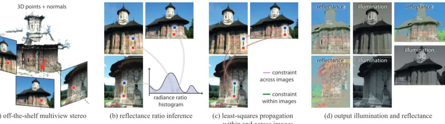
(a)$off'the'shelf$multiview$stereo (b)$reflectance$ratio$inference (c)$least'squares$propagation within$and$across$images (d)$output$illumination$and$reflectance 3D points + normals constraint across images constraint within images radiance ratio histogram reflectance reflectance illumination reflectance illumination illumination
Figure 2: Our method infers reflectance ratios between points of a scene and then expresses the computation of illumination in all images in a unified least-square optimization system.
4 Reflectance ratios
Our method relies on reflectance ratios inferred from the multiple illumination conditions. In order to relate points in different im-ages, we reconstruct a sparse set of 3D points and normals, and introduce a statistical criterion to reliably infer reflectance ratios.
4.1 Relations on reflectance between pairs of points
If two points p and q have the same normal ~n and receive the same incoming radiance, then the variations of the observed radiances I are only due to the variations of the scene reflectance R.
Assuming Lambertian surfaces, the radiance I towards the camera at each non-emissive point p is given by the following equation:
I(p) = R(p) Z
⌦
L(p, ~!) ( ~!· ~n(p)) d~! (1) where L(p, ~!) is the incoming radiance arriving at p from direc-tion ~!, ~n(p) is the normal at p, and ⌦ is the hemisphere centered at ~n(p).
Given a pair of points p and q with the same normal ~n, we can express the ratio of radiance between the two points as
I(q) I(p) = R(q) R(p) R ⌦ L(q, ~!) ( ~!· ~n) d~! R ⌦ L(p, ~!) ( ~!· ~n) d~! . (2)
If the incoming radiance L is identical for both points, then the ratio of reflectances R(q) / R(p) is equal to the ratio of radiances I(q) / I(p). From multiview stereo we have a normal estimate for each point, and it is straightforward to find points with similar normals. We next find an image where lighting conditions at p and qmatch. For points p and q which are close, the likelihood that a shadow boundary falls between them is low. Thus for most images in which these points are visible, the radiance ratio is equal to the reflectance ratio. However, lighting may still not match in a few images. Inspired by the work of Weiss [2001] and Matsushita et al. [2004] in the context of timelapse sequences, we use the median operator as a robust estimator to deal with such rare cases:
R(q) R(p) = mediani2I(p,q) ✓ Ii(q) Ii(p) ◆ (3) where the median is taken only over the images of the set I(p, q) ⇢ {Ii} in which both p and q are visible.
Ambient occlusion. Our derivation so far assumes that the illu-mination depends only on the normal orientation and is independent of the location. However, for scenes with strong concavities, differ-ences in visibility might cause two points with similar normals to have different illumination on average, because one of them might be in shadow more often. We compensate for this by evaluating the ambient occlusion factor ↵(p), that is, the proportion of the hemi-sphere visible from p. We compute ambient occlusion by casting rays from the 3D points in the upper hemisphere around the normal, and intersecting them with a geometry proxy created with standard Poisson mesh reconstruction1. The estimation of ambient
occlu-sion is robust to inaccurate geometry, since it averages the contri-bution of incoming light from all directions of the hemisphere. For points in the shadow, Eq. 2 becomes:
I(q) I(p) = R(q) R(p) ↵(q) ↵(p) (4)
We account for this by multiplying the ratio I(q)/I(p) by ↵(p)/↵(q)to correct the reflectance ratio estimated in Eq. 3.
4.2 Selection of constrained pairs
Given the set of 3D points, we need to select a tractable number of pairs whose median ratio is likely to be a good estimate of the re-flectance ratio. Based on the above discussion, we first selectively subsample the set of all possible constraints according to geomet-ric factors, i.e., normals and distance. We then discard unreliable constraints with a simple statistical criterion on the observed ratios.
Geometric criterion. For each 3D point, we select a set of can-didate pairs that follow the geometric assumptions in Sec. 4.1. In most cases, the two points of a pair should be nearby and have sim-ilar normals. However, we also wish to obtain a well-connected graph of constraints, with a few pairs consisting of points which are further apart or with varying orientations. Our approach con-sists in sampling candidate pairs by controlling the distribution of their spatial extent and orientation discrepancy. Note that this step only selects candidate pairs, on which constraints might be applied; unreliable pairs will be discarded in the next step of the algorithm. We define the distance d~non normal orientation between two points
pand q from the dot product between their normals:
d~n(p, q) =|1 ~n(p)· ~n(q)| . (5) 1In practice, we use the Poisson reconstruction in MeshLab (http://meshlab.sourceforge.net)
1 1 2 1 3 1 3 1 7 1 1 4 1 1 1 2 2 2
(a) Initial point cloud (b) Number of samples per cell (c) Final sampled points (color: d3Dto reference cell)
Figure 3: 2D Illustration of our sampling algorithm for a single point. (a) Given an oriented point cloud, we wish to select N points so that their distances d3Dand d~nto a reference point (black
square) follow normal distributions. (b) We first embed the point cloud in a grid and compute Euclidean distances to the cell con-taining the reference point; the distance is color-coded from blue to red. We infer a sampling probability for each cell based on d3Das
described in Algorithm 1, from which we draw N samples to choose the number of points to select in each cell, shown as black numbers. (c) Finally, we sample the corresponding number of points within each cell based on the normal discrepancy d~n. Note that a point
can be sampled multiple times if its cell contains too few points. We set d3D(p, q)to be the Euclidean 3D distance, representing the
spatial proximity of two points.
Our goal is to select N candidate pairs of points so that d~nand d3D
follow normal distributions N ( ~n)and N ( 3D). The parameter ~
naccounts for surfaces with low curvature and inaccuracy in the
normals estimated from multiview stereo. We set 3Dto 20% of the
spatial extent of each scene, and ~n= 0.3for all our results.
For a given point p, we sample the density functions in two steps. First we select a subset of points according to N ( 3D), and then we
sample this subset according to N ( ~n). In both cases, the major
difficulty resides in properly accounting for the non-uniform distri-bution of the distance d 2 {d~n, d3D} in the point cloud generated by
multiview stereo. We account for these non-uniform distributions with the following algorithm:
Algorithm 1 Sampling according to 3D distances or normals 1. Estimate the density of distances foriginal(d(p, q))of all points
qto the current point p. We use the Matlab ksdensity function, which computes a probability density estimate of distances to p from a set of samples d(p, q) by accumulating normal kernel functions centered on each sample.
2. Assign to each point q a sampling probability based on desired distribution N ( ) and the density of distances foriginal:
Pr(q) = exp ✓ d(p, q)2 2 2 ◆ / foriginal(d(p, q))
3. Select a subset of points according to their probabilities Pr(q) using inversion sampling.
In practice, we accelerate the sampling of N ( 3D)by first
embed-ding the point cloud in a 3D grid (with 103 non-empty cells on
average). We then apply Algorithm 1 to the grid cells instead of the points, ignoring empty cells and computing d3Dat the cell centers.
As a result of this first sampling we obtain a list of cells and the number of points that we need to choose in each cell to obtain a total of N pairs. We then apply Algorithm 1 according to d~n, with
the caveat that we only consider points from the cells that should be sampled, and we apply inversion sampling independently in each cell to select the proper number of points. We illustrate this process in Fig. 3 and supplemental materials, and provide Matlab code2.
2https://www-sop.inria.fr/reves/Basilic/2012/LBPDD12/ 0 "1.5 1.5 Log)of)radiance)ratios Probability)density (a) (b) (c) (d) point cloud
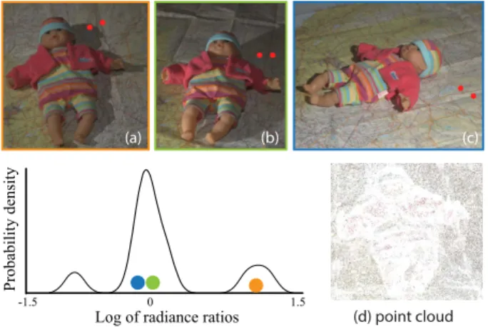
Figure 4: Analysis of the distribution of radiance ratio (red chan-nel, log scale) between two 3D points (red dots) with similar nor-mals, under varying viewpoints and lighting. The PDF has a dom-inant lobe, corresponding to (b) and (c) where both points receive approximately the same incoming radiance. In (a), the light is vis-ible from only one of the points and the corresponding radiance ratio falls in a side lobe. (d) shows the point cloud for image (a).
Our sampling strategy ensures a good distribution of pairs of points, with many “short distance” pairs around the point and a few “longer distance” pairs. We also experimented with a simple threshold that selects the pairs with the highest score based on d~nand d3D, but this
naive strategy tends to only select short distance pairs with identical normals, yielding a weakly connected graph of constraints. This results in isolated regions in the final optimization. We used 30 candidate pairs per point in all our examples, and keep at most 1.5 million candidate pairs per scene.
Cuboid scenes are seemingly problematic since pairwise constraints cannot connect orthogonal faces. However, the faces may be indi-rectly connected via other objects in the scene. The solution is also influenced by a smoothness prior (Sec. 5.2) and a coherence term (Sec. 5.3). In our experiments, these additional constraints were enough to obtain plausible decompositions even on cuboid scenes (Fig. 7, left; Fig. 9, bottom row).
Photometric statistical criterion. Each candidate pair (p, q)
can be observed in a subset of input images I(p, q). Figure 4 il-lustrates the probability density function (PDF) of the ratio of radi-ances of a pair over multiple images with varying lighting. When the two points fulfill our assumptions, the distribution has a dom-inant lobe well captured by the median operator. In such a case, the reflectance ratio of the pair can be estimated with the median. However when the two points receive different incoming radiance in more than 50% of the images, the distribution is spread and not necessarily centered at the median. We detect and reject such unre-liable pairs, by counting the observations of the radiance ratio that are far from the median value. The observation of pair (p, q) in image j is considered far from the median if
log ✓ Ij(q) Ij(p) ◆ median i2I(p,q)log ✓ Ii(q) Ii(p) ◆ > 0.15 (6) in at least one channel. We consider a pair to be unreliable if it has less than 50% of the radiance ratio values close to the median, or if it is visible in less than 5 images (too few observations). Candi-date pairs that are considered reliable will be used to constrain the intrinsic image decomposition (Sec. 5.1).
5 Multi-Image Guided Decomposition
We now have a sparse set of constraints on the ratio of reflectance at 3D points. To obtain values everywhere, we formulate an energy function over the RGB illumination S at each pixel of each image. Our energy includes data terms on the reflectance ratios, an image-guided interpolation term, and a set of constraints that enforce the coherence of the reflectance between multiple images. This results in a large sparse linear least square system, which we solve in a staggered fashion.
5.1 Pairwise reflectance constraints
Given the ratio between the reflectances of pixels corresponding to points p and q in Eq. 3, we deduce ratio Qj(p, q)between the
illumination of the corresponding pixels in image j: Qj(p, q) =Sj(p) Sj(q) = Ij(p) Ij(q) R(q) R(p) (7a) = Ij(p) Ij(q)mediani2I(p,q) ✓ Ii(q) Ii(p) ◆ (7b) where Sjis the illumination layer of image j. This equation lets us
write a constraint on the unknown illumination values: Qj(p, q)
1
2Sj(q) = Qj(p, q) 12Sj(p) (8) We combine the contribution of all the constrained pairs selected in Sec. 4.2 in all the images where they are visible, and express these constraints in a least-squares sense to get the energy Econstraints:
X j X (p,q) ⇥ Qj(p, q) 1 2Sj(q) Qj(p, q) 12Sj(p)⇤2 (9)
In practice, we have one such term for each RGB channel.
5.2 Smoothness
We build our smoothness prior on the intrinsic images algorithm of Bousseau et al. [2009] that was designed to propagate sparse user indications for separating reflectance and illumination in a single image, and on the closely related Matting Laplacian introduced by Levin et al. [2008] for scribble-based matting. The former assumes a linear relationship between the unknowns and the image channels and the latter an affine relationship. We experimented with both, and while the intrinsic image prior captures variations of illumi-nation at a long distance from the constrained pixels, we show in the supplemental materials that the matting prior yields smoother illumination in regions with varying reflectance, especially in our context where many pixels are constrained.
The matting prior translates into a local energy for each pixel neigh-borhood that relates the color at a pixel x with the illumination value in each channel Sjc(x)using an affine model:
X c2{r,g,b} X y2Wx j Sjc(y) axjc· Ij(y) bxjc 2 + ✏ (axjc)2 (10) where Wx
j is a 3 ⇥ 3 window centered on x, axj and bxj are the
unknown parameters of the affine model, constant over the window, and ✏ = 10 6is a parameter controlling the regularization (ax
j)2
that favors smooth solutions. Levin et al. [2008] showed that ax j
and bx
j can be expressed as functions of Sj and removed from the
system. Then, summing over all pixels and all images yields an
energy that only depends on the illumination, and can be expressed in matrix form: Esmoothness= X c2{r,g,b} X j ˆ STjcMjcSˆjc (11)
where the vectors ˆSj stack the unknown illumination values in
image j and the matrices Mj encode the smoothness prior over
each pixel neighborhood in this image (see the paper by Levin et al. [2008] for the complete derivation).
We found that it is beneficial to add a grayscale regularization for scenes with small concavities in shadow. Because these areas often have no (or very few) reconstructed 3D points, they are influenced by their surrounding lit areas and illumination tends to be overesti-mated. For such scenes, we add the term below to favor illumina-tion values close to the image luminance:
X x X c2{r,g,b} ⇣ Sjc(x) 1 3 ⇥ Ijr(x) + Ijg(x) + Ijb(x)⇤⌘ 2 (12) We use a small weight (10 3) so that this term affects only regions
with no other constraints. We show in supplemental material that although results are satisfying without it, this term helps further improve the decomposition.
5.3 Coherent reflectance
For photo collections, it is important to ensure that the intrinsic image decomposition is coherent across different views. We impose additional constraints across images by enforcing the reflectance of a 3D point to be constant over all views where it appears. Consider the case where a given point p is visible in two images Imand In. For each such pair (m, n) of images we want to force
the pixels corresponding to p to have the same reflectance, and thus infer a constraint on their illumination:
Rm(p) = Rn(p)) Im(p) Sm(p)= In(p) Sn(p) ) Im(p) Sn(p) = In(p) Sm(p) (13) We denote I(p) ⇢ {Ii} the subset of images where the point p is
visible. Summing the contribution of every pair of images where a point appears gives us an additional energy term Ecoherence that
encourages coherent reflectance across images: X p X m2I(p) X n2I(p) n>m Im(p) Sn(p) In(p) Sm(p) 2 (14)
This term generates a large number of constraints. We found that applying them only at the points selected in Sec. 4.2 yields equiv-alent results while reducing the complexity of the system. In addi-tion, we describe an efficient solver in Sec. 5.4.
5.4 Solving the system
We combine the energy terms defined above with weights wconstraints = 1, wsmoothness = 1and wcoherence = 10, fixed for all
our results. Minimizing this global energy translates into solving a sparse linear system where the unknowns are the illumination val-ues at each pixel of each image. We obtain the reflectance at each pixel by dividing the input images by the estimated illuminations. Our system is large because it includes unknowns for all the pixels of all the images to decompose. To make things tractable, we use an
iterative approach akin to a blockwise Gauss-Seidel solver, where each iteration solves for the illumination of one image with the val-ues in all the other images fixed. The advantage of this approach is that we can reduce Eq. 14 to a single term per point p. To show this, we first write the energy Ek
coherence(m, p)for point p in image
mat iteration k: X n2I(p) n<m Im(p) Skn(p) In(p) Skm(p) 2 + X n2I(p) n>m Im(p) S(k 1)n (p) In(p) Skm(p) 2 (15)
In this energy, the only variable is Sk
m(p), everything else is fixed.
Since all the terms in Eq. 15 are quadratic functions depending on the same variables, the energy can be rewritten as a single least-squares term, plus a constant which does not depend on Sk
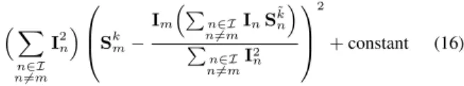
m(p): ⇣ X n2I n6=m I2n ⌘0B @Skm Im⇣Pn2I n6=mInS ˜ k n ⌘ P n2I n6=mI 2 n 1 C A 2 +constant (16)
where for clarity, we use the notation S˜k
n= Sknwhen n < m and
S(k+1)n when n > m, and omit the dependency on p.
Eq. 16 expresses the inter-images constraints on Sk
m(p)as a single
least-squares term, which shows that these constraints are tractable even though there is a quadratic number of them. Further, when we derive this term to obtain the corresponding linear equation used in our solver, the left factor and the denominator cancel out, ensur-ing that our system does not become unstable with small values of P
n2I n6=mI
2 n.
To initialize this iterative optimization, we compute an initial guess of the illumination in each image with an optimization where we only use the single-image terms Econstraints, Esmoothness, and the
grayscale regularization. The energy decreases quickly during the first few iterations of the optimization process, then converges to a plateau value. We applied 4 iterations for all the results in this paper. Intermediate results after each iteration are shown as supple-mental material.
6 Implementation and Results
3D Reconstruction. We first apply bundle adjustment [Wu et al. 2011] to estimate the parameters of the cameras and patch-based multi-view stereo [Furukawa and Ponce 2009] to generate a 3D point cloud of the scene. For each point, this algorithm also es-timates the list of photographs where it appears. We compute nor-mals over this point cloud using the PCA approach of Hoppe et al. [1992]. We used 103 images per scene on average to perform reconstruction, but this varies significantly depending on the scene (e.g., we used 11 image to reconstruct the “Doll” scene).
Point cloud resampling. Multi-view reconstruction processes
full-sized photographs, while we apply our decomposition on smaller images for efficiency. Multiple nearby 3D points may project to the same pixels on the resized images. We downsam-ple the point cloud so that at most one 3D point projects to each pixel in each image, using a greedy algorithm which gives priority to points that are visible in most images. To do so, we visit every pixel of every image, creating the point set as we proceed. At a given pixel, we first test if a point of the set already projects to it.
If not, we choose the point which is visible in the largest number of images, and we add it to the set. We finally limit the size of the point cloud to 200k points. We also discard points that project on strong edges because their radiance tends to result from a mixture of reflectances that varies among images: we discard a point if the variance of the radiance in adjacent pixels is greater than 4⇥10 3.
Performance. The average running time of our method is 90
minutes for the 9 scenes in this paper. Our unoptimized Matlab implementation of the sampling algorithm (Sec. 4.2) takes 52 min. on average and the selection of reliable constraints takes less than a minute. Each iteration of the optimization takes 6 min on average; we use Matlab’s backslash operator to solve for each image within one iteration. We could greatly speed up our method by paralleliz-ing the samplparalleliz-ing of candidate pairs for each 3D point.
6.1 Intrinsic Decompositions
We demonstrate our method on three types of data. First we apply our method to synthetic data which allows a comparison to ground truth. We then show results of our method for captured scenes in which we have placed cameras and lights around objects in a room. We finally apply our method to online photo collections.
Evaluation on a Synthetic Scene. We evaluate our method
against a ground truth decomposition that we rendered from a syn-thetic scene. We use a diffuse model of the St. Basil cathedral be-cause it contains complex geometric details and a colorful spatially varying reflectance, in addition to occluded areas that are challeng-ing for our approach (Sec. 4.1). We render the scene and compute ground truth illumination using path-tracing in PBRT [Pharr and Humphreys 2010], and obtain ground truth reflectance by dividing the rendering by the illumination. We use a physically-based sun and sky model [Preetham et al. 1999] for daylight, and captured environment maps for sunset/sunrise and night conditions. We ren-dered 30 different viewpoints over the course of three days (in sum-mer, autumn and winter). To apply our method, we sample the 3D model to generate a 3D point cloud; this allows us to evaluate the performance of our algorithm independently of the quality of multi-view reconstruction. We provide the decompositions of 6 multi-views as supplemental material, as well as all input and ground truth data. Fig. 5 provides a visual comparison of our method against ground truth, as well as state-of-the-art automatic and user-assisted meth-ods, all kindly provided by the authors of the previous work. In supplemental materials, we provide more images and comparisons to additional methods, including [Garces et al. 2012] and our imple-mentation of [Weiss 2001] extended to multiview, which is inspired by [Liu et al. 2008]. In Fig. 6 we plot the Local Mean Squared Error (LMSE, as in [Grosse et al. 2009]) of each method with respect to ground truth, averaged over all views.
For this benchmark, our approach produces results that closely match ground truth and outperform single image methods. In par-ticular, we successfully decompose the night picture while auto-matic methods fail to handle the yellow spot lights and blue shad-ows. Our method extracts most of colored texture from the illumi-nation in this challenging case. Our method also produces coherent reflectance between all views, despite the drastic change of lighting.
0 0. 5 1 1. 5 2 x 10⁵ 0.01 0.015 0.02 0.025 0.03 0.035 0.04 0.045 Number of 3D points Average LMSE
We study the robustness of our algorithm by vary-ing the number of 3D points in the point cloud, as shown in the inset graph on the right. Our approach still outperforms the best
Reflectance
Illumination
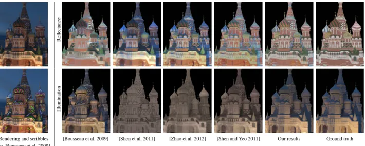
Rendering and scribbles [Bousseau et al. 2009] [Shen et al. 2011] [Zhao et al. 2012] [Shen and Yeo 2011] Our results Ground truth for [Bousseau et al. 2009]
Figure 5: Comparison to existing methods and ground truth on a synthetic rendering, generated with path tracing (see text for details). Reflectance and illumination images have been scaled to best match ground truth; sky pixels have been removed.
0 0.01 0.02 0.03 0.04 0.05 Ours [Shen1and1Yeo12011] [Zhao1et1al.12012] [Bousseau1et1al.12009] [Shen1et1al.12011] Average'LMSE
Figure 6: Numerical evaluation of five intrinsic decomposition methods. Gray bars indicate Local Mean Squared Error averaged over the three comparison images, while red bars illustrate the stan-dard deviation of LMSE across images.
single-image based
tech-nique when only 15000 points are used. We also reconstruct a point cloud with PMVS, after specifying ground truth camera pa-rameters since structure from motion techniques fail on our syn-thetic images. Our decomposition using this reconstruction yields an average LMSE of 0.01564, still significantly lower than all the approaches compared. Please see supplemental materials for the corresponding images.
Captured Scenes. We set up two indoors scenes containing
small objects and used two light sources: a camera-mounted flash with low intensity, which simulates ambient light in shadows, while a remote-controlled flash produces strong lighting from a separate direction. This setup allows us to validate our algorithm on real photographs, while avoiding the difficulty inherent in internet photo collections, such as the use of different camera settings or contrast and color manipulation that affect the validity of our assumptions. Fig. 7 shows our decomposition for the “Doll” and “Temple” scenes. We used 11 and 10 viewpoints respectively, and 7 differ-ent lighting conditions. Both scenes contain colored reflectances (cloth of the baby doll, texture of the tabletop) and strong hard shadows that are successfully decomposed by our method. Non-lambertian components of the reflectance (such as the specularities on the tablecloth) are assigned to the illumination layer, since co-herency constraints enforce similar reflectance across images. We provide as supplemental material a visual comparison between our method and previous work on a similar “Doll” scene.
Input images
Reflectance
Illumination
Figure 7: Results of our decomposition on scenes captured with a flash. Note that the colored residual in the doll illumination is due mainly to indirect light.
Internet Photo Collections. The last set of results we show is on internet photo collections of famous landmarks; we chose chal-lenging scenes with interesting lighting and shadowing effects. We download images from Flickrcor Photosynthc, avoiding pictures that have been overly edited. We use 45 images on average to com-pute the pairwise reflectance ratios (Eq. 3), and perform the intrin-sic decomposition on around 10 images per dataset. Table 1 lists the number of images used for each scene.
Input image
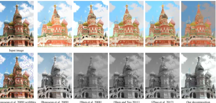
[Bousseau et al. 2009] scribbles [Bousseau et al. 2009] [Shen et al. 2008] [Shen and Yeo 2011] [Zhao et al. 2012] Our decomposition Figure 8: Comparison between our approach and existing single-image methods on a picture from an online collection. We correct radial distortion using camera parameters estimated
from scene reconstruction. We assume a gamma correction of 2.2 which is common for jpeg images. However, noise and non-linearities in the camera response can generate unreliable pixels which have very low values in some channels; in such cases we recover reliable information from other channels when available. Fig. 9 illustrates our results on several scenes, namely St. Basil, Knossos and RizziHaus. Our method successfully decomposes the input image sets into intrinsic images, despite the complex spatially-varying reflectance. In Fig. 8 we present a side-by-side comparison with four existing single-image methods on a real pic-ture of the St. Basil cathedral. We provide coherent reflectance (compare our result to Fig. 9, top row), which was not in the scope of single-image approaches. Our reflectance result is comparable in quality to the best previous work. Coherent reflectance results in some residual color in shading, although these residual are at-tenuated in other views (see Fig. 9, top row); this is discussed in Sec. 6.2.
In Fig. 1, our algorithm successfully disambiguates the complex texture on the lower facade where sparse 3D information is avail-able. However, our decomposition assigns a similar grey re-flectance to the steeple and roof of the monastery because very few 3D points are reconstructed in these areas. Without 3D points, the decomposition lacks pairwise and coherence constraints and relies mostly on the smoothness prior. Many single-image methods as-sume that pixels with similar chrominance share similar reflectance, which is likely to produce the same greyish reflectance as ours on this image, as shown in the supplemental materials.
6.2 Analysis and Limitations
Analysis. We show the number of constraints estimated for each scene in Table 1. The size of the downsampled point cloud Pseland
the number of candidate pairs for reflectance constraints Ccandare
approximately the same for all captured and downloaded scenes. However, on average 52% of the pairs are discarded for captured scenes, and 83% for downloaded scenes. Moving from a single-camera, controlled capture setting to online photo collections in-troduces errors due to different cameras, temporal extent (e.g.,
re-Input images Reflectance Illumination Figure 9: Results of our method on internet photocollections. Top: another view of the StBasil scene. The reflectance we extract is coherent with the one shown in Fig. 8. Bottom: the specular objects which cast shadows on the fac¸ade are a challenging case for multi-view stereo. Our method is able to extract their shadows despite the lack of a complete and accurate 3D reconstruction.
painted fac¸ades), and image editing. Our robust statistical criterion detects some of these errors and discards the corresponding pairs. Fig. 10 shows the effect of correcting pairwise reflectance con-straints with the ratios of ambient occlusion (Sec. 4.1). This
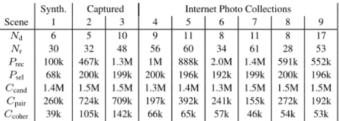
cor-Synth. Captured Internet Photo Collections Scene 1 2 3 4 5 6 7 8 9 Nd 6 5 10 9 11 8 11 8 17 Nr 30 32 48 56 60 34 61 28 53 Prec 100k 467k 1.3M 1M 888k 2.0M 1.4M 591k 552k Psel 68k 200k 199k 200k 196k 192k 199k 200k 196k Ccand 1.4M 1.5M 1.5M 1.3M 1.4M 1.3M 1.5M 1.5M 1.5M Cpair 260k 724k 709k 197k 392k 241k 155k 272k 192k Ccoher 39k 105k 142k 66k 65k 57k 46k 54k 53k
Table 1: NdNumber of images to decompose for each scene, Nr
number of images for reflectance ratio estimation (Eq. 3), Prec
num-ber of reconstructed 3D points, Pselnumber of points after
down-sampling, Ccand number of candidate pairs for reflectance
con-straints before applying statistical criterion, Cpairnumber of
reli-able pairwise constraints, Ccohernumber of coherency constraints.
1: Synthetic St. Basil; 2: Doll; 3: Temple; 4: St. Basil; 5: Knossos; 6: Moldovit¸a; 7: Florence; 8: RizziHaus; 9: Manarola.
(a) Input rendering (b) Reflectance (c) Reflectance (d) Ground truth without correction with correction reflectance Figure 10: Effect of compensating for ambient occlusion on the de-composition of a synthetic image (a). Without special treatment, the reflectance under the arches appears darker (b) because these re-gions systematically receive less illumination. Correcting the pair-wise reflectance constraints by compensating for ambient occlusion (Sec. 4.1) yields a reflectance (c) closer to ground truth (d).
rection yields a better estimation of reflectance in regions which are systematically in shadow, such as the arches in the synthetic ex-ample. Fig. 11 shows the importance of our pairwise constraints for disambiguating reflectance and illumination. In regions with complex texture, they allow us to recover smooth illumination (Fig. 11b), while relying on coherency constraints only results in strong texture artifacts in the illumination (Fig. 11a). In Fig. 12, we first show the decomposition for a single image without the coher-ence term Ecoherence, and then the result with coherence constraints
to all other images. This image contains challenging mixed light-ing conditions, i.e., the blue sky is dominant in the shadow while the bright sun is dominant elsewhere. As a result, the reflectance without coherence constraints contains a residual shadow, which is removed when coherence constraints are added. Additional exam-ples and comparisons can be found in the supplemental materials.
Limitations. We designed our method to estimate coherent
re-flectance over multiple views of a scene. However, images in photo collections are often captured with different cameras and can be post-processed with different gamma and saturation settings. Since we enforce coherent reflectance, residues of these variations are sometimes visible in our illumination component (e.g., Fig. 8). We argue that some reflectance residues in the illumination are accept-able as long as reflectance is plausible and coherent. For example they will be recombined with a coherent (thus similar) reflectance layer when transferring lighting (Sec. 6.3). Correcting for camera responses and image transformations automatically is a promising direction for future work. We expect such corrections to remove the remaining artifacts in our intrinsic image decompositions.
(a) Illumination without (b) Illumination with pairwise constraints pairwise constraints Figure 11: Influence of the pairwise relative constraints on another image of the “Doll scene”. (a) Without pairwise reflectance con-straints, texture cannot be successfully separated from lighting and the resulting illumination layer contains large texture variations. (b) Enabling these constraints allows recovering a smooth illumi-nation on the tablecloth, despite the complexity of its texture.
Input image Reflectance Reflectance without coherence with coherence Figure 12: Comparison between the decomposition, before and after multi-view coherence in the Florence scene. The coherence constraints between multiple views allow our method to recover a coherent reflectance even under mixed lighting conditions such as this bright sunset with dark blue shadows.
We rely on multi-view stereo for correspondences between views. Consequently in poorly reconstructed regions (such as very dark regions, e.g., just below the roof in Fig. 1), we rely only on the smoothness energy for our decomposition. Since no correspon-dences exist between views, reflectance in these regions is not co-herent across images. If such regions are systematically darker in all views, this is fine for lighting transfer because low illumina-tion values mask the reflectance discrepancy. However, since re-flectance is computed by dividing the input image with shading very small shading values can result as very bright pixels in the reflectance. Thin features are also problematic since radiance is blended in the input images. This could be treated with a change of scale, i.e., using close up photos.
6.3 Application to lighting transfer
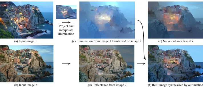
As an application of our coherent decomposition, we transfer il-lumination between two pictures of a scene taken from different viewpoints under different illumination (Fig. 13). We use the 3D point cloud as a set of sparse correspondences for which the illu-mination is known in the two images. We then propagate the il-lumination of one image to the other image using the smoothness prior of Sec. 5.2. In areas visible only in the target view, the prop-agation interpolates the illumination values from the surrounding points visible in both images. We generate a radiance image by multiplying the reflectance with the transferred illumination. Since multi-view stereo does not produce 3D points in sky regions, we use the sky detector of Hoiem et al. [2005], correct the segmentation if necessary, and apply standard histogram transfer on sky pixels.
(a)$Input$image$1 (b)$Input$image$2 Project$and interpolate illumination (c)$Illumination$from$image$1$transferred$on$image$2 (e)$Naive$radiance$transfer (d)$Reflectance$from$image$2 (f)$Relit$image$synthesized$by$our$method Figure 13: Given two views of the same scene under different lighting (a,b), we transfer the illumination from one view into the other view (c). We then multiply the transferred illumination by the reflectance layer (d) to synthesize the relit image (f). Transferring the radiance directly fails to preserve the fine details of the reflectance (e).
In Fig. 13(e) we compare our illumination transfer with direct trans-fer of radiance. Propagating the radiance produces smooth color variations in-between the correspondences. In contrast, our com-bination of transferred illumination with the target reflectance pre-serves fine details. In Fig. 14 we apply our approach to harmo-nize lighting for multiple viewpoints. In our accompanying video3
we show image-based view transitions [Roberts 2009] with har-monized photographs. Our method produces stable transitions be-tween views, despite strong shadows in the original images that could not be handled by simple color compensation [Snavely et al. 2008]. We also show artificial timelapse sequences synthesized by transferring all illumination conditions on a single viewpoint.
7 Conclusion
We introduced a method to compute coherent intrinsic image de-compositions from photo collections. Such collections contain mul-tiple lighting conditions and can be used to automatically calibrate camera viewpoints and reconstruct 3D point clouds. We leverage this additional information to automatically compute coherent in-trinsic decompositions over the different views in a collection. We demonstrated how sparse 3D information allows automatic corre-spondences to be established, and how multiple lighting conditions are effectively used to compute the decomposition. We introduced a complex synthetic benchmark with ground truth, and compared our method to several previous approaches. Our approach outperforms previous methods numerically on the synthetic benchmark and is comparable visually in most cases. In addition, our method ensures that the reflectance layers are coherent among the images. We pre-sented results on a total of 9 scenes and have automatically com-puted intrinsic image decompositions for a total of 85 images. Our automatic solution shows that the use of coherence constraints can improve the extracted reflectance significantly, and that we can pro-duce coherent reflectance even for images with extremely different lighting conditions, such as night and day. Our coherent intrinsic images enable illumination transfer and stable transitions between views with consistent illumination. This transfer has the potential to benefit to free-viewpoint image-based rendering algorithms that
3https://www-sop.inria.fr/reves/Basilic/2012/LBPDD12/
(a)$Input$images (b)$Relit$images Figure 14: We use our lighting transfer to harmonize the illumina-tion over multiple images.
assume coherent lighting when generating novel views from multi-ple photographs of a scene (e.g., [Chaurasia et al. 2011]).
Acknowledgments
This work was partially funded by the EU IP Project VERVE (www.verveconsortium.eu). INRIA acknowledges a generous re-search donation from Adobe. Fredo Durand acknowledges fund-ing from NSF and Foxconn and a gift from Cognex. We thank
Don Chesnut (Fig. 9), Dawn Kelly (Fig. 12) and the following Flickr users for permission to use their pictures: Fulvia Giannessi and Nancy Stieber (Figs. 1 and 2), L´eon Setiani (Fig. 9), SNDahl (Fig. 9), Bryan Chang (Figs. 13 and 14). We thank the authors of other methods for kindly providing comparison images included here. Thanks also to Emmanuelle Chapoulie for modeling support on the synthetic dataset, and Eunsun Lee for help with the capture of indoor scenes.
References
BARROW, H.,ANDTENENBAUM, J. 1978. Recovering intrinsic
scene characteristics from images. Computer Vision Systems.
BOUSSEAU, A., PARIS, S.,ANDDURAND, F. 2009. User-assisted
intrinsic images. ACM Trans. Graph. 28, 5.
CHAURASIA, G., SORKINE, O., ANDDRETTAKIS, G. 2011.
Silhouette-aware warping for image-based rendering. Computer Graphics Forum (Proceedings of the Eurographics Symposium on Rendering) 30, 4.
DEBEVEC, P.,AND ET AL. 2004. Estimating surface reflectance
properties of a complex scene under captured natural illumina-tion. Tech. rep., USC Institute for Creative Technologies.
FURUKAWA, Y.,ANDPONCE, J. 2009. Accurate, dense, and
ro-bust multi-view stereopsis. IEEE Trans. PAMI 32, 8, 1362–1376.
GARCES, E., MUNOZ, A., LOPEZ-MORENO, J., ANDGUTIER
-REZ, D. 2012. Intrinsic images by clustering. Computer Graph-ics Forum. EurographGraph-ics Symposium on rendering, EGSR ’12. GARG, R., DU, H., SEITZ, S. M.,ANDSNAVELY, N. 2009. The
dimensionality of scene appearance. In IEEE ICCV, 1917–1924.
GROSSE, R., JOHNSON, M. K., ADELSON, E. H.,ANDFREE
-MAN, W. T. 2009. Ground-truth dataset and baseline evaluations for intrinsic image algorithms. In IEEE ICCV.
HABER, T., FUCHS, C., BEKAERT, P., SEIDEL, H.-P., GOESELE,
M., ANDLENSCH, H. 2009. Relighting objects from image
collections. In Proc. IEEE CVPR, 627–634.
HAYS, J., ANDEFROS, A. A. 2007. Scene completion using millions of photographs. ACM TOG (Proc. SIGGRAPH) 26, 3. HOIEM, D., EFROS, A. A.,ANDHEBERT, M. 2005. Automatic
photo pop-up. ACM TOG (Proc. SIGGRAPH) 24, 3, 577–584. HOPPE, H., DEROSE, T., DUCHAMP, T., MCDONALD, J.,AND
STUETZLE, W. 1992. Surface reconstruction from unorganized
points. SIGGRAPH 26, 71–78.
HORN, B. K. 1986. Robot Vision, 1st ed. McGraw-Hill Higher Education.
LAFFONT, P.-Y., BOUSSEAU, A., AND DRETTAKIS, G. 2012.
Rich intrinsic image decomposition of outdoor scenes from mul-tiple views. IEEE Trans. on Vis. and Comp. Graph..
LEE, K. J., ZHAO, Q., TONG, X., GONG, M., IZADI, S., UKLEE, S., TAN, P.,ANDLIN, S. 2012. Estimation of intrinsic
image sequences from image+depth video. In Proc. ECCV. LEVIN, A., LISCHINSKI, D., ANDWEISS, Y. 2008. A
closed-form solution to natural image matting. IEEE Trans. PAMI. LIU, X., WAN, L., QU, Y., WONG, T.-T., LIN, S., LEUNG,
C.-S.,ANDHENG, P.-A. 2008. Intrinsic colorization. ACM,
SIG-GRAPH Asia ’08, 152:1–152:9.
MATSUSHITA, Y., LIN, S., KANG, S.,ANDSHUM, H.-Y. 2004.
Estimating intrinsic images from image sequences with biased illumination. In Proc. ECCV, vol. 3022, 274–286.
MATUSIK, W., LOPER, M., AND PFISTER, H. 2004.
Progressively-refined reflectance functions from natural illumi-nation. In Proc. EGSR, 299–308.
PHARR, M.,ANDHUMPHREYS, G. 2010. Physically Based Ren-dering: From Theory to Implementation, second edition. Morgan Kaufmann Publishers Inc.
PREETHAM, A. J., SHIRLEY, P.,ANDSMITS, B. 1999. A practical
analytic model for daylight. In SIGGRAPH, 91–100.
ROBERTS, D. A., 2009. Pixelstruct, an opensource tool for
visual-izing 3d scenes reconstructed from photographs.
SHEN, L., ANDYEO, C. 2011. Intrinsic image decomposition
using a local and global sparse representation of reflectance. In Proc. IEEE CVPR.
SHEN, L., TAN, P.,ANDLIN, S. 2008. Intrinsic image decompo-sition with non-local texture cues. In Proc. IEEE CVPR. SHEN, J., YANG, X., JIA, Y.,ANDLI, X. 2011. Intrinsic images
using optimization. In Proc. IEEE CVPR.
SNAVELY, N., SEITZ, S. M., ANDSZELISKI, R. 2006. Photo
tourism: Exploring photo collections in 3d. ACM TOG (Proc. SIGGRAPH) 25, 3, 835–846.
SNAVELY, N., GARG, R., SEITZ, S. M.,ANDSZELISKI, R. 2008.
Finding paths through the world’s photos. ACM TOG (Proc. SIG-GRAPH) 27, 3, 11–21.
SUNKAVALLI, K., MATUSIK, W., PFISTER, H., AND
RUSINKIEWICZ, S. 2007. Factored time-lapse video.
ACM Transactions on Graphics (Proc. SIGGRAPH) 26, 3.
TAPPEN, M. F., FREEMAN, W. T.,ANDADELSON, E. H. 2005.
Recovering intrinsic images from a single image. IEEE Trans. PAMI 27, 9.
TROCCOLI, A.,ANDALLEN, P. 2008. Building illumination
co-herent 3d models of large-scale outdoor scenes. Int. J. Comput. Vision 78, 2-3, 261–280.
TUITE, K., SNAVELY, N., HSIAO, D.-Y., TABING, N., AND
POPOVIC, Z. 2011. Photocity: training experts at
large-scale image acquisition through a competitive game. In Proc. SIGCHI’11, 1383–1392.
WEISS, Y. 2001. Deriving intrinsic images from image sequences.
In IEEE ICCV, vol. 2, 68.
WU, C., AGARWAL, S., CURLESS, B.,AND SEITZ, S. 2011.
Multicore bundle adjustment. In Proc. IEEE CVPR, 3057 –3064. YU, Y.,ANDMALIK, J. 1998. Recovering photometric properties
of architectural scenes from photographs. In SIGGRAPH’98. YU, Y., DEBEVEC, P., MALIK, J.,ANDHAWKINS, T. 1999.
In-verse global illumination: recovering reflectance models of real scenes from photographs. In SIGGRAPH ’99, 215–224. ZHAO, Q., TAN, P., DAI, Q., SHEN, L., WU, E.,ANDLIN, S.
2012. A closed-form solution to retinex with nonlocal texture constraints. IEEE Trans. PAMI 34.