Abstract-- Most manufacturing processes produce parts that can only be correctly measured after the process cycle has been completed. Even if in-process measurement and control is possible, it is often too expensive or complex to practically implement. In this paper, a simple control scheme based on output measurement and input change after each processing cycle is proposed. It is shown to reduce the process dynamics to a simple gain with a delay, and reduce the control problem to a SISO discrete time problem. The goal of the controller is to both reduce mean output errors and reduce their variance. In so doing the process capability (e.g. Cpk) can be increased without additional investment in control hardware or in-process sensors. This control system is analyzed for two types of disturbance processes: independent (uncorrelated) and de-pendent (correlated). For the former the closed-loop control increased the output variance, whereas for the latter it can decrease it significantly. In both cases, proper controller de-sign can reduce the mean error to zero without introducing poor transient performance. These finding were demon-strated by implementing Cycle to Cycle (CtC) control on a simple bending process (uncorrelated disturbance) and on an injection molding process (correlated disturbance). The re-sults followed closely those predicted by the analysis.
Index Terms-- Manufacturing Process Control, SPC, Dis-crete System Control, Variance Reduction
I. INTRODUCTION
ANUFACTURING processes can be controlled in a number of different ways, ranging from highly so-phisticated, high bandwidth machine and process control systems, to rather passive process monitoring. What distin-guishes "process control" from automation or machine con-trol is the inclusion of the actual material modification step in the control loop. Also of critical importance is the fre-quency of control. To achieve high frefre-quency control in-cluding the process usually involves difficult sensing and process modeling (see Hardt [1]). As a result the vast ma-jority of process control in the discrete parts industry falls into two distinct categories
* Department of Mechanical Engineering, Massachusetts Institute of Technology, Cambridge MA
** Formerly Department of Mechanical Engineering, now with Ap-plied Materials Corporation, Santa Clara, CA.
• High bandwidth control of machine state variables such as displacement, force, pressure or temperature. (ma-chine state control)
• Output sampling with process diagnostics based on measured process statistics. Statistical Process Control (SPC)
Examples of intermediate levels of control such as material state control (e.g. direct feedback of material stress, strain or temperature) are very unusual. Even less common are examples of direct process output feedback, such as in-process part geometry feedback.
A simple block diagram of a process (see Fig. 1) em-phasizes these distinctions. It also shows clearly that any control other than output feedback neglects the influence of ubiquitous process disturbances. The most common of these is the high likelihood of material property variations.
Figure 1 Three Levels of Feedback Process Control
The obvious reason for this dilemma is the cost and difficulty of making in-process measurements on a material. Even in the presence of such measurements, the resulting control system design requires a model of a process that is highly non-linear, and changing rapidly as new workpieces are introduced.
As a result we see a large gap between the high band-width, highly response methods that do not actually control the process output, and the very low bandwidth methods of statistical process control (SPC).
This paper addresses this problem by conceding that output measurements can only be made after the process cycle is complete. While this immediately limits the band-width and variance reduction performance of the system, it makes it a nearly universally applicable approach. This performance - applicability tradeoff is examined for two cases: a process contaminated with normally distributed identically distributed independent noise (or uncorrelated noise) and a similar noise process with some degree of cor-relation. It is examined both analytically and with
experi-Cycle to experi-Cycle
Manufacturing Process Control
David E. Hardt* and Tsz-Sin-Siu*
EQUIPMENT MATERIAL
CONTR.
Equipment loop
Material loop
Process output loop
ments. The latter involved processes with uncorrelated and with correlated noise.
II. BACKGROUND
One of the earliest attempts to provide a formal intro-duction to discrete feedback control in manufacturing was by Box and Kramer [2]. They argued that statistical proc-ess control and automatic procproc-ess control are similar in na-ture but originate from different industries. SPC is devel-oped for the “parts” industry, while APC is designed for the “process” industry. The two industries have different goals. The parts industry wants to achieve the smallest possible variation while the process industry wants the highest yield. Different disturbances are associated with the two indus-tries. The parts industry has small variations in material properties while the process industry has higher sensitivity to external disturbances such as temperature and pressure. Also, the cost of adjustment is high for the parts industry relative to the process industry. The authors then point out that the dividing line between the two industries is fading.
Based on some of the arguments and theories developed by Box and Kramer, Sachs et al. [3] presented one of the first applications of discrete feedback control to manufac-turing process. A real-time run-by-run (RbR) controller is implemented for a silicon epitaxy process to reduce vari-ability. Three modes of operations are used to accommo-date the common types of disturbances:
• Optimization mode using sequential design of experi-ments to locally optimize the process
• Rapid mode to quickly adjust the input to correct for large step disturbances (>2µ)
• Gradual mode to slowly adjust for slow drift distur-bances (1µ /100 runs)
An EWMA filter is used to estimate the intercept of the linear model of the process Experiments are performed on an Epitaxy Reactor and they show a 2.7 times improvement in the process capability, Cpk, in the gradual mode. The
re-sults also show the ability to reject step disturbances quickly in the rapid mode.
The authors also discuss the effect on the output if a more realistic probabilistic model is used:
Yt= α + β ⋅xt+ κ ⋅σ ⋅t+et
where κ ⋅σ ⋅t represents a drift (ramp) disturbance, κ
determines the slope of the ramp disturbance and
e
t is a white noise sequence with mean of zero and standard de-viation of σ. The result of statistical analysis shows that the asymptotic mean squared deviation (MSD), which is the expected value of the squared of the difference between the ouput Y× and the target T, has the following expression:MSD σ2 = 2b /β 2b /β −w+ κb /β w 2 (1)
The ratio is always greater than zero, which indicates that the MSD is greater than σ. One limiting case of the
equation is when κ=0 and b=β. Equation (1) becomes 2/(2-w), which is minimized at w=0. As a result, if the process has no ramp disturbance component, it is best to simply leave the process alone in open loop (with system gain, w/b, equal to zero).
Vander Wiel and Tucker [4] apply the concept of CTC feedback control to a manufacturing process. It is based on experiments of controlling intrinsic viscosity from a par-ticular General Electric polymerization process. It reiterates many of the equations and concepts proposed by Box and Kramer [2]. The main contribution of this paper to the field is the four-step application guideline that the authors pro-posed:
• Develop a time series transfer-function model of the process, including process dynamics caused by meas-urement delays.
• Design a suitable controller based on the model of the process.
• Put in SPC charts to monitor the closed-loop process to detect any unexpected events happening.
• If an SPC alarm signals, search for assignable causes and remove it if possible.
Smith and Boning [5] present an extension to the Expo-nentially Weighted Moving Average (EWMA) controller to dynamically update the EWMA weights via an Artificial Neural Network to provide better control. The effects of EWMA weights on the responses of systems with different disturbances are discussed, and the determination of opti-mal EWMA weights using disturbance state mapping is also presented.
The authors believe that the performance of a regular EWMA controller is highly dependent on the choice of the EWMA weights, and the ability to dynamically update the EWMA weight value is important for systems in which the process model does not accurately represent the true proc-ess dynamics. Simulation results show an improvement ranging from 9% in small drift and high noise processes to 38.7% in high drift and low noise processes.
Del Castillo and Hurwitz [6] discuss the concepts be-hind RbR control with particular emphasis on EWMA based controllers. The authors point out that this type of controller is well suited for processes where the cost of an output being off-target is high and where the cost of control action is relatively inexpensive. They also believe that the run-by-run control techniques are well suited for short-run discrete part manufacturing processes.
Limitations of these controllers include lagged response and sluggish performance. A self-tuning (ST) controller is presented to rectify some of these problems by separating the estimation problem from the control problem. The type of controller discussed is called “indirect ST” controller where the control equation is derived and then parameter estimates are substituted for the true values. Simulation results are presented and they shows that the ST controller could provide more robust control against a wider variety of distributions and system configurations than could certain EWMA controllers found in the literature.
Del Castillo [7] presents a self-tuning multiple-input multiple-output controller for run-by-run control. A sensi-tivity analysis is presented to show the performance of the controller under various simulated system noise combina-tions.
Valjavec and Hardt [8] is one of few research works re-lated to CtC feedback control that are not in the process industry. It provides validation that CtC control can be ap-plied effectively to discrete parts manufacturing processes. The authors develops a self-tuning feedback shape control algorithm for stretch forming on a reconfigurable forming tool. Based on empirical estimation results of process pa-rameters from calibration trials, a system identification strategy called the deformation transfer function is used to recursively estimate the tool shape required to achieve de-sired part shape. Stability is achieved for the control strat-egy on laboratory and full-scale experiments.
In addition, the same control methodology is used to compensate for the combined shape distortions in a series of manufacturing operations (stretch forming, chemical milling and trimming).
III. PROCESS MODEL FOR CYCLE TO CYCLE CONTROL
The consequence of sampling the output only after completion of the process leads to a very simple process model. If we assume that a typical discrete part manufac-turing process starts with a new workpiece and then applies directed energy on the workpiece during the cycle to Tc,
then by definition the process transients are over by the end of the cycle and no more change in the workpiece occurs. This allows the process to be modeled as a simple gain re-lating one or more inputs to the measured output. However, since we apply this control input at the start of the cycle and must wait the full cycle to measure the product, there is also a delay of at least one Tc. Any further delays will be
attrib-uted to measurement or the controller itself. Thus the process model becomes:
y
k=
K
pu
k−1 (2)where yk is the current process output and uk-1 is the control
input at the prior cycle. Thus the process has no apparent dynamics (other than the delay) when viewed after each cycle.
The essential control problem then arises from the fact that this process gain in fact is stochastic, owing primarily to material variation from workpiece to workpiece. It can also depend upon random variations in processing machine operation. Deterministic changes can also occur as material or machine changeovers occur.
Accordingly, this model must be augmented to include this random component. However, owing to the difficulty of analyzing closed-loop systems with variable gains, espe-cially if they are stochastic, we instead model this effect as additive noise. Thus the process model becomes:
yk=Kpuk−1+dk (3)
where d is a noise sequence that is either correlated or un-correlated in time.
If we transform this system using the Z-transform, Eqn 4 becomes
Y (z)=Kpz
−1
U (z)+D(z) (4)
IV. MEASURES OF PERFORMANCE
Before proceeding to controller design, it is important to set the expectations of this system. For manufacturing processes controlled at this level of granularity, there are some well-established measures of performance based on a statistical model of the process. The most common is the process capability, which measures the variation of the process relative to the design specifications. In particular the metric Cpk=min T+− µ 3σ , µ −T− 3σ
measures the deviation of the mean value (µ) of the process from the upper or lower tolerance limits T+ and T-, normal-ized by the variance of the process (3σ). (See Devor et al [9], e.g.) Thus we can measure the performance of our CtC control system on the basis of the distance of the mean or steady-state output from the target value (T) and the process variance σ.
It is also possible to use Taguchi's Quality Loss Func-tion (Devor et. al. [9]) to derive an expected cost of poor performance: E[ L]=Var[ x]+
{
E[ x]−T}
2 = σx 2+ (µ −T )2where L is the quality loss (usually expressed in cost fig-ures). Here again it is clear that the objective is to mini-mize variance and mean distance from the target. In Siu[10] this cost function is used to develop an optimal CtC control scheme that minimizes this expected loss.
V. CYCLE TO CYCLE CONTROLLER ANALYSIS
With the above process model (Eqn 4) we can proceed to design various cycle to cycle (CtC) controllers. It is then possible to assess the effect on steady-state error and noise variance reduction for each case.
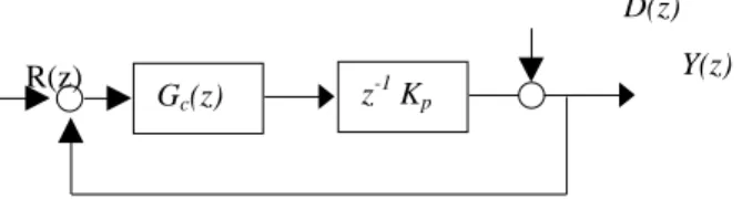
In all cases the control system will have the form shown in Fig. 2.
Fig. 2 Basic CtC Control Loop
The controller Gc (z) will (at this time) be one of two
choices:
Proportional Gc (z) = Kc
Integral Gc (z) = Kc z/(z-1)
A. Stability and Characteristic Response The plant model
Gp(z )=z
−1
Kp (5)
is the same for all processes we expect to consider, the plant reduces to a simple pole at the origin. With proportional control, then, we can show that the stable range of loop gains is given by 0≤KcKp≤1. In addtiion, the expected
response will be oscillatory for all stable gain as the closed-loop root is on the negative real axis of the z-plane.
The integral controller adds a pole at +1 and cancels the plant pole with a zero at the origin. In this case, the stable range is extended to 0≤KcKp≤2 and for 0≤KcKp≤1
the response will be non-oscillatory with a settling time that decreases as KcKp →1., which corresponds to the
closed-loop root approaching the origin of the z-plane.
B. Steady- State Error
Recalling the performance measures defined above, the ability of the CtC system to minimize the target dimension T and the process mean µ is critical. For a stationary dis-turbance modeled as a normal process with constant mean and constant variance, this error can be characterized by the steady-state step input and step disturbance error for the closed-loop system.
For the proportional control there will be a finite step input and step disturbance error given by
ess step = 1 1+KcKp
(6)
Since stability limits KcKp ≤1 we can expect large
er-rors for this controller.
The integral controller will of course have zero steady-state error to both step inputs or disturbances regardless of the loop gain.
C. Variance Reduction
The above are simple classical results that suggest supe-rior performance of the integral controller. Of greater con-cern here, however, is the ability of the CtC control system to reduce the variance of the additive output disturbance. For this analysis we must first more carefully consider our disturbance model.
As previously discussed, two models are appropriate for most manufacturing processes. For processes with fast process dynamics, and with workpiece material changing on each cycle, the events in a disturbance sequence must be independent. For processes with slower dynamics (primar-ily thermal dynamics) there may be some dependence from cycle to cycle.
The uncorrelated noise is simply modeled as a normal identically distributed independent (NIDI) process (or a gaussian white noise process) with mean of µ and variance σ2
. To simulate a dependent or correlated disturbance, this white noise is "colored" with a simple first order filter:
Gf(z )=
1−p z−p
where p =0.8 is chosen for all simulations herein.
1) Variance ratio: White noise, Proportional Control In this case, since each new noise sample is independent of the last, and since the process has at least one time step delay, we expect to see the variance ratio start at 1 and in-crease with gain.
An analysis of this problem is found in Siu[10], who considers not only the steady state variance ratio, but the n result as well. From that analysis it can be shown that the variance: σyn 2 σ2 = 1−K 2n 1−K2 (7) where σy n
2= process output variance at time step n
σ2
= noise variance K = loop gain (KcKp)
From this equation it is apparent that for any value of K the variance of the disturbance will be amplified, as shown in Fig. 3 Gc(z) z -1 Kp D(z) Y(z) R(z)
0.000 2.000 4.000 6.000 8.000 10.000 12.000 0.00 0.20 0.40 0.60 0.80 1.00 Controller Gain, Kc Variance ratio Analytical Matlab simulation
Figure 3 Proportional Control Variance Ratio as n ->∞; Uncorre-lated Disturbances
The transient behavior of Eqn 7 shows an exponential-like rise that reaches steady state at n>12.
2) Variance ratio: Correlated Disturbances with Pro-portional Control
With a correlated disturbance sequence, there is some expectation of variance reduction, since a measure of state dependence exists between successive values of the distur-bance. Closed-form analysis of the case of correlated se-quences is tedious and is not discussed here. However, a simulation of this situation was performed using MATLAB. In this case the CtC system was run for ~5000 transients at each gain level and the average output variance calculated. The result is shown in Fig. 4, and there is indeed a reduc-tion in variance over the range K∈0,0.8 . In fact, the
in-crease in the variance ratio after K = 0.6 can be attributed to the increasingly oscillatory response of the underlying sys-tem, rather than to any steady state noise amplification.
0.000 0.200 0.400 0.600 0.800 1.000 1.200 1.400 1.600 1.800 0.00 0.20 0.40 0.60 0.80 1.00 Controller Gain, Kc Variance ratio
Figure 4 Proportional Control Variance Ratio as n ->∞; Correlated Disturbances
3) Variance ratio: Uncorrelated Disturbances with In-tegral Control
The change to an integral controller has a marked effect on improving steady-state or mean error behavior, but it cannot be expected to reduce variance in the uncorrelated disturbance case any more than in the proportional case. However, since the range of stable gains is great, and tran-sient behavior does improve with gain, it is important to determine the new variance ratio. Again, Siu[10] has per-formed this analysis with the result:
σyn
2
σ2 =1+K⋅
1−(1−K)2( n−1)
2−K (8)
which is plotted in Fig.5
0.000 5.000 10.000 15.000 20.000 25.000 0.000 0.500 1.000 1.500 2.000 Controller Gain, Kc Variance ratio
Time Series Analysis (n=20)
Matlab simulation Frequency Analysis
Figure. 5 Integral Control Variance Ratio as n ->∞; Uncorrelated Disturbances
Here it is noteworthy that variance amplification is mi-nor until K>1, implying a reasonable range of working gains for both transient response performance and variance reduction. However, as gains increase beyond that point, the amplification becomes extreme.
Although Eqn 8 indicates a time dependence for the variance ratio, in fact the transients are over by n=6 for all ranges of gain, and are of little significance here.
4) Variance ratio: Correlated Disturbances with Inte-gral Control
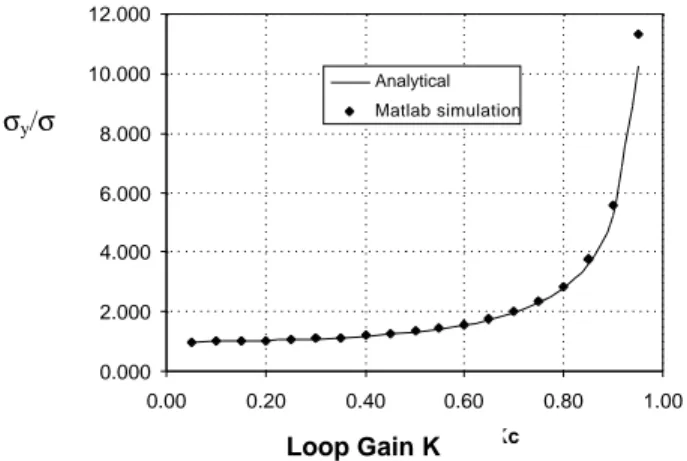
Again the analysis of this situation is beyond the scope of this paper, but Box and Luceno[11] have analyzed the case and show the expected variance reduction. Again us-ing a MATLAB simulation, we can see the large range of useful variance reduction in Fig. 6
Loop Gain K σy/σ Loop Gain K σy/σ Loop Gain K σy/σ
0.000 0.500 1.000 1.500 2.000 2.500 3.000 0.000 0.500 1.000 1.500 2.000 Controller Gain, Kc Variance ratio Analytical Matlab simulation
Figure 6. Variance Ratio for Correlated Disturbances ; Integral Control
D. Summary of CtC Analysis
In this section we have defined a simple process and disturbance model that captures the essential input-output properties of myriad manufacturing processes when sam-pled cycle to cycle. From this model we define two classes of processes: those with uncorrelated disturbances and those with correlated disturbances. It is shown that vari-ance reduction for the former is not possible whereas for the latter it is. In addition, it is shown that an integral con-troller is superior to proportional control of the CtC control loop, primarily owing to its superior error performance.
From this analysis we can also conclude that CtC con-trol, using an integral control law and an appropriately cho-sen loop gain, can center a process on the target value, thereby eliminating mean errors. For a process with uncor-related disturbances, this centering is done at the cost of a slight increase in variance. However, for processes with some correlation in the disturbance, the mean error can be eliminated and variance reduction of up to 50% can be re-alized.
In either case it is important to realize that process ca-pability (Cpk) can be increased for processes subject to
sig-nificant mean drift or shifts, even if they have uncorrelated random disturbance components.
These results are obvious once the model is developed and the problem posed. However, it remains to examine both the validity of the model and the resulting closed-loop system performance. This is presented in a pair of experi-ments designed to look at the two classes of processes: un-correlated and un-correlated.
VI. EXPERIMENTS
To test the results of Section V a series of experiments were performed to implement CtC control. Two processes were chosen to examine different types of process physics and disturbances.
A. Uncorrelated Disturbance Process: Sheet Metal Bending
The simple process of bending is commonly used for many simple sheet metal products. It is well known to be sensitive to material property variations, and is easily im-plemented in a lab setting. For the tests presented here, a simple lab scale 3-point bending apparatus was used, as shown in Fig. 7. The tools are mounted in a simple engine lathe, and the punch is manually moved into the material. The key input is the displacement of the punch Yp into the
material and the output is the included angle of the resulting part. The input was measured by the vernier on the tail-stock of the lathe (with a resolution of 0.001 in.), while the angle is measured with a machinist protractor (with a reso-lution of 5 minutes.)
Figure 7: Setup for Bending Experiments 1) Process Gain
The basic process model is a gain relating the punch po-sition to the output angle. This gain was determined with a series of open-loop experiments on three materials:
• 0.025in thickness steel • 0.020in thickness steel • 0.032in thickness aluminum
These choices allow introduction of different yield stresses, elastic moduli and thicknesses, all of which strongly affect the resulting process gain.
Although the process is known to be non-linear, the model was developed using tests in a small range of output angles so an equivalent linear gain could be determined. A typical result is shown in Fig. 8
Loop Gain K σy/σ Workpiece Punch Die Yp
Figure 8. Gain Determination for 0.025 Steel workpiece The gains found are shown in Table 1
Material Gain Kp (deg/in)
0.025 Steel 151
0.020 Steel 143
0.032 Aluminum 144 Table 1: Process Gains for Bending
2) Closed-Loop Cycle to Cycle Control
To implement CtC control, the angle of each part pro-duced was measured and used to determine the next con-troller output based on the angle error. This represents the one time step delay of the system; the control action is a new punch penetration for the next forming cycle,
To assess the disturbance variance, it was first necessary to perform a number of open-loop runs using fixed punch depths. This was done for each material with 20-30 runs for each test. From these runs it was determined that the open-loop variance was dependent on both material and punch depth. Typical results are shown in Table 2 (The basic measurement repeatability was found to be 0.1°.)
Material Standard Deviation
0.02 Steel 0.161°
0.025 Steel 0.200°· 0.32 Aluminum 0.368°
Table 2: Typical Standard Deviation based on 15-30 Open-Loop Tests
A typical experiment implementing closed-loop control is shown in Fig. 9. Here the process is run open-loop for many cycles, then CtC proportional control with K=0.7 is implemented. As expected, the press variance goes up visi-bly, but the process moves closer to the desired mean value of 35 (although it was at 35.14 open-loop; not a great dis-tance).
Figure 9 Proportional CtC Control of Bending. The target angle was 35°.
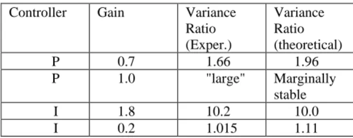
Tests were performed for both proportional and integral control, and transient as well as steady state results were recorded. Some results are shown in Table 3
Controller Gain Variance
Ratio (Exper.) Variance Ratio (theoretical) P 0.7 1.66 1.96 P 1.0 "large" Marginally stable I 1.8 10.2 10.0 I 0.2 1.015 1.11
Table 3 Measured and Theoretical Variance rations for Different Controllers and gains
3) Mean Disturbance Rejection
To simulate a step shift in the mean value of the distur-bance, a sudden change from 0.025in thick steel to 0.020in thick was introduced during CtC operation. This change in thickness will cause a 7.65° shift for a fixed punch dis-placement. The process was taken through the transient and the settling time as well as final steady-state error recorded. As can be seen from Table 4, the results were in compliance with the expected values. for both P and I controllers.
Controller Gain ess exper. ess theo. ts exper. ts theo. P 0.7 4.65 4.29 10 9 I 0.5 0 0 5 5
Table 4 Step Disturbance Rejection (Change of thickness from 0.025 to 0.02 in steel)
The transient results for the I control case with K = 0.5 are shown in Fig. 10
A ramp disturbance was also introduced by adding an offset to the punch position on each cycle. When done at a rate of 1.51°/cycle, it produced divergent results of the P control (as expected) whereas the I controller settled to a y = 151.9x - 156.96 R2 = 1 0 10 20 30 40 50 60 1.1 1.15 1.2 1.25 1.3 1.35 1.4 Punch depth 33.5 34 34.5 35 35.5 36 36.5 0 10 20 30 40 50 60 70 80 90 100 Run number Angle Open-loop Closed-loop
finite error of 3°, exactly as would be predicted for a loop gain of 0.5.
4) Conclusions: Bending Experiments
The experiments with bending have shown close con-formance to the predictions for a process with uncorrelated disturbances. They have also shown the deterministic
dis-Figure 10 Effect of Thickness Change on Integral CtC with K=0.5 turbance (step and ramp) properties of the I controller, and have also confirmed the stability limits predicted by the simple discrete time analysis for this time delay system.
B. Correlated Noise: Injection Molding
For the second experiment, injection molding was cho-sen for several reasons. First, it is a process dominated by thermal time constants, and can be expected to display some correlation between cycles. It is also a far more com-plex "parallel" process that stands at the opposite spectrum in process type from bending. Finally, it typically produces complex parts with one or more critical dimension, and has some well identified input variables.
The part formed was a simple cylinder of ABS and the outer diameter was chosen as the output. (See Fig. 11)
Figure 11 ABS Cylinder Part Forming Using Injection Molding In contrast to bending, the first problem with injection molding is determining which input to use for the experi-ments. The candidates include injection nozzle tempera-ture, hold time (after injection and packing) and injection speed. A 32 experiment was designed to determine which
of these was most sensitive and it was found that hold time was the best input for these test.
1) Process Gain Determinations
Again a series of open-loop experiments were per-formed to determine the process gain relating output dimen-sions (in) to input hold time (sec). Hold time could be re-solved to 0.01 sec on the machine controller and the vernier caliper used to measure the parts had a resolution of 0.0005 in.
From a series of 24 open-loop tests all run after the process had reached thermal equilibrium, the process gain was found to be -1.39 x 10⁻⁴. This means that for the full range of hold times (0-30 sec) we expect only a 0.004in change in part dimension. This is to be expected, however, since the main determinant of part dimension is the tool itself, and this experiment is aimed a making small correc-tions to the basic output dimension.
2) CtC Experiments
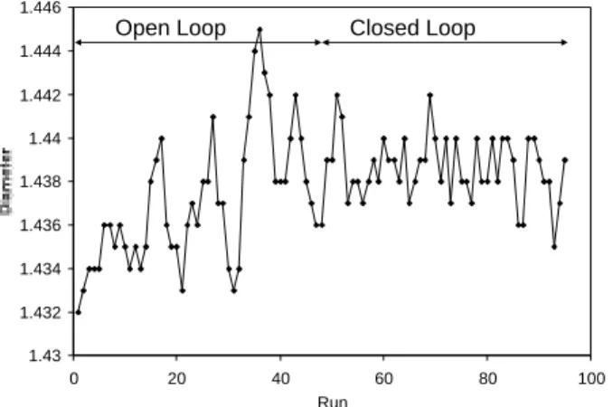
As before, the open-loop variance was first character-ized and then used as a baseline for gauging controller vari-ance reduction. Both P and I controllers were again used, and part dimension feedback was done after each forming cycle. However, owing to the long cooling time of the parts, they were measured "hot" out of the mold. The change in dimension was found to be deterministic and produced a fixed offset that did not influence the variance of the final products.
For the P controller, we expect a reduction in variance, provided the process has some correlation in the distur-bances. In fact, a typical closed-loop run (see fig. 12) shows clearly both the variance reduction and error reduc-tion properties of the controller.
Figure 12 CtC Controller Effect for Injection Molding (P control K = 0.5)
Over a range of reasonable gains for the P controller it was found that the variance ratio was always less than one. For example, when K = 0.2 the variance ratio was 0.74 and when increased to 0.5 it decreased to 0.39. This result fol-lows closely that shown in Fig. 3 (value of 0.7 and 0.5). These results indicate a significant degree of correlation in
26 27 28 29 30 31 32 33 34 35 36 0 5 10 15 20 Run number Material Shift 1.43 1.432 1.434 1.436 1.438 1.44 1.442 1.444 1.446 0 20 40 60 80 100 Run
the disturbance, with the resulting variance reduction using CtC control.
Likewise with the I controller a similar variance reduc-tion was found (e.g. for K=0.2 the variance ratio was 0.4 versus a predicted value of 0.6 from Fig. 4). The error properties of the in controller were harder to assess for this process owing the limited process latitude, and during most step disturbance experiments, the process saturated at the 0.004in change limit, precluding further improvement using hold time as the input.
3) Process Correlation
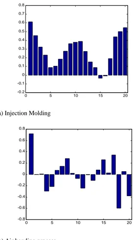
Since distinct variance reduction was observed for the injection molding process the CtC control analysis suggests that the process disturbances must be correlated, that is showing some state dependence from cycle to cycle. To test this finding, the Autocorrelation for the process output when run open-loop was determined. For comparison, the autocorrelation for the bending case was auto calculated. These results are shown in Fig. 13. From these results it appears that there is strong correlation in the 1-5 cycle time range for injection molding, but no real evidence of any correlation in the bending case. This is of course consistent with the variance increase noted in the CtC control for bending. 0 5 10 15 20 -0.2 -0.1 0 0.1 0.2 0.3 0.4 0.5 0.6 0.7 0.8 a) Injection Molding 0 5 10 15 20 -0.8 -0.6 -0.4 -0.2 0 0.2 0.4 0.6 0.8
b) Air bending process
Figure 13 Autocorrelation comparison between open-loop process (left), Process (right)
VII. CONCLUSIONS
The concept of Cycle to Cycle Control has been intro-duced as a simple means of improving process capability using linear discrete time control theory. A simple process model results from assuming that data and control actions can only be taken after the process cycle is complete. Sta-bility limits for the system can be quickly established, and mean error and variance reduction relationships developed. The key observations are:
Regardless of the nature of the output randomness, the mean error can be reduced, producing a more closely cen-tered process. The variance of the process is either slightly increased (for uncorrelated disturbances) or decreased by a significant amount (correlated disturbances) by the CtC control. For both cases the process capability can be im-proved over the open loop (typical of SPC) case.
These results were born out by using CtC on bending and injection molding processes. Not examined here, but detailed by Siu [10] is the ability to determine an optimal gain based on minimizing quality loss.
However, CtC does require knowledge of the often highly variable process gain, and adaptive methods for in-process determination of this quantity should be explored. Also, there are often many coupled output dimensions in a typical product, so multi-variable extension of CtC control would be of great value.
VIII. REFERENCES
[1] Hardt, D.E., "Modeling and Control of Manufacturing Processes: Getting More Involved”, ASME J. of Dynamic Systems Measure-ment and Control, 115, June. 1993, pp 291-300.
[2] Box, G. E. and Kramer, T., "Statistical Process Monitoring and Feedback Adjustment: A Discussion", Technical report, Center for Quality and Productivity Improvement, 1990
[3] Sachs, E. M., Hu, A. and Ingolfsson, A., "Run by Run Process Control: Combining SPC and Feedback Control", IEEE Transaction on Semiconductor Manufacturing, Vol. 8, No. 1, 1995, pp. 26-43 [4] Vander Wiel, S. A. and Tucker, W. T., "Algorithmic Statistical
Process Control: Concepts and an Application", Technometrics, Vol. 34, No. 3, 1992, pp. 286-297
[5] Smith, T. and Boning, D., "A Self-Tuning EWMA Controller Utilizing Artificial Neural Network Function Approximation Tech-niques", International Electronics Manufacturing Symposium, IEMT '96, Oct. 1996
[6] Del Castillo, E. and Hurwitz, A., "Run-to-Run Process Control: Literature Review and Extensions", Journal of Quality Technology, Vol. 29, No. 2, 1997, pp. 184-196
[7] Del Castillo, E., "A multivariate self-tuning controller for run-to-run process control under shift and trend disturbances", IIE Transac-tions, Vol. 28, No. 12, 1996, pp. 1011-1021
[8] Valjavec, M. and Hardt, D.E., “Closed-loop Shape Control of the Stretch Forming Process over a Reconfigurable Tool: Precision Air-frame Skin Fabrication”. Proc. ASME Symposium on Advances in Metal Forming, Nashville, Nov. 1999.
[9] DeVor, R. E., Chang, T., and Sutherland, J. W., Statistical Quality Design and Control: Contemporary Concepts and Methods, Prentice-Hall, Inc., Upper Saddle River, New Jersey, 1992
[10] Siu, T.Z., Cycle to Cycle Feedback Control of Manufacturing Processes, SM Thesis MIT Dept.of ME, Feb. 2001.
[11] Box, G. and Luceño, A., Statistical Control by Monitoring and Feedback Adjustment, John Wiley & Sons, Inc., New York, 1997.