HAL Id: hal-01828312
https://hal.inria.fr/hal-01828312
Submitted on 3 Jul 2018
HAL is a multi-disciplinary open access
archive for the deposit and dissemination of
sci-entific research documents, whether they are
pub-lished or not. The documents may come from
teaching and research institutions in France or
abroad, or from public or private research centers.
L’archive ouverte pluridisciplinaire HAL, est
destinée au dépôt et à la diffusion de documents
scientifiques de niveau recherche, publiés ou non,
émanant des établissements d’enseignement et de
recherche français ou étrangers, des laboratoires
publics ou privés.
Parallel scheduling of DAGs under memory constraints
Loris Marchal, Hanna Nagy, Bertrand Simon, Frédéric Vivien
To cite this version:
Loris Marchal, Hanna Nagy, Bertrand Simon, Frédéric Vivien. Parallel scheduling of DAGs under
memory constraints. IPDPS 2018 - 32nd IEEE International Parallel and Distributed Processing
Symposium, May 2018, Vancouver, Canada. pp.1-10, �10.1109/IPDPS.2018.00030�. �hal-01828312�
Parallel scheduling of DAGs
under memory constraints
Loris Marchal
∗, Hanna Nagy
†, Bertrand Simon
∗and Frédéric Vivien
∗∗CNRS, INRIA, ENS Lyon and University of Lyon, LIP, ENS Lyon, 46 allée d’Italie, Lyon, France †Technical University of Cluj-Napoca, Strada Memorandumului 28, Cluj-Napoca 400114, Romania
Abstract—Scientific workflows are frequently modeled as
Directed Acyclic Graphs (DAG) of tasks, which represent com-putational modules and their dependencies in the form of data produced by a task and used by another one. This formulation allows the use of runtime systems which dynamically allocate tasks onto the resources of increasingly complex computing platforms. However, for some workflows, such a dynamic sched-ule may run out of memory by exposing too much parallelism. This paper focuses on the problem of transforming such a DAG to prevent memory shortage, and concentrates on shared mem-ory platforms. We first propose a simple model of DAGs which is expressive enough to emulate complex memory behaviors. We then exhibit a polynomial-time algorithm that computes the maximum peak memory of a DAG, that is, the maximum memory needed by any parallel schedule. We consider the problem of reducing this maximum peak memory to make it smaller than a given bound by adding new fictitious edges, while trying to minimize the critical path of the graph. After proving this problem NP-complete, we provide an ILP solution as well as several heuristic strategies that are thoroughly compared by simulation on synthetic DAGs modeling actual computational workflows. We show that on most instances we are able to decrease the maximum peak memory at the cost of a small increase in the critical path, thus with little impact on quality of the final parallel schedule.
I. INTRODUCTION
Parallel workloads are often described by Directed Acyclic task Graphs, where nodes represent tasks and edges rep-resent dependencies between tasks. The interest of this formalism is twofold: it has been widely studied in the-oretical scheduling literature [11] and dynamic runtime schedulers (e.g., StarPU [2], XKAAPI [12], StarSs [19], and PaRSEC [5]) are increasingly popular to schedule them on modern computing platforms, as they alleviate the difficulty of using heterogeneous computing platforms. Concerning task graph scheduling, one of the main objectives that have been considered in the literature consists in minimizing the makespan, or total completion time. However, with the increase of the size of the data to be processed, the memory footprint of the application can have a dramatic impact on the algorithm execution time, and thus needs to be optimized [20], [1]. This is best exemplified with an application which, depending on the way it is scheduled, will either fit in the memory, or will require the use of swap mechanisms or out-of-core execution. There are few existing studies that take into account memory footprint when scheduling task graphs, as detailed below in the related work section.
Our focus here concerns the execution of highly-parallel applications on a shared-memory platform. Depending on the scheduling choices, the computation of a given task graph may or may not fit into the available memory. The goal is then to find the most suitable schedule (e.g., one that minimizes the makespan) among the schedules that fit into the available memory. A possible strategy is to design a static schedule before the computation starts, based on the predicted task durations and data sizes involved in the computation. However, there is little chance that such a static strategy would reach high performance: task duration estimates are known to be inaccurate, data transfers on the platform are hard to correctly model, and the resulting small estimation errors are likely to accumulate and to cause large delays. Thus, most practical schedulers such as the runtime systems cited above rely on dynamic scheduling, where task allocations and their execution order are decided at runtime, based on the system state.
The risk with dynamic scheduling, however, is the simul-taneous scheduling of a set of tasks whose total memory requirement exceeds the available memory, a situation that could induce a severe performance degradation. Our aim is both to enable dynamic scheduling of task graphs with memory requirements and to guarantee that at no time during the execution the available memory is exceeded. We achieve this goal by adding fictitious dependencies in the graph to cope with memory constraints: these additional edges will restrict the set of valid schedules and in particular forbid the concurrent execution of too many memory-intensive tasks. This idea is inspired by [21], which applies a similar technique to graphs of smaller-grain tasks. The main difference with the present study is that they focus on homogeneous data sizes: all the data have size 1, which is also a classical assumption in instruction graphs produced by the compilation of programs. On the contrary, our approach is designed for larger-grain tasks appearing in scientific workflows whose sizes are highly irregular.
The rest of the paper is organized as follows:
• We first briefly review the existing work on memory-aware task graph scheduling (Section II).
• We propose a very simple task graph model which both accurately describes complex memory behaviors and is amenable to memory optimization (Section III). • We introduce the notion of the maximum peak
of any (sequential or) parallel execution of the work-flow. We then show that the maximum peak memory of a workflow is exactly the weight of a special cut in this workflow, called the maximum topological cut. Finally, we propose a polynomial-time algorithm to compute this cut (Section IV).
• In order to cope with limited memory, we formally state the problem of adding edges to a graph to decrease its maximum peak memory, with the objec-tive of not harming too much the makespan of any parallel execution of the resulting graph. We prove this problem NP-hard and propose both an ILP formulation and several heuristics to solve it on practical cases (Section V). Finally we evaluate the heuristics through simulations on synthetic task graphs produced by classical random workflow generators (Section VI). The simulations show that the two best heuristics have a limited impact on the makespan in most cases, and one of them is able to handle all studied workflows.
II. RELATEDWORK
Memory and storage have always been a limited param-eter for large computations, as outlined by the pioneering work of Sethi and Ullman [24] on register allocation for task graphs. It was later translated to the problem of scheduling a task graph under memory or storage constraints for scientific workflows whose tasks require large I/O data. Such workflows arise in many scientific fields, such as image processing, genomics, and geophysical simulations. The problem of task graphs handling large data has been identified by Ramakrishnan et al. [20] who introduce clean-up jobs to reduce the memory footprint and propose some simple heuristics. Their work was continued by Bharathi et al. [4] who develop genetic algorithms to schedule such workflows. This problem also arises in sparse direct solvers, as highlighted by Agullo et al. [1] who study the effect of processor mapping on memory consumption for multifrontal methods. In some cases, such as for sparse direct solvers, the task graph is a tree, for which specific methods have been proposed, both to reduce the minimum peak memory [17] and to design memory-aware parallel schedulers [3].
As explained in the introduction, our study is inspired by the work of Sbîrlea at al. [21]. This study focuses on a differ-ent model, in which all data have the same size. They target smaller-grain tasks in the Concurrent Collections (CnC) programming model [6], a stream/dataflow programming language. Their objective is, as ours, to schedule a DAG of tasks under a limited memory. For this, they associate a color to each memory slot and then build a coloring of the data, in which two data with the same color cannot coexist. If the number of colors is not sufficient, additional depen-dency edges are introduced to prevent two data to coexist. These additional edges respect a pre-computed sequential schedule to ensure acyclicity. An extension to support data of different sizes is proposed, which conceptually allocates
several colors to a single data, but is only suited for a few distinct sizes.
In the realm of runtime systems, memory footprint is a real concern. In StarPU, attempts have been made to reduce memory consumption by throttling the task submission rate [22].
Compared to the existing work, the present work studies graphs with arbitrary data sizes, and it formally defines the problem of transforming a graph to cope with a strong memory bound: this allows the use of efficient dynamic scheduling heuristics at runtime with the guarantee to never exceed the memory bound.
III. PROBLEM MODELING
A. Formal description
As stated before, we consider that the targeted applica-tion is described by a workflow of tasks whose precedence constraints form a DAG G = (V,E). Its nodes i ∈ V represent tasks and its edges e ∈ E represent precedence, in the form of input and output data. The processing time necessary to complete a task i ∈ V is denoted by wi. In our model, the
memory usage of the computation is modeled only by the size of the data produced by the tasks and represented by the edges. Therefore, for each edge e = (i , j ), we denote by
me or mi , j the size of the data produced by task i for task
j . We assume that G contains a single source node s and
a single sink node t ; otherwise, one can add such nodes along with the appropriate edges, all of null weight. For the sake of simplicity, we define the following sizes of inputs and outputs of a node i :
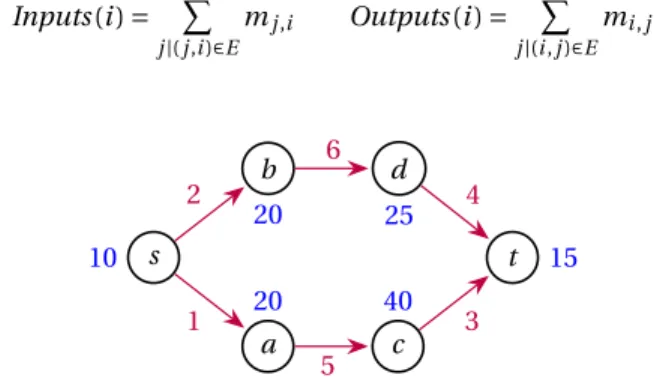
Inputs (i ) = X j |(j,i )∈E mj ,i Outputs (i ) = X j |(i ,j )∈E mi , j s 10 a 20 b 20 c 40 d 25 t 15 1 2 5 6 3 4
Figure 1: Example of a workflow, (red) edge labels represent the size mi , j of associated data, while (blue)
node labels represent their computation weight wi.
We propose here to use a very simple memory model, which might first seem unrealistic, but will indeed prove itself very powerful both to model complex memory behav-iors and to express the peak memory usage. In the proposed model, at the beginning of the execution of a task i , all input data of i are immediately deleted from the memory, while all its output data are allocated to the memory. That is, the amount of used memory Musedis transformed as follows:
This model, called the SIMPLEDATAFLOWMODEL, is ex-tremely simple, and in particular does not allow a task to have both its inputs and outputs simultaneously in memory. However, we will see right below that it is expressive enough to emulate other complex and more realistic behaviors.
Before considering other memory models, we start by defining some terms and by comparing sequential sched-ules and parallel execution of the graph. We say that the data associated to the edge (i , j ) is active at a given time if the execution of i has started but not the one of j . This means that this data is present in memory. A sequential
schedule of a DAG G is defined by an order of its tasks. The memory used by a sequential schedule at a given time is
the sum of the sizes of the active data. The peak memory of such a schedule is the maximum memory used during its execution. A parallel execution of a graph on p processors is defined by:
• An allocation µ of the tasks onto the processors (task
i is computed on processor µ(i));
• The starting times σ of the tasks (task i starts at time
σ(i)).
As usual, a valid schedule ensures that data dependencies are satisfied (σ(j) ≥ σ(i) + wi whenever (i , j ) ∈ E) and that
processors compute a single task at each time step (if
µ(i) = µ(j), then σ(j) ≥ σ(i) + wi or σ(i) ≥ σ(j) + wj). Note
that when considering parallel execution, we assume that all processors use the same shared memory, whose size is limited.
A very important feature of the proposed SIMPLE
-DATAFLOWMODEL is that there is no difference between
sequential schedules and parallel execution as far as memory
is concerned, which is formally stated in the following theorem.
Theorem 1. For each parallel execution (µ,σ) of a DAG G,
there exists a sequential schedule with equal peak memory. Proof. We consider such a parallel execution, and we build
the corresponding sequential schedule by ordering tasks in non decreasing starting time. Since in the SIMPLE -DATAFLOWMODEL, there is no difference in memory be-tween a task being processed and a completed task, the sequential schedule has the same amount of used memory as the parallel execution after the beginning of each task. Thus, they have the same peak memory.
This feature will be very helpful when computing the maximum memory of any parallell execution, in Section IV: thanks to the previous result, it is equivalent to computing the peak memory of a sequential schedule.
B. Emulation of other memory models
1) Classical workflow model: As we explained above, our
model does not allow inputs and outputs of a given task to be in memory simultaneously. However, this is a common behavior, and some studies, such as [15], even consider that in addition to inputs and outputs, some temporary data ti
has to be in memory when processing task i . The memory needed for its processing is then Inputs (i ) + ti+Outputs (i ).
Although this is very different to what happens in the proposed SIMPLEDATAFLOWMODEL, such a behavior can be simply emulated, as illustrated on Figure 2. For all task i , we split it into two nodes i1and i2. We transform all edges (i , j ) by edges (i2, j ), and edges (k, i ) by edges (k, i1). We also add an edge (i1, i2) with an associated data of size
Inputs (i ) + ti+ Outputs (i ). Task i1represents the allocation of the data needed for the computation, as well as the computation itself, and its work is thus wii = wi. Task i2
stands for the deallocation of the input and temporary data and has work wi2= 0.
i wi= 10, ti= 1 2 3 i1 10 i2 0 2 6 3
Figure 2: Transformation of a task as in [15] (left) to the
SIMPLEDATAFLOWMODEL (right).
2) Shared output data: Our model considers that each
task produces a separate data for every of its successors. However, it may well happen that a task i produces an output data d , of size oi ,d, which is then used by several
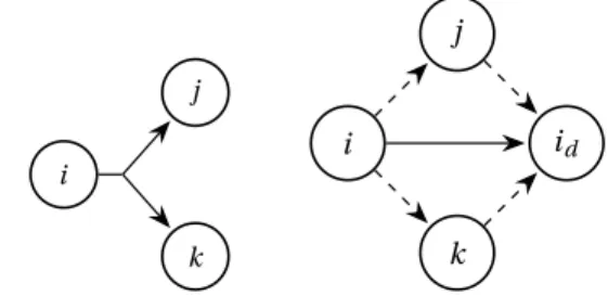
of its successors, and can be freed after the completion of these successors. The output data is then shared among successors, contrarily to what is considered in the SIM -PLEDATAFLOWMODEL. Any task can then produce several output data, some of which can be shared among several successors. Again, such a behavior can easily be emulated in the proposed model, as illustrated on Figure 3.
i j k i j k id
Figure 3: Transformation of a task with a single shared output data (left) into SIMPLEDATAFLOWMODEL(right). The plain edge carries the shared data size, while dashed
edges have null size.
Such a task i with a shared output data will first be transformed as follows. For each shared output data d of size oi ,d, we add a task idwhich represents the deallocation
of the shared data d (and thus has null computation time
wid). An edge of size oi ,d is added between i and id:
mi ,id= oi ,d. Data dependency to a successor j sharing the
output data d is represented by an edge (i , j ) with null data size (mi , j= 0) (if it does not already exist, due to an
other data produced by i and consumed by j ). Finally, for each such successor j , we add an edge of null size ( j , id) to
been used by all the successors sharing it. The following result, whose detailed proof is available in the companion research report [18] states that after this transformation, the resulting graph correctly models the memory behavior.
Theorem 2. Let G be a DAG with shared output data, and
G0 its transformation into SIMPLEDATAFLOWMODEL. There
exists a scheduleσ of G with peak memory at most M if and only if there exists a scheduleσ0of G0 with peak memory at most M .
3) Pebble game: One of the pioneer work dealing with the
memory footprint of a DAG execution has been conducted by Sethi [23]. He considered what is now recognized as a variant of the PEBBLEGAME model. We now show that the proposed SIMPLEDATAFLOWMODEL is an extension of
PEBBLEGAME. The pebble game is defined on a DAG as
follows:
• A pebble can be placed on a node with no predecessor at any time;
• A pebble can be placed on a node if all its predecessors have a pebble;
• A pebble can be removed from a node at any time; • A pebble cannot be placed on a node that has been
previously pebbled.
The objective is to pebble all the nodes of a given graph, using a minimum number of pebbles. Note that the pebble of a node should be removed only when all its successors are pebbled. This is the main difference with our model, where a node produces a different output data for each of its successors. Thus, the PEBBLEGAMEmodel ressembles the model with shared output data presented above, with all data of size one. We thus apply the same transformation and consider that a pebble is a shared output data used for all the successors of a node. In addition, we add a fictitious successor to all nodes without successors. Hence, the pebble placed on such a node can be considered as the data consumed by this successor. Then, we are able to prove that the memory behavior of the transformed graph under
SIMPLEDATAFLOWMODEL corresponds to the pebbling of
the original graph, as outlined by the following theorem (see proof in [18]).
Theorem 3. Let P be a DAG representing an instance of
a PEBBLEGAME problem, and G its transformation into
SIMPLEDATAFLOWMODEL. There exists a pebbling schemeτ
of P using at most B pebbles if and only if there exists a schedule σ0 of G0 with peak memory at most B .
C. Peak memory minimization in the proposed model
The emulation of the PEBBLEGAMEproblem, as proposed above, allows us to formally state the complexity of mini-mizing the memory of a DAG, as expressed by the following theorem.
Theorem 4. Deciding whether an instance of SIMPLE -DATAFLOWMODEL can be scheduled with a memory of limited size is NP-complete.
Proof. The problem of deciding whether an instance of
PEBBLEGAME can be traversed with a given number of
pebbles is NP-complete [23]. Then, thanks to Theorem 3, we know that an instance of PEBBLEGAMEcan be transformed into an instance of SIMPLEDATAFLOWMODEL (with twice as many nodes), which then inherits of this complexity result.
IV. COMPUTING THE MAXIMAL PEAK MEMORY
In this section, we are interested in computing the
maximal peak memory of a given DAG G = (V,E), that is, the
largest peak memory that can be reached by a sequential schedule of G. Our objective is to check whether a graph can be safely executed by a dynamic scheduler without exceeding the memory bound.
We first define the notion of topological cut. We recall that G contains a single source node s and a single sink node t .
Definition 1. A topological cut (S, T ) of a DAG G is a
partition of G in two sets of nodes S and T such that s ∈ S, t ∈ T , and no edge is directed from a node of T to a node of S. An edge (i , j ) belongs to the cut if i ∈ S and j ∈ T . The weight of a topological cut is the sum of the weights of the edges belonging to the cut.
For instance, in the graph of Figure 1, the cut ({s, a, b}, {c, d , t }) is a topological cut of weight 11. In the
SIMPLEDATAFLOWMODEL, the memory used at a given time
is equal to the sum of the sizes of the active output data, which depends solely on the set of nodes that have been executed or initiated. Therefore, the maximal peak memory of a DAG is equal to the maximum weight of a topological cut.
Definition 2. The MAXTOPCUTproblem consists in comput-ing a topological cut of maximum weight for a given DAG.
Note that this problem is more restrictive than computing a maximal cut, which has been proven NP-complete even for DAGs [16], as we enforce that all edges of the cuts are oriented towards the sink node. A polynomial-time solution to the MAXTOPCUT problem can be obtained by solving a linear program and performing a randomized rounding, as we detailed in the companion research report [18]. However, we present here a more direct way of computing the maximum topological cut, through Algorithm 1. We first consider a problem related to the dual version of MAXTOPCUT, which we call MINFLOW:
Definition 3. The MINFLOWproblem consists in computing a flow of minimum value where the amount of flow that passes through each edge is not smaller than its weight.
We recall that the value of a flow f is defined as X
j , (s, j )∈E
fs, j. In this problem the edge weights do not
repre-sent capacities as in a traditional flow, but rather demands: the minimum flow must be larger than these demands on
all edges1. We recall that the MAXFLOW problem consists in finding a flow of maximum value where the amount of flow that passes through each edge is not larger than its weight. Its dual version, the MINCUT problem, consists in computing the st-cut (S, T ) of minimum weight, where s ∈ S and t ∈ T . Note that this cut may not be topological. See [8, Chapter 26] for more details. The MINFLOW problem is described by the following linear program.
min X j | (s,j )∈E fs, j ∀ j ∈ V \ {s, t }, Ã X i | (i ,j )∈E fi , j ! − Ã X k | (j,k)∈E fj ,k ! = 0 ∀(i , j ) ∈ E , fi , j≥ mi , j
We propose in Algorithm 1 an explicit algorithm to resolve the MAXTOPCUT problem. A similar algorithm for a very close problem has been proposed in [7]. We first need an upper bound fmax on the value of the optimal
flow solving the dual MINFLOW problem on G. We can take for instance fmax equal to one plus the sum of the
mi , j’s. The algorithm builds a flow f with a value at least
fmax on all edges. Intuitively, the flow f can be seen as an
optimal flow f∗ solving the MINFLOW problem, on which has been added an arbitrary flow f+. In order to compute
f∗from f , the algorithm explicitly computes f+, by solving a MAXFLOW instance on a graph G+. Intuitively, this step consists in maximizing the flow that can be subtracted from
f∗. Finally, the maximum topological cut associated to the flow f∗ is actually equal to the minimum st-cut of G+ that can be deduced from the residual network induced by f+. We recall that the residual network of G+ induced by f+contains the edge (i , j ) such that either (i , j ) ∈ E and
fi , j+ < m+i , j or ( j , i ) ∈ E and fj ,i+ > 0, as defined for instance in [7].
The complexity of Algorithm 1 depends on two imple-mentations: how we compute the first flow f and how we solve the MAXFLOW problem. The rest is linear in the number of edges. Computing the starting flow f can be done by looping over all edges, finding a simple path from
s to t containing a given edge, and adding a flow going
through that path of value fmax. Note that this method
succeeds because the graph is acyclic, so every edge is part of a simple path (without cycle) from s to t . This can be done in O(|V ||E|). Solving the MAXFLOW problem can de done in O¡|V ||E|log¡|V |2/|E|¢¢ using Goldberg and Tarjan’s algorithm [13]. Therefore, Algorithm 1 can be executed in time O¡|V ||E|log¡|V |2/|E|¢¢.
Theorem 5. Algorithm 1 solves the MAXTOPCUT problem. Proof. First, we show that the cut (S, T ) is a topological cut.
We have s ∈ S and t ∈ T by definition. We now show that no edge exist from T to S in G. By definition of S, no edge exist from S to T in the residual network, so if there exists
1This must not be mistaken with the demands of vertices (i.e., the value
of the consumed flow) as in the Minimum Cost Flow problem.
Algorithm 1: Resolving MAXTOPCUT on a DAG G
1 Construct a flow f for which ∀(i , j ) ∈ E , fi , j≥ fmax,
where fmax= 1 +P(i , j )∈Emi , j (see the description)
2 Define the graph G+ equal to G except that mi , j+ = fi , j− mi , j
3 Compute an optimal solution f+ to the MAXFLOW problem on G+
4 S ← set of vertices reachable from s in the residual
network induced by f+ ; T ← V \ S 5 return the cut (S, T )
an edge ( j , i ) from T to S in G, it verifies fj ,i+ = 0. We then show that every edge of G has a positive flow going through it in f+, which proves that there is no edge from T to S.
Assume by contradiction that there exists an edge (k,`) such that fk,+` is null. Let Sk⊂ V be the set of ancestors
of k, including k. Then, Sk contains s but not t nor ` as
G is acyclic. Denoting Tk= V \ Sk, we get that (Sk, Tk) is a
topological cut as no edge goes from Tkto Sk by definition.
The weight of the cut (Sk, Tk) is at most the value of the
flow f , which is | f |. As f+
k,`= 0, the amount of flow f+
that goes through this cut is at most | f | − fk,`≤ | f | − fmax.
Therefore, the value of f+verifies | f+| ≤ | f | − f
max.
Now, we exhibit a contradiction by computing the amount of flow f+ passing through the cut (S, T ). By definition of (S, T ), all the edges from S to T are saturated in the flow f+: for each edge (i , j ) ∈ E with i ∈ S and j ∈ T , we have fi , j+ = m+i , j= fi , j− mi , j. The value of the flow f+
is equal to the amount of flow going from S to T minus the amount going from T to S. Let ES,T (resp. ET,S) be the
set of edges between S and T (resp. T and S). We have the following (in)equalities: | f+| = Ã X (i , j )∈ES,T fi , j+ ! − Ã X ( j ,i )∈ET,S fj ,i+ ! ≥ Ã X (i , j )∈ES,T ¡ fi , j− mi , j¢ ! − Ã X ( j ,i )∈ET,S fj ,i ! ≥ | f | − Ã X (i , j )∈ES,T mi , j ! > | f | − fmax
Therefore, we have a contradiction on the value of | f+|, so no edge exists from T to S and (S, T ) is a topological cut.
Now, we define the flow f∗ on G, defined by fi , j∗ =
fi , j− fi , j+ ≥ mi , j. We show that f∗ is an optimal solution
to the MINFLOW problem on G. It is by definition a valid solution as f+
i , j ≤ m+i , j = fi , j− mi , j so fi , j∗ = fi , j− fi , j+ ≥
fi , j+ mi , j− fi , j = mi , j. Let g∗ be an optimal solution to
the MINFLOWproblem on G and g+be the flow defined by
gi , j+ = fi , j−gi , j∗. By definition, gi , j∗ ≥ mi , jso gi , j+ ≤ fi , j−mi , j=
m+i , j. Furthermore, we know that g∗i , j≤ fmax because there
exists a flow, valid solution of the MINFLOW problem, of
value P
(i , j )∈Emi , j ≤ fmax: simply add for each edge (i , j )
containing the edge (i , j ). Then, we have gi , j∗ ≤ fmax≤ fi , j so
g+i , j≥ 0 and g+is therefore a valid solution of the MAXFLOW problem on G+, but not necessarily optimal.
So the value of g+is not larger than the value of f+by optimality of f+, and therefore, the value of f∗is not larger than the value of g∗. Finally, f∗ is an optimal solution to the MINFLOWproblem on G.
Now, we show that (S, T ) is a topological cut of maximum weight in G. Let (S0, T0) be any topological cut of G. The total amount of flow of f∗ passing through the edges belonging to (S0, T0) is equal to the value of f∗. As for all (i , j ) ∈ E we have fi , j∗ ≥ mi , j, the weight of the cut
(S0, T0) is not larger than the value of f∗. It remains to show that this upper bound is reached for the cut (S, T ). By the definition of (S, T ), we know that for (i , j ) ∈ (S,T ), we have f+
i , j= mi , j+ = fi , j− mi , j. Therefore, on all these edges,
we have fi , j∗ = fi , j− fi , j+ = mi , j, so the value of the flow f∗
is equal to the weight of (S, T ).
Therefore, (S, T ) is an optimal topological cut.
V. LOWERING THE MAXIMAL PEAK MEMORY OF A GRAPH
In Section IV, we have proposed a method to determine the maximal topological cut of a DAG, which is equal to the maximal peak memory of any (sequential or parallel) traversal. We now move to the problem of scheduling such a graph within a bounded memory M . If the maximal topological cut is at most M , then any schedule of the graph can be executed without exceeding the memory bound. Otherwise, it is possible that we fail to schedule the graph within the available memory. One solution would be to provide a complete schedule of the graph onto a number p of computing resources, which never exceeds the memory. However, using a static schedule can lead to very poor per-formance if the task duration are even slightly inaccurate, or if communication times are difficult to predict, which is common on modern computing platforms. Hence, our objective is to let the runtime system dynamically choose the allocation and the precise schedule of the tasks, but to restrict its choices to avoid memory overflow.
In this section, we solve this problem by transforming a graph so that its maximal peak memory becomes at most
M . Specifically, we aim at adding some new edges to G
to limit the maximal topological cut. Consider for instance the toy example of Figure 1. Its maximal topological cut has weight 11 and corresponds to the output data of tasks a and
b being in memory. If the available memory is only M =
10, one may for example add an edge (d , a) of null weight to the graph, which would result in a maximal topological cut of weight 9 (output data of a and d ). Note that on this toy example, adding this edge completely serializes the graph: the only possible schedule of the modified graph is sequential. However, this is not the case of realistic, wider graphs. We formally define the problem as follows.
Definition 4. A partial serialization of a DAG G = (V,E) for
a memory bound M is a DAG G0= (V, E0) containing all the
edges of G (i.e., E ⊂ E0), on which the maximal peak memory is bounded by M .
In general, there exist many possible partial serializations to solve the problem. In particular, one might add so many edges that the resulting graph can only be processed sequentially. In order to limit the impact on parallel perfor-mance of the partial serialization, we use the critical path length as the metric. The critical path is defined as the path from the source to the sink of the DAG whose total processing time is maximum. By minimizing the increase in critical path when adding edges to the graph, we expect that we limit the impact on performance, that is, the increase in makespan when scheduling the modified graph.
We first show that finding a partial serialization of G for memory M is equivalent to finding a sequential schedule executing G using a memory of size at most M . On the one hand, given a partial serialization, any topological order is a valid schedule using a memory of size at most M . On the other hand, given such a sequential schedule, we can build a partial serialization allowing only this schedule (by adding edge (i , j ) if i is executed before j ). Therefore, as finding a sequential schedule executing G using a memory of size at most M is NP-complete by Theorem 4, finding a partial serialization of G for a memory bound of M is also NP-complete.
However, in practical cases, we know that the minimum memory needed to process G is smaller than M . Therefore, the need to find such a minimum memory traversal adds an artificial complexity to our problem, as it is usually easy to compute a sequential schedule not exceeding M on actual workflows. We thus propose the following definition of the problem, which includes a valid sequential traversal to the inputs.
Definition 5. The MINPARTIALSERIALIZATIONproblem con-sists, given a DAG G = (V,E), a memory bound M, and a sequential scheduleσ of G not exceeding the memory bound, in computing a partial serialization of G for the memory bound M that has a minimal critical path length.
In order to determine the complexity of the MINPAR
-TIALSERIALIZATION problem, we consider its decision
ver-sion, which amounts to finding a partial serialization of a graph G for a memory M with critical path smaller than C P . We prove in the companion research report [18] that this problem is NP-complete, via a reduction from 3-PARTITION. As explained above, this complexity does not come from the search of a sequential traversal with minimum peak memory.
Theorem 6. The decision version of the MINPARTIALSERIAL
-IZATIONproblem is NP-complete, even for independent paths
of length two.
A. Finding an optimal partial serialization through ILP
We present in this section an Integer Linear Program solving the MINPARTIALSERIALIZATION problem. This
for-mulation combines the linear program determining the maximum topological cut and the one computing the critical path of a given graph.
We consider an instance of the MINPARTIALSERIALIZA -TION problem, given by a DAG G = (V,E) with weights on the edges, and a memory limit M . The sequential schedule
σ respecting the memory limit is not required. First, for any
(i , j ) 6∈ E, we set mi , j= 0. We furthermore assume that there
is a single source vertex s and a single target vertex t , as explained above.
We first consider the ei , j variables, which are equal to
1 if edge (i , j ) exists in the associated partial serialization, and to 0 otherwise.
∀(i , j ) ∈ V2, ei , j∈ {0, 1} (1)
∀(i , j ) ∈ E , ei , j= 1 (2)
We need to ensure that no cycle has been created by the addition of edges. For this, we compute the transitive closure of the graph: we enforce that the graph contains edge (i , j ) if there is a path from node i to node j . Then, we know that the graph is acyclic if and only if it does not contain any self-loop. This corresponds to the following constraints:
∀(i , j , k) ∈ V3, ei ,k≥ ei , j+ ej ,k− 1 (3)
∀i ∈ V, ei ,i= 0 (4)
Then, we use the flow variables fi , j, in a way similar
to the formulation of the MINFLOW problem. If ei , j = 1,
then fi , j ≥ mi , j, and fi , j is null otherwise. Now, the flow
going out of s is equal to the maximal cut of the partial serialization, see the proof of Theorem 5, so we ensure that it is not larger than M . Now, note that each fi , j can be
upper bounded by M without changing the solution space. Therefore, Equation (6) ensures that fi , jis null if ei , j is null,
without adding constraints on the others fi , j. This leads to
the following inequalities:
∀(i , j ) ∈ V2, fi , j≥ ei , jmi , j (5) ∀(i , j ) ∈ V2, fi , j≤ ei , jM (6) ∀ j ∈ V \ {s, t }, X i ∈V fi , j− X k∈V fj ,k= 0 (7) X j ∈V fs, j≤ M (8)
This set of constraints defines the set of partial serial-izations of G with a maximal cut at most M . It remains to compute the length of the critical path of the modified graph, in order to formalize the objective. We use the pi
to represent the top-level of each task, that is, their earliest completion time in a parallel schedule with infinitely many processors. The completion time of task s is ws, and the
completion time of another task is equal to its processing time plus the maximal completion time of its predecessors:
ps≥ ws
∀(i , j ) ∈ V2, pj≥ wj+ piei , j
The previous equation is not linear, so we transform it by using W , the sum of the processing times of all the tasks and the following constraints.
∀i ∈ V, pi≥ wi (9)
∀(i , j ) ∈ V2, pj≥ wj+ pi− W (1 − ei , j) (10)
If ei , j is null, then Equation (10) is less restrictive than
Equation (9) as pi < W , which is expected as there is no
edge (i , j ) in the graph. Otherwise, we have ei , j= 1 and the
constraints on pj are the same as above.
Finally, we define the objective as minimizing the top-level of t , which is the critical path of the graph.
Minimize pt (11)
We prove the correctness of this ILP in the companion research report [18].
B. Heuristic strategies to compute a partial serialization
We now propose several heuristics to solve the MINPAR
-TIALSERIALIZATIONproblem. These heuristics are based on
the same framework, detailed in Algorithm 2. The idea of the algorithm, inspired by [21], is to iteratively build a par-tial serialization G0from G. At each iteration, the topological cut of maximum weight is computed via Algorithm 1. If its weight is at most M , then the algorithm terminates, as the obtained partial serialization is valid. Otherwise, another edge has to be added in order to reduce the maximum peak memory. We rely on a subroutine in order to choose which edge to add. In the following, we propose four possible subroutines. If the subroutine succeeds to find an edge that does not create a cycle in the graph, we add the chosen edge to the current graph. Otherwise, the heuristic fails. Such a failure may happen if the previous choices of edges have led to a graph which is impossible to schedule without exceeding the memory.
Algorithm 2: Heuristic for MINPARTIALSERIALIZATION
Input: DAG G, memory bound M , subroutineA Output: Partial serialization of G for memory M
1 while G has a topological cut of weight larger than M
do
2 Compute a topological cut C = (S,T ) of maximum
weight using Algorithm 1
3 if the callA (G,M,C) returns (uT, uS) with no path from node uS to node uT then
4 Add edge (uT, uS) of weight 0 to G 5 else
6 return Failure 7 return the modified graph G
We propose four possibilities for the subroutine
A (G,M,C), which selects an edge to be added to G. They all follow the same structure: two vertices uS and uT are
and uT∈ T and no path exists from uSto uT. The returned
edge is then (uT, uS). For instance, in the toy example of
Figure 1, only two such edges can be added: (c, b) and (d , a). Note that adding such an edge prevents C from remaining a valid topological cut, thus it is likely that the weight of the new maximum topological cut will be reduced.
We first define some classical attributes of a graph: • The length of a path is the sum of the work of all the
nodes is the path, including its extremities;
• The bottom level of an edge (i , j ) or a node i is the length of the longest path from i to t (the sink of the graph);
• The top level of an edge (i , j ) or a node j is the length of the longest path from s (the source of the graph) to j .
We now present the four subroutines. The MINLEVELS heuristic, as well as the two following ones, generates the set P of vertex couples ( j , i ) ∈ T ×S such that no path from
i to j exist. Note that P corresponds to the set of candidate
edges that might be added to G. Then, it returns the couple (uT, uS) ∈ P that optimizes a given metric. MINLEVELS tries
to minimize the critical path of the graph obtained when adding the new edge, by preventing the creation of a long path from s to t . Thus, it returns the couple ( j , i ) ∈ P that minimizes top_level( j ) + bottom_level(i ).
The MAXSIZEheuristic aims at minimizing the weight of the next topological cut. Thus, it selects a couple ( j , i ) such that outgoing edges of i and incoming edges of j contribute a lot to the weight of the current cut. Formally, it returns the coupe ( j , i ) ∈ P that maximizes P
k∈Tmi ,k+Pk0∈Smk0, j
(considering that mi , j= 0 if there is no edge from i to j ).
The MAXMINSIZE heuristic is a variant of the previous heuristic and pursues the same objective. However, it selects a couple of vertices which both contribute a lot to the weight of the cut, by returning the couple ( j , i ) ∈ P that
maximizes min¡P
k∈Tmi ,k , Pk0∈Smk0, j¢.
Finally, the last heuristic is the only one that is guaran-teed to never fail. To achieve this, it relies on a sequential scheduleσ of the graph that does not exceed the memory
M . Such a sequential schedule needs to be precomputed,
and we propose a possible algorithm below.
Given such a sequential scheduleσ, this heuristic, named
RESPECTORDER, always adds an edge ( j , i ) which is
compat-ible with σ (i.e., such that σ(j) ≤ σ(i)), and which is likely to have the smallest impact on the set of valid schedules for the new graph, by maximizing the distanceσ(i)−σ(j) from
j to i inσ. Let uT be the node of T which is the first to be
executed inσ, and uSbe the node of S which is the last to
be executed inσ. First, note that uSmust be executed after
uT inσ, because otherwise, the peak memory of σ will be at
least the weight of C which is a contradiction. The returned couple is then (uT, uS). Note that no path from uSto uT can
exist in the graph if all the new edges have been added by this method. Indeed, all the added edges respect the order
σ by definition. Then, no failure is possible, but the quality
of the solution highly depends on the input scheduleσ.
DAGGEN LIGO MONTAGE GENOME
dense sparse Nb. of test cases 572 572 220 220 220 MINLEVELS 1 12 20 1 0 RESPECTORDER 0 0 0 0 0 MAXMINSIZE 2 5 3 0 0 MAXSIZE 6 12 13 0 17 ILP 26 102
Table I: Number of failures for each dataset
To compute a sequential schedule used as an input for
MINLEVELS, we first assume that any Depth First Search
schedule (DFS), which completes a parallel branch before starting another one, never exceeds the memory bound (in practice we only consider memory bounds that are at least equal to an arbitrary DFS schedule; DFS schedules are known to use very little memory). However, using a DFS for
MINLEVELSis likely to produce a graph with a large critical
path. On the contrary, a Breadth First Search (BFS) schedule is more appropriate, but is not likely to respect the memory bound. We thus use a mix between both schedule. For any
α ∈ [0,1], we define the α-BFSDFS schedule which ranks the tasks by non-decreasing value ofαDFS(i)+(1−α)BFS(i), where DFS(i ) (respectively BFS(i )) is the rank of task i in the DFS (resp. BFS) schedule. It is easy to verify that the
α-BFSDFSschedule respects precedence order, as both DFS and BFS do. The schedule used as an input for MINLEVELS is then computed as follows: we start from the BFS schedule (α = 0), and we increase α until the resulting schedule does not exceed M . In the following experiments, we increment
α by step of 0.05 until we find an appropriate schedule.
VI. SIMULATION RESULTS
We now compare the performance of the proposed heuristics through simulations on synthetic DAGs. All heuristics are implemented in C++ using the igraph library. We generated the first dataset, named DAGGEN, using the DAGGEN software [25]. This dataset, described in [18], has already been used to model workflows in the scheduling literature [14], [10]. We split it in two parts (sparse and dense) depending on the density of edges in the graphs, as this parameter leads to significant differences in the results. The other datasets represent actual applications and have been generated with the Pegasus Workflow Generator [9]. We consider three datasets, named LIGO, MONTAGE, and
GENOME, each containing 20 graphs of 100 nodes (see [18]
for details on how to adapt these graphs to our model). The heuristics have been simulated for eleven memory bounds per DAG, evenly spread between two bounds. The smallest bound corresponds to the memory required for a DFS schedule, while the largest bound corresponds to the maximal peak memory of the DAG. In the results, a normalized memory of 0 corresponds to the lowest bound, while 1 corresponds to the largest bound. Note that the ratio between the largest and the smallest bound ranges
1 2 3 4 5 0 0.1 0.2 0.3 0.4 0.5 0.6 0.7 0.8 0.9 1
Normalized memory bound
Normalized
critical
path
Heuristic MinLevels RespectOrder MaxMinSize MaxSize
Figure 4: Critical path length obtained by each method for the sparse DAGGEN dataset.
from 1.2 to 2.5 for the DAGs generated by DAGGEN, and from 5 to 21 for the one of Pegasus (see details in [18]).
In order to assess the performance of the heuristics, we first examine the critical path length of the obtained partial serialization. We first normalize each critical path by the critical path of the original graph. Therefore, for the largest memory bounds, the original graph being itself a valid partial serialization, all the normalized critical paths equal 1. When a method fails, we say that the critical path achieved is infinite. Failure rates are reported in Table I.
We plot the results obtained for the sparse and dense
DAGGEN dataset in Figures 4 and 5 respectively. For each
heuristic and memory bound, we display the 108 results as a Tukey boxplot. The box presents the median, the first and third quartiles. The whiskers extend to up to 1.5 times the box height, and points outside are plotted individually. The first trend that can be observed, is that, as expected, the lower the memory bound, the larger the critical path. The difference between the minimal and the maximal memory
1.0 1.5 2.0 2.5 3.0 3.5 0 0.1 0.2 0.3 0.4 0.5 0.6 0.7 0.8 0.9 1
Normalized memory bound
Normalized
critical
path
Heuristic MinLevels RespectOrder MaxMinSize MaxSize ILP
Figure 5: Critical path length obtained by each method for the dense DAGGENdataset.
bound is smaller for dense graphs. Therefore, it is logical that the heuristics lead to a larger increase of the critical path in sparse graphs. Comparing the heuristics, we can see that MINLEVELSclearly outperforms the other ones for any value of the memory bound. Then, RESPECTORDERobtains better performance than MAXMINSIZEand MAXSIZE, except when the memory bound is the lowest, where these three heuristics are comparable. The results are widely spread as the graphs differ in several parameters. We remark therefore that MINLEVELS is highly robust considering the variety of the graphs. On this dataset, we have also computed the optimal solution by using the Integer Linear Program presented in Section V. We implemented the ILP using CPLEX with a time limit of one hour of computation on a standard laptop computer (8 cores Intel i7). When it exceeded the time limit, we assume a failure. This happens on sparse graphs, especially for low memory bounds, which is why it is omitted on Figure 4.
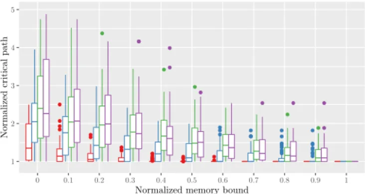
We plot the results obtained for the LIGO dataset on Figure 6, showing the critical path lengths achieved by each heuristic for each memory bound. The similar structure of all graphs in this dataset explains that the results lie in a smaller interval. The hierarchy of the heuristics is the same as in the DAGGEN dataset: MINLEVELS presents the best performance, RESPECTORDERleads to slightly longer criti-cal paths, and MAXSIZE and MAXMINSIZE achieve similar results, several times higher than the first two heuristics. Note that for the lowest memory bound, MINLEVELS never succeeds in this dataset (hence, it does not appear in the plot), MAXSIZE also presents a high failure rate, whereas
RESPECTORDERand MAXMINSIZEhave comparable results.
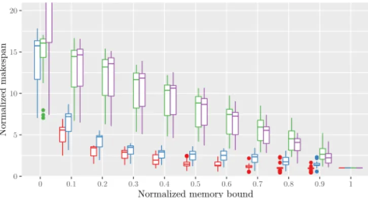
Another criterion we use to compare the heuristics con-sists in evaluating the makespan achieved by a simple scheduling heuristic on the partial serialization returned by each heuristic on a simulated platform. The chosen scheduling heuristic is the traditional list-scheduling al-gorithm, in which whenever a task terminates, the
avail-0 5 10 15 20 0 0.1 0.2 0.3 0.4 0.5 0.6 0.7 0.8 0.9 1
Normalized memory bound
Normalized
critical
path
Heuristic MinLevels RespectOrder MaxMinSize MaxSize
Figure 6: Critical Path length obtained by each method for the LIGO dataset.
0 5 10 15 20 0 0.1 0.2 0.3 0.4 0.5 0.6 0.7 0.8 0.9 1
Normalized memory bound
Normalized
mak
espan
Heuristic MinLevels RespectOrder MaxMinSize MaxSize
Figure 7: Makespan obtained by each method for the LIGO dataset.
able task with the highest bottom level is executed. This corresponds to the well-known HEFT scheduler [26] when adapted to dynamic schedulers, as for example done in the dmda scheduler of StarPU [2]. Figure 7 presents the sim-ulation on 5 processors. Except the slightly more scattered results, the ranking of the heuristics is very similar to the one obtained with the critical path. Therefore, even if the final objective is to obtain a graph that we can schedule within a small makespan, our objective of minimizing the critical path is completely relevant.
In the companion research report [18], we present the results for the MONTAGEand GENOMEdatasets, which show the same trends as the LIGO dataset.
VII. CONCLUSION
In this paper, we have focused on lowering the memory footprint of task graphs representing computational work-flows. As we recognize the need for dynamic schedules (such as in runtime systems), we have focused on the transformation of the graphs prior to the scheduling phase. Adding fictitious edges that represent “memory depen-dencies” prevents the scheduler to run out of memory. After formally modeling the problem, we have shown how to compute the maximal peak memory of a graph, we have proven the problem of adding edges to cope with limited memory while minimizing the critical path to be NP-complete, and proposed both an ILP formulation of the problem and several heuristics. Our simulations show that our best heuristics, RESPECTORDER and MINLEVELS, either never fail, or are able to limit the memory footprint with limited impact of the parallel makespan for most task graphs. Our future work consists in implementing the proposed heuristics in a runtime system and evaluate them on actual graphs.
REFERENCES
[1] E. Agullo, P. R. Amestoy, A. Buttari, A. Guermouche, J. L’Excellent, and F. Rouet. Robust memory-aware mappings for parallel multifrontal factorizations. SIAM J. Scientific Computing, 38(3), 2016.
[2] C. Augonnet, S. Thibault, R. Namyst, and P.-A. Wacrenier. StarPU: a unified platform for task scheduling on heterogeneous multicore architectures. Concurrency and Computation: Practice and Experience, 23(2):187–198, 2011.
[3] G. Aupy, C. Brasseur, and L. Marchal. Dynamic memory-aware
task-tree scheduling. In Proc. of the Int. Par. and Dist. Processing
Symposium (IPDPS), pages 758–767. IEEE, 2017.
[4] S. Bharathi and A. Chervenak. Scheduling data-intensive workflows on storage constrained resources. In Proc. of the 4th Workshop on
Workflows in Support of Large-Scale Science (WORKS’09). ACM, 2009.
[5] G. Bosilca, A. Bouteiller, A. Danalis, M. Faverge, T. Herault, and J. J. Dongarra. PaRSEC: Exploiting heterogeneity for enhancing scalability.
Computing in Science & Engineering, 15(6):36–45, 2013.
[6] Z. Budimli´c, M. Burke, V. Cavé, K. Knobe, G. Lowney, R. Newton, J. Palsberg, D. Peixotto, V. Sarkar, F. Schlimbach, et al. Concurrent collections. Scientific Programming, 18(3-4):203–217, 2010.
[7] E. Ciurea and L. Ciupalâ. Sequential and parallel algorithms for
minimum flows. Journal of Applied Mathematics and Computing, 15(1):53–75, 2004.
[8] T. H. Cormen, C. E. Leiserson, R. L. Rivest, and C. Stein. Introduction
to Algorithms, Third Edition. The MIT Press, 3rd edition, 2009.
[9] R. F. Da Silva, W. Chen, G. Juve, K. Vahi, and E. Deelman. Community resources for enabling research in distributed scientific workflows. In
10th Int. Conf. on e-Science, volume 1, pages 177–184. IEEE, 2014.
[10] F. Desprez and F. Suter. A bi-criteria algorithm for scheduling parallel task graphs on clusters. In CCGrid, pages 243–252. IEEE, 2010. [11] M. Drozdowski. Scheduling parallel tasks – algorithms and
com-plexity. In J. Leung, editor, Handbook of Scheduling. Chapman and Hall/CRC, 2004.
[12] T. Gautier, X. Besseron, and L. Pigeon. KAAPI: A thread scheduling runtime system for data flow computations on cluster of multi-processors. In International Workshop on Parallel Symbolic
Com-putation, pages 15–23, 2007.
[13] A. V. Goldberg and R. E. Tarjan. A new approach to the maximum flow problem. In Proceedings of ACM STOC, pages 136–146, 1986. [14] S. Hunold. One step toward bridging the gap between theory and
practice in moldable task scheduling with precedence constraints.
Concurrency and Computation: Practice and Experience, 27(4):1010–
1026, 2015.
[15] M. Jacquelin, L. Marchal, Y. Robert, and B. Uçar. On optimal tree traversals for sparse matrix factorization. In Proc. of the Int. Par. &
Dist. Processing Symposium (IPDPS), pages 556–567. IEEE, 2011.
[16] M. Lampis, G. Kaouri, and V. Mitsou. On the algorithmic effective-ness of digraph decompositions and complexity measures. Discrete
Optimization, 8(1):129–138, 2011.
[17] J. W. H. Liu. An application of generalized tree pebbling to sparse matrix factorization. SIAM J. Alg. Discrete Methods, 8(3):375–395, 1987. [18] L. Marchal, H. Nagy, B. Simon, and F. Vivien. Parallel scheduling of DAGs under memory constraints. Research Report RR-9108, INRIA, Oct. 2017. https://hal.inria.fr/hal-01620255.
[19] J. Planas, R. M. Badia, E. Ayguadé, and J. Labarta. Hierarchical task-based programming with StarSs. IJHPCA, 23(3):284–299, 2009. [20] A. Ramakrishnan, G. Singh, H. Zhao, E. Deelman, R. Sakellariou,
K. Vahi, K. Blackburn, D. Meyers, and M. Samidi. Scheduling data-intensiveworkflows onto storage-constrained distributed resources. In
CCGrid’07, pages 401–409, 2007.
[21] D. Sbîrlea, Z. Budimli´c, and V. Sarkar. Bounded memory scheduling of dynamic task graphs. In Proc. of PACT, pages 343–356. ACM, 2014. [22] M. Sergent, D. Goudin, S. Thibault, and O. Aumage. Controlling the memory subscription of distributed applications with a task-based runtime system. In Proc. of IPDPS Workshops, pages 318–327. IEEE, 2016.
[23] R. Sethi. Complete register allocation problems. SIAM journal on
Computing, 4(3):226–248, 1975.
[24] R. Sethi and J. Ullman. The generation of optimal code for arithmetic expressions. Journal of the ACM, 17(4):715–728, 1970.
[25] F. Suter. Daggen: A synthetic task graph generator. https://github. com/frs69wq/daggen.
[26] H. Topcuoglu, S. Hariri, and M. Y. Wu. Performance-effective and low-complexity task scheduling for heterogeneous computing. IEEE