Convex optimization and machine learning for scalable verification and control

(1)

Convex Optimization and Machine Learning for

Scalable Verification and Control

by

Shen Shen

Submitted to the Department of Electrical Engineering and Computer

Science

in partial fulfillment of the requirements for the degree of

Doctor of Philosophy

at the

MASSACHUSETTS INSTITUTE OF TECHNOLOGY

September 2020

© Massachusetts Institute of Technology 2020. All rights reserved.

Author . . . .

Department of Electrical Engineering and Computer Science

July 31, 2020

Certified by. . . .

Russ Tedrake

Professor of Electrical Engineering and Computer Science

Thesis Supervisor

Accepted by . . . .

Leslie A. Kolodziejski

Professor of Electrical Engineering and Computer Science

Chair, Department Committee on Graduate Students

(2)

(3)

Convex Optimization and Machine Learning for Scalable

Verification and Control

by

Shen Shen

Submitted to the Department of Electrical Engineering and Computer Science on July 31, 2020, in partial fulfillment of the

requirements for the degree of Doctor of Philosophy

Abstract

Having scalable verification and control tools is crucial for the safe operation of highly dynamic systems such as complex robots. Yet, most current tools rely on either convex optimization, which enjoys formal guarantees but struggles scalability-wise, or black-box learning, which has the opposite characteristics. In this thesis, we address these contrasting challenges, individually and then via a rapprochement.

First, we present two scale-improving methods for Lyapunov-based system veri-fication via sum-of-squares (SOS) programming. The first method solves composi-tional and independent small programs to verify large systems by exploiting natural, and weaker than commonly assumed, system interconnection structures. The second method, even more general, introduces novel quotient-ring SOS program reformu-lations. These programs are multiplier-free, and thus smaller yet stronger; further, they are solved, provably correctly, via a numerically superior finite-sampling. The achieved scale is the largest to our knowledge (on a 32 states robot); in addition,

tighter results are computed 2–3 orders of magnitude faster.

Next, we introduce one of the first verification frameworks for partially observable systems modeled or controlled by LSTM-type (long short term memory) recurrent neural networks. Two complementary methods are proposed. One introduces novel integral quadratic constraints to bound general sigmoid activations in these networks; the other uses an algebraic sigmoid to, without sacrificing network performances, arrive at far simpler verification programs with fewer, and exact, constraints.

Finally, drawing from the previous two parts, we propose SafetyNet, which via a novel search-space and cost design, jointly learns readily-verifiable feedback controllers and rational Lyapunov candidates. While leveraging stochastic gradient descent and over-parameterization, the theory-guided design ensures the learned Lyapunov candi-dates are positive definite and with “desirable” derivative landscapes, so as to enable direct and “high-quality” downstream verifications. Altogether, SafetyNet produces sample-efficient and certified control policies—overcoming two major drawbacks of reinforcement learning—and can verify systems that are provably beyond the reach of pure convex-optimization-based verifications.

Thesis Supervisor: Russ Tedrake

(4)

(5)

Acknowledgments

I am deeply grateful to my advisor Russ Tedrake for his support and guidance — his investment in me, his interest and encouragement, his tremendous patience and faith, his technical inputs and constructive advices, his way of developing my skills and perspectives, and his overall help turning my inkling of what is research into the work presented here. I feel fortunate for having his deep insight, broad vision, and acute sense of technical substance versus mere cleverness to draw on. More broadly, his work ethic, open-mindedness, and disciplined and healthy lifestyle, still to this day, inspire me day-to-day. It has truly been an honor and a pleasure to work with Russ.

I would like to thank my thesis committee: Sasha Megretski and Pablo Parrilo. The bi-weekly meetings with them and Russ over the past two years have been nothing short of inspiration. I fondly remember zigzagging with them to fit ideas in between trivial and impossible, and how their quick pointers easily nudge me out of deadzones. Their debates and critique sessions reflect a balanced taste and historical perspective that took many years of effort to develop, and to be able to simply feed off those is a privilege I deeply cherish. Their questions and advices helped improve the clarity of many parts in this thesis. I would like to particularly thank Pablo for his direct inputs to Chapter 4 and Sasha for his inputs to Chapter 3.

I would also like to thank all the Robot Locomotions Group members for making the lab so stimulating and collaborative. Hongkai Dai, Robin Deits, and Twan Koolen effectively guided me into the lab. Knowledgeable and patient, they introduced to me the tools, problems, and culture in the lab, and greatly flattened the learning curve for me. They, along with Russ, happen to all be programming wizards, and imparted to me many good software engineering practices as well. I would like to thank Sadra Sadradinni for leading a collaboration on a verification paper; and thank him and Tobia Marcucci and Jack Umenberger for many helpful control and optimization-oriented discussions, and Yunzhu Li and Lucas Manuelli for many learning-related ones. I would also like to thank Tao Pang, Greg Izatt, and Wei Gao for keeping us

(6)

informed of the advancements in mechanics, manipulation, and computer vision. And thanks to Mieke Moran, Stacie Ford (from TRI), and Gretchen Jones for being so awesome at supporting our lab.

Over the years, thanks to the help of many, I was fortunate to get familiar with var-ious topics that would otherwise be too time-consuming or peripheral for me to invest in. In particular, I would like to thank Diego Cifuentes for tutorial and many helpful discussions on algebraic geometry, which are instrumental for Chapter 4. Thanks to Osbert Bastani for many discussions on safe reinforcement learning via our collab-oration, which helped accelerate my overall understanding of the field. Thanks to Aleksander Madry for initiating the CDML weekly meetings, which demystified for me many statistical and causal learning researches, and brought to my attention the studies of over-parameterization which later inspired a part of the designs in Chap-ter 6. Thanks to Hadas Kress-Gazit and Jacopo Banfi for many infrastructure and perception-in-the-loop discussions for the Periscope MURI. Thanks to Micah Fry for many interesting conversations on transferring the work to the test-bed in the Lincoln Lab, which taught me quite a lot about ground vehicle hardwares.

Thanks to all the professors whom I have had the chance to TA for: Devavrat Shah, David Sontag, Suvrit Sra, Jeff Lang, Karl Berggren, Gerry Sussman, and Qing Hu. Teaching has always been a passion of mine. To be able to get suggestions, tips, and directions from them to more confidently and effectively engage my class for the teaching, and, moreover, to be able to get a greater appreciation of the tech-nical material through these teaching opportunities for my own learning, it is deeply rewarding.

Special thanks to my graduate counselor Asu Ozdaglar. Prior to working with Russ, my PhD journey was rather bumpy, when I would often feel overwhelmed (sometimes even lost) by all the possible research labs to join and classes to take. Asu generously shared her time, experience, and wisdom, and encouraged and guided me back to the right track.

My master’s years were spent at the Media Lab, and I would like to take this opportunity to thank my then advisor Andrew Lippman. His eloquence, wit, wisdom,

(7)

and humor made my time at the lab not only fulfilling but enjoyable. I learned the importance of crafting an argument and the art of sales from losing many casual and fun debates to Andy. I am also grateful to Andy for connecting with Chess Grandmaster Maurice Ashley for collaboration; I feel very fortunate to have the chance to work on a project that mixes teaching, chess, software engineering, and social studies, all of which I truly enjoy.

This is also a fitting opportunity to thank my teachers and friends from my under-grad years at the Harbin Institute of Technology. My professors, in both Aero/Astro and English Literature departments, helped prepare me for transitioning into this academically and culturally different post-grad life. I would like to particularly thank Huijun Gao and Lixian Zhang for providing for me my first research home, and Ye Zhao for leading the project that would turn into my first paper. I would also like to thank Yibo, Yue, Peng, and Dan for being wonderful friends through those years and for the kind consolation to me and my mom when my dad suddenly passed away.

Thanks to my friends at MIT, Ying, Mitra, Lei, Yehua, and Ying-zong. You are the big brothers and sisters I never had; thank you for all your life and career advices, for putting up with my “shen-anigans” and laughing at my dumb jokes.

Thanks to my maternal grandparents for nurturing my love of comedy, literature, and opera. At times of inevitable frustration and anxiety, like now, as I write this thesis amidst this pandemic, those have been a great escape and reminder of the broader beauty in the world.

To my mother, thank you for just being you, strong, caring, and independent. Thank you also for always being there for me, for being a constant joy in my life, and for showing me how to love life. To my late father, I do wish you were alive to share this journey and moment, but I like to believe that you knew already I would have enjoyed what I experienced at MIT. After all, it was the fun we had playing with Legos, skateboards, and RC planes that sparked this dream in engineering. Thank you and love you, mom and dad. I am blessed to be your daughter.

(8)

(9)

List of Figures

2-1 IQC tutorial example. For both systems, the dynamics is 𝑥+ _{= (𝑥 +}

𝑓 (𝑥))/3where 𝑓(𝑥) is a difference equation for system I and a difference

inclusion for system II. . . 27

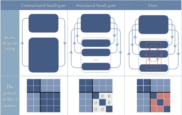
3-1 Our setup compared with the unstructured and structured small-gain setup. Our setup takes advantage of the ‘weak’ internal interconnec-tion, thus achieve a ‘balance’ between the unstructured and structured

cases. . . 38

3-2 Sparsity pattern of three LMIs for 𝑀 = 8 example . . . 38

4-1 The proposed method significantly reduces both formulation and com-putation overhead. One resulting improvement is visualized above on the ROA approx. of the Van der Pol. Traditional methods typically involve conditions on, e.g., the set of all states enclosed within the yellow line, and solve an optimization globally. Our method,

prov-ably correct and less conservative, only needs to examine few random

samples, shown as blue dots, on the yellow line. . . 52

4-2 Standard SOS-based verification pipeline and the traditional overhead. We follow the same pipeline but use different ingredients throughout. Thus, unlike most scale-improving methods that are SDP-oriented, we

reduce all these overhead. . . 54

(14)

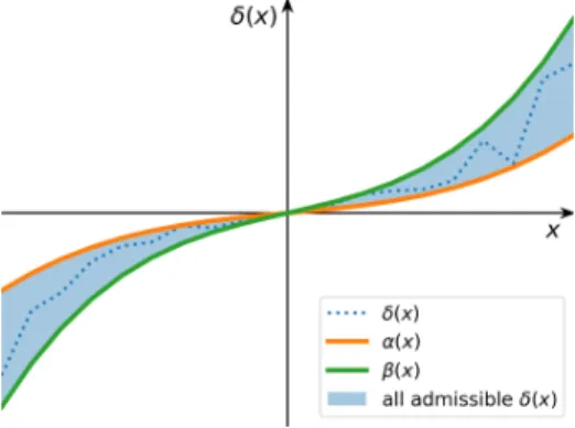
4-4 Generalized Lur’e type sector uncertainty. 𝛼(𝑥) and 𝛽(𝑥), both poly-nomial, define the “boundaries” of the sector; the uncertainty 𝛿(𝑥) can

take any function “in between”. . . 63

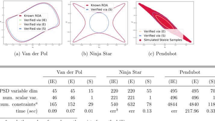
4-6 ROA approximations of polynomial systems. Qualitatively, for Van-derPol, all three programs return identical result; for Ninja star, only the proposed method (S) succeeds; for Pendubot, the proposed method is tighter. . . 69

4-7 Path-tracking Dubins vehicle in the virtual error frame . . . 70

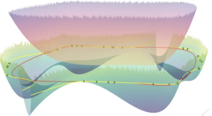
4-8 Robust ROA analysis for Dubins vehicle tracking a path of varying curvature. The yellow outer tube corresponds to 𝑘𝑣 = 0.8 (straighter path). The green inner-tube corresponds to 𝑘𝑣 = 1.2. The inner-tube is also the robust ROA for any 𝑘𝑣 varying within the given range. The red dots are counter-examples that do not converge to the origin; they show the tightness of the approximation. . . 71

4-9 SDP complexity as the number of links in the N-link on cart system Figure 4-5 grows. Note the log-scale. . . 72

5-1 Standard verification setup for FFNN (left) and direct application of this idea to an unrolled RNN(right) . . . 78

5-2 Our Method I relies on a relaxation for general activations in the sig-moidal family; hyperbolic tangent is used here for illustration. The relaxation is the conjunction of four quadratic constraints and the key ingredient in our control theory and convex optimization powered ver-ification framework. . . 79

5-3 The training process. . . 83

5-4 The verification objective. . . 84

(15)

5-6 Two shifted sector conditions and their conjunction. The shift

con-stants 𝛼 and 𝛽 can be arbitrarily chosen as long as 𝛼 = 𝛽 − tanh−1_(𝛽);

the plot corresponds to the choice of 𝛽 = 0.77, and 𝛼 = 0.77 −

tanh−1(0.77) . . . 87

5-7 Hierarchical conjunctions of various IQCs. . . 87

5-8 Canonical friction model in mechanical systems, where 𝐹 is an applied force, 𝑓 is the friction force, 𝜇 is the dynamic coefficient of friction,

𝑛 is the magnitude of the normal force. Such nonlinearity can be

similarly handled via the proposed QCs/IQCs. Figure taken online

from Quora.com. . . 89

5-9 tanh(𝑥) versus the proposed AlgSig nonlinear activation . . . 91

5-10 True output 𝑦 v.s. predicated output ˆ𝑦 trajectories, sampled from the

test data set. . . 95

5-11 Verified samples v.s. the true ROA. . . 96

5-12 Verified ellipsoid ROA for the closed-loop double integrator system

using RNN as a partial state feedback controller . . . 98

5-13 The verified ROA and the sampled stable initial states for the satellite

plant controlled by RNN with AlgSig activation. . . 99

5-14 ReLU and polynomial and rational approximations [74] . . . 100 5-15 The fast InvSqrt() source code . . . 101 6-1 The double descent risk curve proposed by Belkin et al. [11]. It

incor-porates the U-shaped risk curve (i.e., the “classical” regime) together with the observed behavior from using high capacity function classes (i.e., the “modern” interpolating regime). . . 114 6-2 Virtual error frame for Dubins path tracking . . . 118 6-3 Rational candidate 𝑉 and the corresponding ˙𝑉 for system Eq. 6.4 . . 119 6-4 Contour of the rational candidate 𝑉 and the corresponding ˙𝑉 for

(16)

6-5 𝑉 and ˙𝑉 of the pendulum plant (mass 𝑚 = 1, length 𝑙 = 0.5, damping

𝑏 = 0.1 and gravity 𝑔 = 9.81) controlled by the sampling-generated

feedback controller 𝜋(𝑥) = 6.8679447 sin(𝜃) + 0.36002526(cos(𝜃) + 1) − 4.646804 ˙𝜃. Both 𝑉 and ˙𝑉 are recast back from the [𝑠, 𝑐, ˙𝜃] coordinate to the original [𝜃, ˙𝜃] for plotting. . . 122 6-6 Forward simulations of 30 random initial conditions for the Pendulum

Recast plant with sampling-based trigonometric feedback controller. . 122 6-7 Forward simulations of 30 random initial conditions for the Dubins

Recast plant with sampling-based trigonometric feedback controller. . 123 6-8 Eigenvalues of four 9-by-9 Gram matrix using different factorization

sizes. For example, the Gram matrix 𝑄𝑎in plot (a) is constructed from

the factorization 𝑄 = 𝐿′

1𝐿1 where 𝐿1 ∈ R9×9, the one in plot (b) 𝑄𝑏

is constructed from the factorization 𝑄 = 𝐿′

1𝐿′2𝐿2𝐿1 where 𝐿1 ∈ R9×9,

and 𝐿1 ∈ R9×27, and similarly for the next two plots. . . 124

6-9 Average entropy over 1,000 Gram matrix for each fixed parameteriza-tion scheme . . . 125

(17)

List of Tables

3.1 Run-time and success rates for LTI systems . . . 43

3.2 Run-time comparison for Lotka-Volterra system . . . 44

4.1 Numerical comparison of three methods for ROA verification. . . 69

4.2 Numerical results of the ROA problem with different number of links

on the cart. . . 72

5.1 Accuracies [%] on benchmark datasets for different RNN architectures. All networks have a single hidden layer of 128 units. “Janet w. AlgSig (swap)” are pre-trained Janet networks with all their tanh activation function swapped with the AlgSig activation, while keeping all weights (therefore the arguments in the activation as well) fixed. “Janet w. AlgSig (retrain)” are the swapped models with weights updated from further training. The means and standard deviations from 10

(18)

(19)

Chapter 1 Introduction

The recent years witnessed a momentous growth of impressive robotics applications: obstacle-avoiding drones, back-flipping humanoids, Rubiks-solving and Lego-playing robotic hands, (semi)autonomous cars, not to mention the “purpose-built robots” for food delivering or warehouse packing, which were once a fantasy and now a somewhat mundane reality.

While a unifying theme of “safely and more reliably perform more dexterous and complex real-world tasks” clearly emerges from these advancements, under the hood, such progress in verification and control is made possible by two fundamentally dif-ferent approaches. One approach is deeply rooted in control theory and convex op-timization, as represented by Lyapunov theory and sum-of-squares (SOS) programs; and the other is data-driven, as represented by deep neural networks and supervised or reinforcement learning.

At the heart of the co-existence of the two approaches are their contrasting pros and cons. The optimization-based offer provable performance guarantee, but the core assumption of convexity restricts their scale and generality. On the contrary, despite the ever-increasing popularity and stellar empirical performance, analysis of learning-based methods is elusive due to the models’ black-box nature.

(20)

1.1 Contribution

In this thesis, we address these contrasting challenges of the two approaches, first individually and then via a rapprochement. In particular, we propose to improve the scalability of the optimization-based; bridge the analytical gap of the learning-based; and design a balanced (structured) mixture of the two.

First in Part I, we present two methods to address the well-acknowledged scal-ability challenge for Lyapunov-based stscal-ability verification via sum-of-squares (SOS) programming. The first method exploits that large-scale systems are often natural interconnections of smaller subsystems, and solves independent and compositional small programs to verify the large systems. Compared with existing compositional methods, the proposed procedure does not rely on commonly-assumed special struc-tures (e.g., cyclic or triangular), and results in significantly smaller programs and faster computation.

The second method, even more general, proposes novel sampling quotient-ring SOS programs. The method starts by identifying that inequality constraints and Lagrange multipliers are a major, but so far largely neglected, culprit of creating bloated SOS verification programs. In light of this, we exploit various inherent system properties to reformulate the verification problems as quotient-ring SOS programs. These new programs are multiplier-free, smaller, sparser, less constrained, yet less conservative. Their computation is further improved, significantly, by leveraging a recent result on sampling algebraic varieties. Remarkably, solution correctness is guaranteed with just a finite (in practice, very small) number of samples. The achieved scale is the largest to our knowledge (on a 32 states robot); in addition, tighter results are computed 2–3 orders of magnitude faster.

Next in Part II, we introduce one of the first verification frameworks for partially observable systems modeled or controlled by LSTM-type (long short term memory) recurrent neural networks. Formal guarantees for such systems are elusive due to two reasons. First, the de facto activations used in these networks, the sigmoids, are not directly amenable to existing verification tools. Moreover, the networks’

(21)

internal looping structures make straightforward analysis schemes such as “unrolling” impractical for long-horizon reasoning.

Recognizing these challenges, we propose two complementary techniques to handle the sigmoids, and also to enable a connection with tools from control theory and convex optimization to handle the long horizon. One method introduces novel integral quadratic constraints to bound arbitrary sigmoid activations in LSTMs; the other proposes the use of an algebraic sigmoid to, without sacrificing network performances, arrive at far simpler verification with fewer, and exact, constraints.

Finally in Part III, drawing from the previous two parts, we design SafetyNet, a new algorithm that jointly learns readily-verifiable feedback controllers and rational Lyapunov candidates. While built on two cornerstones of deep learning—stochastic gradient descent and over-parameterization—SafetyNet more importantly takes cues from optimization and control theory for a purposeful search-space and cost design. Specifically, the design ensures that (i) the learned rational Lyapunov candidates are positive definite by construction, and that (ii) the learned control policies are em-pirically stabilizing over a large region, as encoded by “desirable” Lyapunov deriva-tive landscapes. These two properties, importantly, enable direct and “high-quality” downstream verifications (those developed in Part I).

Altogether, thanks to the careful mixture of learning and optimization, SafetyNet has advantages over both components. In particular, it produces sample-efficient and certified control policies—overcoming two major drawbacks of reinforcement learn-ing—and can verify systems that are provably beyond the reach of pure convex-optimization-based verification schemes.

(22)

(23)

Chapter 2 Background

In this chapter we provide a brief background on the key theoretical and computa-tional tools that will be employed throughout this thesis.

2.1 Lyapunov Functions and Linear Matrix

Inequal-ities

Lyapunov theory is perhaps the most fundamental tool in system stability analysis. Prior to its introduction, the only way to analyze the stability property was to explic-itly solve for the system trajectory, which is potentially very hard, if at all possible. Lyapunov proposes to instead search for a scalar surrogate function of the state, of-ten associated or intuitively understood as an energy function, whose value always decreases along the trajectory (implicitly) and thus eventually reaches the minimum, local or global depending on the searching criterion.

For example, for LTI systems, quadratics are necessary and sufficient, and the search problem can be straightforwardly formulated as semi-definite programming (SDP) or equivalently (only differ in terminology), linear matrix inequality (LMI) [13]. To give a more concrete illustration, suppose we are interested in checking if a

system 𝑥+ _{= 𝑓 (𝑥)} _{is globally asymptotically stable with respect to the origin, i.e.,}

(24)

look for a scalar function 𝑉 (𝑥) that satisfies: 𝑉 (𝑥) = 0, 𝑥 = 0; 𝑉 (𝑥) > 0, ∀𝑥 ̸= 0; and

𝑉 (𝑥+₎_{− 𝑉 (𝑥) = 𝑉 (𝑓(𝑥)) − 𝑉 (𝑥) < 0, ∀𝑥. If we can find one such function, it would}

be sufficient to make the stability claim. Notice how in the last condition, 𝑓(𝑥) only appears implicitly, which spared us the difficulty of keeping tabs on what the state realization is at any given specific time (except for the initial and final states which are both given as problem data).

In addition to offering the theoretically powerful alternative viewpoint, Lyapunov theory also gained popularity because it links nicely with the efficient semi-definite programming (SDP), a type of convex optimization. This connection makes the search of Lyapunov function a very automated and systematic procedure. For instance, if

the system dynamics is 𝑥+ _{= 𝑓 (𝑥) = 𝐴𝑥} _{where 𝐴 is a constant matrix, then there}

exists a 𝑉 satisfying all the Lyapunov conditions if and only if the SDP below is feasible:

find 𝑃 ≻ 0 (2.1a)

s.t. 𝐴𝑃 𝐴′_{− 𝑃 ≺ 0} _(2.1b)

The sufficiency should be obvious once recognizing it is by parameterizing 𝑉 = 𝑥′_{𝑃 𝑥}_.

We omit the necessity details and refer the readers to the wonderful book [13] for details.

Granted, Eq. (2.1) and its immediate variants are only suitable for global analysis of linear time invariant, deterministic, and non-constrained systems. It nonetheless opened up doors to numerous extensions, contributed from both systems and opti-mizations, to address more general problem settings.

We describe three relevant ones here: sum-of-squares programming, which brings in specialized polynomial dynamics and polynomial Lyapunov parameterization; S-procedure, which adds the capability of local analysis and state constraints analysis; and integral quadratic constraints, which offers the treatment of a broad class of bounded nonlinearities.

(25)

2.2 Sum-of-Squares (SOS) Programming

For polynomial dynamics, direct application of Lyapunov theory requires checking non-negativity of polynomials, which is unfortunately NP-hard in general. How-ever, the problem of checking if a polynomial is sum-of-squares (SOS) - sufficient for non-negativity, is computationally approachable. A scalar multivariate

polyno-mial 𝐹 (𝑥) ∈ P[𝑥] is called SOS if it can be written as 𝐹 (𝑥) = ∑︀𝑚

𝑖=1𝑓𝑖2(𝑥) for a

set of polynomials {𝑓𝑖}𝑚𝑖=1. If deg(𝐹 ) = 2𝑛, this SOS condition is equivalent to

𝐹 (𝑥) = 𝑚′_{(𝑥)𝑄𝑚(𝑥)}_{where 𝑚(𝑥) is a vector whose rows are monomials of degree up}

to 𝑛 in 𝑥, and the constant matrix called the Gram matrix 𝑄 ⪰ 0. Thus, the search of a SOS decomposition for 𝐹 can be equivalently cast as an SDP on 𝑄 [51].

In short, SOS program computationally generalizes the linear dynamics Lyapunov analysis and greatly expands the use cases. Additionally, the generalization is so clean and under-the-hood that for an end user everything conceptual remains the same. The only change is a swap of the sign conditions (or equivalently the positive-definitenesses) with SOS conditions.

S-procedure For general nonlinear systems we are interested in, global analysis is

doomed to fail in all but very special cases [35]. We need a tool that can encode the local information, which ideally would also be compatible with the Lyapunov theory and computation for all the aforementioned benefits. S-procedure is such a tool.

Abstractly, S-procedure is a sufficient condition that handles the implication of the signs of quadratic functions for the sign of another quadratic function. Specifically, let 𝑄1, . . . 𝑄𝑚 be quadratic functions of 𝑥 ∈ R𝑛 : 𝑄𝑖(𝑥) = 𝑥′𝑈𝑖𝑥 + 𝑉𝑖𝑥 + 𝑤𝑖, 𝑖 = 1, 2, . . . 𝑚,

and suppose we are interested in finding out this: for all the 𝑥 such that all these 𝑚 quadratic functions are non-negative, would these 𝑥 make another quadratic function

𝑇 (𝑥) non-negative as well? (This is in general not trivial to answer, details can be

(26)

0, . . . , 𝜆𝑚 ≥ 0 such that: 𝑇 (𝑥)− 𝑚 ∑︁ 𝑖=1 𝜆𝑖𝑄𝑖(𝑥)≥ 0, ∀𝑥 ∈ R𝑛 (2.2)

then the statement is true, that indeed:

𝑇 (𝑥)_{≥ 0, ∀𝑥 ∈ {𝑥 : 𝑄}𝑖(𝑥)≥ 0, 𝑖 = 1, 2, . . . , 𝑚} (2.3)

This process links to our analysis as follows: if we let the Lyapunov difference condition Eq. (2.1b) be −𝑇 (𝑥), the target quadratic whose sign we hope to investigate,

and if we let {𝑥 : 𝑄𝑖(𝑥) = 𝑥′𝑈𝑖𝑥 + 𝑉𝑖𝑥 + 𝑤𝑖 ≥ 0} encode the “not the entire R𝑛”

information, then by solving problems like Eq. (2.2), we could make claims such as

“for all the states satisfying {𝑥 : 𝑄𝑖(𝑥) ≥ 0}, the Lyapunov difference condition is

met”. We defer till the next subsection for a concrete example leveraging this process.

2.3 Integral Quadratic Constraints (IQC)

Quadratic Constraints The core idea of IQC is to relax the nonlinear terms with

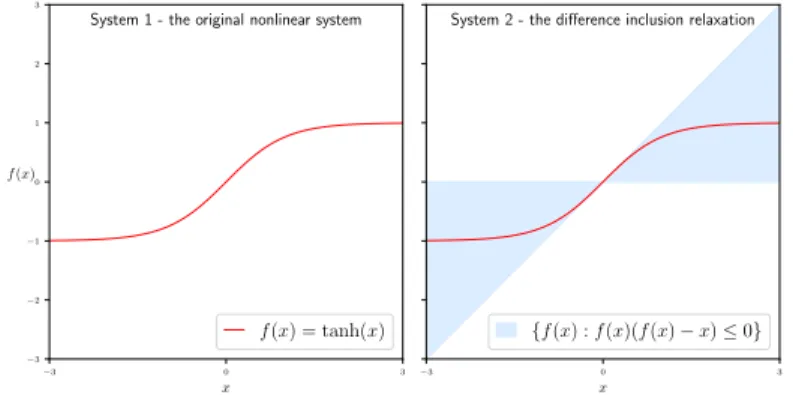
some chosen fixed quadratic constraints that those nonlinearities are known to satisfy, in order to simplify analysis. Figure 2-1 shows a contrived example to illustrate the

main idea. For both systems, the dynamics can be written as 𝑥+ _{= (𝑓 (𝑥) + 𝑥) /3: a}

linear term plus a state-dependent nonlinearity expressed as 𝑓(𝑥). The distinction is that in system I, 𝑓 = tanh(𝑥) plotted as the red line is a difference equation; whereas in system II, 𝑓(𝑥) is a difference inclusion that is allowed to take any possible value as long as it satisfies {(𝑓 (𝑥) − 𝑥) 𝑓(𝑥) ≤ 0}, which is plotted as the blue region. This difference inclusion is, in fact, very widely-used. It is due to Lur’e and is called the sector condition, and we will revisit it later.

Note that since any 𝑥 and 𝑓 = tanh(𝑥) pair respects the inequality (𝑓(𝑥) −

𝑥)𝑓 (𝑥)≤ 0 defining the sector set, the hyperbolic tangent nonlinearity belongs to the

sector. Visually, the blue region encompasses the red line. This containment means that any trajectory that system I could possibly produce is also a member in the

(27)

set of trajectories system II could produce. Now if system II is stable or ℓ2 stable

locally or globally, then any subset of those trajectories under consideration must

also be stable or ℓ2 stable, including the subset that corresponds to system I. By this

rationale, system II becomes a relaxation of system I in terms of stability/robustness analysis and serves as a surrogate for our analysis. We note that the full version with an integral involves a bit more reasoning but follows the same high level relaxation logic. −3 0 3 x −3 −2 −1 0 1 2 3 f (x)

System 1 - the original nonlinear system

f (x) = tanh(x)

−3 0 3

x

System 2 - the difference inclusion relaxation

{f(x) : f(x)(f(x) − x) ≤ 0}

Figure 2-1: IQC tutorial example. For both systems, the dynamics is 𝑥+ _{= (𝑥 +}

𝑓 (𝑥))/3where 𝑓(𝑥) is a difference equation for system I and a difference inclusion for

system II.

A natural question arises as to why would one take such a detour in analysis. The virtue lies in that the system II is easier to analyze. The constraints, now quadratic, are directly compatible with the aforementioned framework. Specifically, direct application of the Lyapunov condition Eq. (2.1) for global stability analysis and S-procedure Eq. (2.2) requires solving:

find 𝑃 > 0, 𝜆 > 0 s.t. 𝑃 𝑥2_{− 𝑃 (𝑥 + 𝑓)}2_/9 ⏟ ⏞ −Δ𝑉 + 𝜆(𝑓_⏟ _⏞− 𝑥)𝑓 S-procedure constraining 𝑥 and 𝑓 > 0 ∀𝑥, 𝑓 (2.4)

Simple algebra shows 𝑃 = 4, 𝜆 = 1 makes Eq. (2.4) feasible, meaning system II is stable. And by the relaxation logic, this implies that system I is stable.

Notice here the Lyapunov difference plays the role of −𝑇 and the sector condition

(28)

blue sector region, which is non-convex, could be encoded into a convex optimization problem. The process is indeed subtle: the non-convex constraint is on 𝑥 and 𝑓(𝑥), neither appears as decision variable in Eq. (2.4); instead, the decision variable is the multiplier 𝜆 whose only constraint, the sign condition, is convex. Peeling one layer deeper, note that the implication of Eq. (2.2) =⇒ Eq. (2.3) is true regardless of the

convexity of both 𝑇 and 𝑄𝑖 on 𝑥1.

1_{In fact, the implication is true for non-quadratic functions as well; the assumption of everything}

quadratic is again for computational reasons. Quadratic is believed to be the sweet spot between conservatism (rich enough a class of function) and computational cost; it also comes with the benefit of easily describable as an SDP [45].

(29)

Part I

Scalable Optimization-Based

Verification

(30)

(31)

Chapter 3 Compositional Verification

This chapter is adapted from work previously published in [65].

3.1 Introduction

As described in Section 2.1, LMIs are ubiquitous in system analysis, largely due to their clean connection to Lyapunov theory. It is widely known that most of the com-mon LTI systems analysis and synthesis tasks directly translate through Lyapunov argument into LMIs [13]. More recently, the development of sum-of-squares (SOS) programming makes it possible to essentially apply this technique in polynomial sys-tems as well [51], expanding the applicability even further.

Practically, however, LMIs and, by extension, SOS do not scale very well, and the computational cost is immense for large-scale systems. This computational challenge of SOS-based approaches for large-scale systems, combined with the natural decom-position structure arising from many such systems, motivates research areas such as compositional analysis [4, 78] and distributed and decentralized control [59, 6]. The common theme there is to not investigate the high-dimensional system directly. In-stead, the large system is first divided and studied in parts, and the implications of these individual results would then be reasoned about collectively for the original system.

(32)

typically materialized as the search of block-diagonal Lyapunov matrices. Various necessary and sufficient conditions on their existence have been given in the literature, but they are either restrictive or non-constructive. The restriction is usually on the dynamics matrix 𝐴 having a special structure such as being a Metzler matrix [48], block triangular, or cyclic [5], or on the Lyapunov matrix having particular block-diagonal patterns such as strictly block-diagonal [8, 67, 81, 72] or being limited to a 2-by-2 partition [69]. For the more general conditions, such as in [18], there is no simple recipe for computing the desired Lyapunov matrix from the sufficient rank conditions given. Our work offers sufficient constructive conditions without any of these structural limitations.

For compositional analysis of the more general polynomial systems via the SOS framework, we mention [78, 68, 3], which are most similar to ours. In previous work, the Lyapunov value constraints are untangled but their time derivatives are not; ours completely decouples both. We also note in particular that [3] focuses more on revealing a latent modular structure using graph partition ideas; we, on the other hand, assume the system has a given decomposition structure or one obvious enough by visual inspection and strive purely for efficiency. Our views are thus complementary, and combining them can solve a larger class of problems faster, as will be shown later by an example.

In Section 3.2, we formalize the problem and introduce technical background. In Section 3.3, we focus on finding block-diagonal Lyapunov matrix for LTI system, and present two algorithms for dynamics matrices of arbitrary size, structure, and parti-tion pattern. In Secparti-tion 3.4, we address the extension to polynomial dynamics and formulate a much smaller SOS programming. Finally, we demonstrate on numerical and practical examples in Section 3.5 the efficiency of the proposed algorithms.

Notation For a real vector 𝑥 ∈ R𝑛, the usual Euclidean 2-norm is denoted as

‖𝑥‖, the weighted 2-norm is denoted as ‖𝑥‖2

𝐴 := 𝑥′𝐴𝑥 with 𝐴 ∈ R𝑛×𝑛, and the time

derivatives are denoted as ˙𝑥. If 𝑥𝑖 ∈ R𝑛𝑖, 𝑖 = 1, 2, . . . , 𝑚, then (𝑥1, 𝑥2, . . . , 𝑥𝑚)denotes

their column catenation. For a matrix 𝐴 ∈ R𝑚×𝑛_{, 𝜎}

(33)

and 𝐴′ _{its transpose. 𝐴 ≻ 0 (resp. 𝐴 ⪰ 0) implies 𝐴 is square, symmetric, and}

positive definite (resp. positive semidefinite). If 𝐴𝑖 ∈ R𝑘𝑖×𝑘𝑖, 𝑖 = 1, 2, . . . , 𝑚, then

⨁︀𝑚

𝑖=1𝐴𝑖 := 𝐴1⊕ 𝐴2· · · ⊕ 𝐴𝑚 denotes the block diagonal matrix with diagonal blocks

𝐴1, 𝐴2, . . . , 𝐴𝑚. 𝐼 denotes the identity matrix of appropriate size. Symbol ∖ denotes

set complement. R[𝑥] denotes the ring of scalar polynomial functions in indeterminate

𝑥 with real coefficients, and R[𝑥]𝑚×𝑛 _{denotes an 𝑚 by 𝑛 matrix whose elements are}

scalar polynomials in R[𝑥].

3.2 Problem Statement

Consider a time-invariant polynomial system described by ˙𝑥 = 𝑓(𝑥) where the state

𝑥_{∈ R}𝑛 _{and the dynamics 𝑓 ∈ R[𝑥]}𝑛_{. We restrict ourselves to time-invariant systems}

and will drop all time dependencies. Let the state 𝑥 be partitioned into 𝑚 components: 𝑥 = (𝑥1, 𝑥2, . . . 𝑥𝑚), where 𝑥𝑖 ∈ R𝑛𝑖 constitutes the states of a subsystem. We assume

the partition is one such that no more than two subsystems are coupled, i.e., no terms like 𝑥11𝑥22𝑥32 (𝑥11 being the first state in the first subsystem and so on) exist in 𝑓.

This is not a restrictive assumption as it can always be satisfied by regrouping (e.g.,

one can merge 𝑥1 and 𝑥2 into a new sub-system should terms like 𝑥11𝑥22𝑥32 appear).

With the partition and assumption above, ˙𝑥 = 𝑓(𝑥) can be rearranged into a component-wise expanded form:

˙𝑥𝑖 = 𝑓𝑖(𝑥𝑖) + 𝑚 ∑︁ 𝑗=1 𝑗̸=𝑖 𝑔𝑖𝑗(𝑥𝑖)ℎ𝑖𝑗(𝑥𝑗) (3.1)

where 𝑓𝑖 ∈ R[𝑥𝑖]𝑛𝑖 describes the internal dynamics of sub-state 𝑥𝑖, 𝑔𝑖𝑗 ∈ R[𝑥𝑖]𝑛𝑖×𝑙𝑖𝑗𝑛𝑗

and ℎ𝑖𝑗 ∈ R[𝑥𝑗]𝑙𝑖𝑗𝑛𝑗 captures the coupling between sub-state 𝑥𝑖 and 𝑥𝑗. The newly

introduced dimension 𝑙𝑖𝑗 is due to the possibility of more than one linearly independent

coupling terms involving 𝑥𝑖 and 𝑥𝑗, for instance, say ˙𝑥1 =−𝑥13+ 𝑥1𝑥2+ 3𝑥12𝑥22, then

𝑙12 = 2. For the special LTI case, 𝑙𝑖𝑗 = 1, ∀𝑖, 𝑗.

We are interested in making claims such as asymptotic stability to the origin and invariance for the entire system states 𝑥, but ideally by examining one sub-system

(34)

state 𝑥𝑖 at a time. To this end, we associate the system with a Lyapunov-like function 𝑉 such that: 𝑉 (𝑥) = 𝑚 ∑︁ 𝑖=1 𝑉𝑖(𝑥𝑖)≥ 0, ∀𝑥 ∈ R𝑛 (3.2a) ˙ 𝑉 (𝑥) = 𝑚 ∑︁ 𝑖=1 ˙ 𝑉𝑖 < 0,∀𝑥 ∈ D (3.2b)

where the equality in Eq. (3.2a) holds only at the origin, and the region D in Eq. (3.2b) varies with the task in hand. For instance, when dealing with global stability

to the origin, D = R𝑛_{∖{0}, whereas in local analysis the region is usually a sub-level}

set of 𝑉 and part of the decision variables.

The aim in this section is to find the set of {𝑉𝑖}𝑚𝑖=1 functions independently so as

to form as small an LMI or SOS as possible. Eq. (3.2a) is already in a decoupled

form, and one can simply require 𝑉𝑖 ≥ 0, ∀𝑖. Eq. (3.2b) may look decoupled too, and

one may be tempted to claim that ˙𝑉𝑖 < 0,∀𝑖 is also a set of independent constraints;

this is not true. Note that ˙ 𝑉𝑖 = 𝜕𝑉𝑖(𝑥𝑖) 𝜕𝑥𝑖 𝑓𝑖+ 𝑚 ∑︁ 𝑗=1 𝑗̸=𝑖 𝜕𝑉𝑖(𝑥𝑖) 𝜕𝑥𝑖 𝑔𝑖𝑗(𝑥𝑖)ℎ𝑖𝑗(𝑥𝑗) (3.3)

while the first term is only dependent on 𝑥𝑖, the second term that is the summation

involves ℎ𝑖𝑗, a function of sub-states 𝑥𝑗, and the summing over all 𝑗 ̸= 𝑖 makes ˙𝑉𝑖

dependent on possibly the entire states 𝑥 = (𝑥1, 𝑥2, . . . 𝑥𝑚). This is a direct

conse-quence of sub-states coupling from the dynamics ˙𝑥𝑖, in other words, the set of { ˙𝑉𝑖}𝑚𝑖=1

are inherently entangled.

Our compositional approach thus avoids dealing with { ˙𝑉𝑖}𝑚𝑖=1 head-on. Instead,

we resort to finding an upper bound of ˙𝑉 that is by design a sum of functions each

dependent on one 𝑥𝑖 only. We then require this upper bound to be non-positive to

sufficiently imply Eq. (3.2b). While this detour leads to more conservative results, it allows the parallel search we desire and can bypass the computational hurdle of direct optimizations. The details of our approach are in Section 3.3 and 3.4.

(35)

3.3 LTI Systems and Block-Diagonal Lyapunov

Ma-trix

We first study the most fundamental LTI systems. Though the technical result in this section can be reduced from the polynomial systems’ result, some more intuitive aspects of it can only be or are better appreciated in this limited setting and hence it merits the separate elaboration here.

Under the LTI assumption, Eq. (3.1) takes a clean form ˙𝑥𝑖 = 𝐴𝑖𝑖𝑥𝑖+ 𝑚 ∑︁ 𝑗=1 𝑗̸=𝑖 𝐴𝑖𝑗𝑥𝑗 (3.4)

where 𝐴𝑖𝑖∈ R𝑛𝑖×𝑛𝑖, 𝐴𝑖𝑖𝑥𝑖 corresponds to the 𝑓𝑖 term, 𝐴𝑖𝑗 ∈ R𝑛𝑖×𝑛𝑗 corresponds to 𝑔𝑖𝑗

with dimension 𝑙𝑖𝑗 ≡ 1, and 𝑥𝑗 corresponds to the ℎ𝑖𝑗 term.

For LTI systems, it only makes sense to consider global asymptotic stability (to the origin) as all convergences in LTI systems are in the global sense. A quadratic

parameterization of Lyapunov function 𝑉 = 𝑥′_{𝑃 𝑥}_{such that 𝑃 ≻ 0 and 𝐴𝑃 + 𝑃 𝐴}′ _≺

0 is both necessary and sufficient for this task. Naturally then, when considering

Lyapunov functions for the subsystems, we use this quadratic parameterization as

well and let 𝑉𝑖 = 𝑥′𝑖𝑃𝑖𝑥𝑖. This is equivalent to imposing a block-diagonal structure

constraint on 𝑃 ≻ 0 as 𝑃 = ⨁︀𝑚

𝑖=1𝑃𝑖 ≻ 0. Substituting the parameterization into

condition Eq. (3.2) yields:

find {𝑃𝑖}𝑚𝑖=1 (3.5a) s.t. 𝑃𝑖 ≻ 0, ∀𝑖 (3.5b) ⎡ ⎢ ⎢ ⎢ ⎢ ⎢ ⎢ ⎣ 𝐴11𝑃1+ 𝑃1𝐴′11 . . . 𝐴1𝑛𝑃𝑛+ 𝑃1𝐴′𝑛1 𝐴21𝑃1+ 𝑃2𝐴′12 . . . 𝐴2𝑛𝑃𝑛+ 𝑃2𝐴′𝑛2 ... ... ... 𝐴𝑛1𝑃1+ 𝑃𝑛𝐴′1𝑛 . . . 𝐴𝑛𝑛𝑃𝑛+ 𝑃𝑛𝐴′𝑛𝑛 ⎤ ⎥ ⎥ ⎥ ⎥ ⎥ ⎥ ⎦ ≺ 0, (3.5c)

(36)

𝐸𝑞. (3.2b). The clean block-diagonal structure in 𝑃 is deeply buried here as the left hand side is a full matrix with 𝐴𝑖𝑗𝑃𝑗+ 𝑃𝑖𝐴′𝑗𝑖 at all the off-diagonal spots.

Our goal in this section is to find the set of {𝑃𝑖}𝑚𝑖=1 independently for each 𝑖. We

start with an LMI-based algorithm that is still somewhat coupled, and then gradually get to the truly decoupled algorithm which is based on Riccati equations.

3.3.1 Sparse LMIs

Theorem 1. For an 𝑛-dimensional LTI system written in the form Eq. (3.4), if the

optimization problem find _{𝑃𝑖}𝑚𝑖=1,{𝑀𝑖𝑗}𝑚𝑖,𝑗=1,𝑖̸=𝑗 (3.6a) s.t. 𝑃𝑖 ≻ 0, ∀𝑖 (3.6b) 𝑀𝑖𝑗 ≻ 0, ∀𝑖, 𝑗, 𝑖 ̸= 𝑗 (3.6c) 𝐴𝑖𝑖𝑃𝑖+ 𝑃𝑖𝐴′𝑖𝑖+ 𝑚 ∑︁ 𝑗=1 𝑗̸=𝑖 𝐴𝑖𝑗𝑀𝑖𝑗𝐴′𝑖𝑗 + 𝑃𝑖𝑀𝑗𝑖−1𝑃𝑖 ≺ 0, ∀𝑖 (3.6d)

is feasible, then the set of _{𝑃𝑖}𝑚𝑖=1 satisfies problem Eq. (3.5) with D = R𝑛∖{0}, and

the original system is strictly asymptotically stable.

Proof. Two proofs, one from the primal perspective and the other the dual, are

in-cluded in the chapter appendix. Theorem 1 can also be reduced from Theorem 2 (in Subsection 3.4), whose proof is in fact less involved. The appended proofs, however, offer a control and optimization connection that the simple proof lacks.

Remark 1. Theorem 1 can be viewed as a generalization of the sufficient direction of Lyapunov inequality for LTI systems. Particularly, if the state is not partitioned,

𝑃 has no structural constraint, the summation in Eq. (3.6d) disappears, and the

condition reduces to the ordinary Lyapunov inequality. Furthermore, Theorem 1 gives an explicit procedure to construct a Lyapunov matrix with user specified structures including the extreme case of pure diagonal structure.

(37)

Remark 2. Theorem 1 also closely resembles the small-gain theorem (which in fact is

the inspiration for our results). Notice that setting 𝑚 = 2 (two subsystems scenario)

reduces Theorem 1 to the matrix version of the bounded real lemma, which proves

the product of the two subsystems’ ℓ2-gains less than or equal to one and implies

stability. The intuition behind the connection is this: think of diagonal blocks𝐴11 and

𝐴22 as describing two disconnected “nominal” plants, and the off-diagonal blocks are

pumping feedback disturbance from one nominal system to the other. The compound system admitting a block-diagonal Lyapunov matrix indicates it is stable whether or not the disturbance blocks are present, and this is exactly what small-gain theorem implies. The feedback disturbance interpretation obviously carries over to more than two interconnected systems even though there is no extension of small-gain theorem

in those settings. (The structured disturbance setup arising from 𝜇-synthesis is not

such a generalization. While it does admit multi-dimensional disturbances, all the disturbances are to the central nominal plant but not to one another.) We illustrate the system assumptions difference between the two versions of small-gain and ours in Figure 3-1.

Remark 3. One might wonder what is the virtue of studying the bare bone Lyapunov inequality; after all, checking stability can easily be done through an eigenvalue com-putation and that is uniformly faster than LMIs. We believe the value lies in that LMIs is more general and clean than eigen-based methods. For instance, LMI for-mulation leads to extensions such as robustness analysis via common Lyapunov func-tions which eigen-based method fails to handle; or to a straightforward formulation

of ℓ2-gain bound, for which the eigen-based method leads to very messy computation.

Therefore, 𝐴𝑃 + 𝑃 𝐴′_{, the most basic building block appearing in almost every control}

LMI, deserves a close examination.

Remark 4. Computationally, Eq. (3.6d) with the nonlinear term 𝑃𝑖𝑀𝑗𝑖−1𝑃𝑖 can be

equivalently turned into an LMI via Schur complement. Hence, Theorem 1 requires

solving 𝑚 coupled LMIs of the original problem size, but all of them enjoy strong

(38)

cor-Figure 3-1: Our setup compared with the unstructured and structured small-gain setup. Our setup takes advantage of the ‘weak’ internal interconnection, thus achieve a ‘balance’ between the unstructured and structured cases.

responding column, and the main diagonal. For instance, when 𝑚 = 8, Figure 3-2

shows the sparsity pattern of three out of the eight LMIs. The sparsity in practice might already be a worthy trade off, and we test the claim in Section 3.5. Further,

if we fix the set of 𝑀𝑖𝑗 rather than searching for them, constraints Eq. (3.6) become

decoupled low-dimensional LMIs. Better yet, they can be solved by an even faster Riccati equation based method below.

(39)

3.3.2 Riccati Equations

If 𝑀𝑖𝑗 are fixed, the set of decoupled low-dimensional LMIs can be solved by a method

based on Riccati equations, which has near-analytical solutions and by implication far better scalability and numerical stability than LMIs. Specifically, if we replace the inequality with equality, then Eq. (3.6) are precisely Riccati equations with

un-known 𝑃𝑖. The feasibility of LMIs like Eq. (3.6) is equivalent to the feasibility of

the associated Riccati equations. That is, the (unique) positive definite solution to the Riccati equation lives on the boundary of the feasible set of the LMI [13]. So by nudging the right hand side in the constraint slightly in the positive direction, e.g., replacing zero with 𝜖𝐼 for some small 𝜖 > 0, we get a solution strictly in the interior and one precise to the original LMI. We note that when the Riccati equations return a feasible solution, it is much faster than solving the sparse LMIs Eq. (3.6), and even more significantly so than the original LMI Eq. (3.5).

The choice of the set of positive definite 𝑀𝑖𝑗 scaling matrices can be arbitrary but

would largely affect the feasibility. Identity scaling is one obviously valid choice, and it is very likely to succeed in cases such as when the off-diagonal blocks are very close to zeros. In general though, identity scaling is not guaranteed to always work, it is then desirable to have some other heuristics at our disposal. Inspired by the small-gain theorem connection in Remark 2, we propose another educated guess that we call 𝜎1-scaling. The procedure is to first initialize a set of scalars 𝛾𝑖𝑗 = 𝜎1(𝐴𝑖𝑖−1𝐴𝑖𝑗); then

keep 𝛾𝑖𝑗 as is if 𝛾𝑖𝑗𝛾𝑗𝑖 ≤ 1, otherwise, say 𝛾𝑖𝑗 > 𝛾𝑗𝑖−1, then keep only 𝛾𝑗𝑖 and shrink 𝛾𝑖𝑗

down to 𝛾−1

𝑗𝑖 ; and finally set 𝑀𝑖𝑗 = 𝛾𝑖𝑗𝐼. The justification of the heuristic is that 𝜎1

operator of a dynamics matrix loosely reflects the input-output signal magnification

by the system, and 𝜎1(𝐴𝑖𝑖−1𝐴𝑖𝑗) can therefore serve as a barometer of the relative

energy exchange between an internal 𝐴𝑖𝑖 subsystem and the coupling 𝐴𝑖𝑗 term from

system 𝑗. Of course, there is no guarantee on the performance of 𝜎1-scaling either.

Empirically though, they succeed roughly 7 times out of 10. Plus, the time it takes to test these scalings is negligible compared with solving any LMIs, so it is well worth a try.

(40)

3.4 Polynomial Systems and Compositional SOS

Lya-punov Functions

Extending the LTI decoupling idea to polynomial systems is conceptually straightfor-ward: we again want to upper bound ˙𝑉 . Technically, a few nice properties from the LTI case would vanish. We will discuss these issues when they appear, and for now start with the result for global asymptotic stability (g.a.s.).

Theorem 2. For a polynomial system described in the expanded form Eq. (3.1), if

find _{𝑉𝑖}𝑚_𝑖=1,{𝑀𝑖𝑗}𝑚_{𝑖,𝑗=1,𝑖̸=𝑗} (3.7a) s.t. 𝑀𝑖𝑗 ≻ 0, ∀𝑖, 𝑗, 𝑖 ̸= 𝑗 (3.7b) 𝑉𝑖− 𝜖‖𝑥𝑖‖ is SOS, ∀𝑖 (3.7c) − 𝜕𝑉𝑖 𝜕𝑥𝑖 𝑓𝑖− 1 2 𝑚 ∑︁ 𝑗=1 𝑗̸=𝑖 ‖𝜕𝑉𝑖 𝜕𝑥𝑖 𝑔𝑖𝑗‖2𝑀𝑖𝑗 − 1 2 𝑚 ∑︁ 𝑗=1 𝑗̸=𝑖 ‖ℎ𝑗𝑖‖2_𝑀−1 𝑗𝑖 − 𝜖‖𝑥𝑖‖ is SOS, ∀𝑖 (3.7d)

is feasible for some 𝜖 > 0, then the set of polynomial functions {𝑉𝑖(𝑥𝑖)}𝑚_𝑖=1 satisfies

Eq. (3.2) with D = R𝑛_{∖{0} and the system is (g.a.s.) at the origin.}

Proof. Eq. (3.7c) obviously implies Eq. (3.2a). Then introducing invertible matrices

𝑚𝑖𝑗 ∈ R𝑙𝑖𝑗𝑛𝑗×𝑙𝑖𝑗𝑛𝑗 and let 𝑀𝑖𝑗 = 𝑚𝑖𝑗𝑚′𝑖𝑗, we can have ˙𝑉 upper bounded:

˙ 𝑉 = 𝑚 ∑︁ 𝑖=1 ⎛ ⎜ ⎜ ⎝ 𝜕𝑉𝑖 𝜕𝑥𝑖 𝑓𝑖+ 𝑚 ∑︁ 𝑗=1 𝑗̸=𝑖 𝜕𝑉𝑖 𝜕𝑥𝑖 𝑔𝑖𝑗ℎ𝑖𝑗 ⎞ ⎟ ⎟ ⎠ (3.8a) = 𝑚 ∑︁ 𝑖=1 𝜕𝑉𝑖 𝜕𝑥𝑖 𝑓𝑖+ 𝑚 ∑︁ 𝑖=1 𝑚 ∑︁ 𝑗=1 𝑗̸=𝑖 (︂ 𝜕𝑉𝑖 𝜕𝑥𝑖 𝑔𝑖𝑗𝑚𝑖𝑗𝑚−1𝑖𝑗 ℎ𝑖𝑗 )︂ (3.8b) ≤ 𝑚 ∑︁ 𝑖=1 𝜕𝑉𝑖 𝜕𝑥𝑖 𝑓𝑖+ 1 2 𝑚 ∑︁ 𝑖=1 𝑚 ∑︁ 𝑗=1 𝑗̸=𝑖 (︂ ‖𝑔𝑖𝑗 𝜕𝑉𝑖 𝜕𝑥𝑖‖ 2 𝑀𝑖𝑗 +‖ℎ𝑖𝑗‖ 2 𝑀_𝑖𝑗−1 )︂ (3.8c) = 𝑚 ∑︁ 𝑖=1 ⎛ ⎜ ⎜ ⎝ 𝜕𝑉𝑖 𝜕𝑥𝑖 𝑓𝑖+ 1 2 𝑚 ∑︁ 𝑗=1 𝑗̸=𝑖 (︂ ‖𝜕𝑉_𝜕𝑥𝑖 𝑖 𝑔𝑖𝑗‖2𝑀𝑖𝑗 +‖ℎ𝑗𝑖‖ 2 𝑀_𝑗𝑖−1 )︂⎞_⎟ ⎟ ⎠ (3.8d)

(41)

Eq. (3.8c) is due to the elementary inequality of arithmetic and geometric means (AM-GM inequality), and the exchange of summation index at Eq. (3.8d) is due to the symmetry between 𝑖 and 𝑗. Eq. (3.7d) implies the negation of Eq. (3.8d) is SOS, which directly leads to that the negation of ˙𝑉 is SOS, and sufficient to imply Eq. (3.2b).

Remark 5. Our method can be extended to handle coupling terms such as 𝑥𝑖𝑥𝑗𝑥𝑘

that involves more than two sub-states. The key step is to use the generalized version

of AM-GM inequality with 𝑛 > 2 variables at Eq. (3.8c).

Remark 6. Similar to the LTI case, the scaling matrices 𝑀𝑖𝑗 brings coupling across

the constraints. Eliminating these constants as decision variables could again untangle

the entire set of constraints. However, we do not believe a trivial extension of 𝜎1

-scaling developed for the LTI case would be as convincing a heuristic for hand-picking these constants in the polynomial settings. This is mainly due to the lack of a notion of ‘coupling strength’ in the polynomial sense. Specifically, for LTI systems, the coupling can only enter as 𝐴𝑖𝑗𝑥𝑖𝑥𝑗, so at least intuitively, for a ‘normalized’ 𝐴𝑖𝑖 the strength

of the coupling is quantified by 𝐴𝑖𝑗. Polynomial systems with the additional freedom

of degrees, however, can have coupling terms like 4𝑥𝑖𝑥𝑗 and 𝑥𝑖𝑥2𝑗. It is then hard

to argue, even hand-wavingly, if the coefficients play a more important role or if the

degrees do. Therefore, we settle with just fixing all the 𝑀𝑖𝑗 to identity.

Remark 7. Even with 𝑀𝑖𝑗 = 𝐼, the term ‖𝜕𝑉_𝜕𝑥𝑖

𝑖𝑔𝑖𝑗‖

2 _{in Eq.} _{(3.7d) is still not directly}

valid for a SOS program because of the quadratic dependency on 𝑉𝑖. We develop below

what can be considered the generalization of Schur complement in the polynomial settings to legalize the constraint.

Lemma 1. Given a scalar SOS polynomial 𝑞(𝑥) _{∈ R[𝑥] of degree 2𝑑}𝑞 and a vector

of generic polynomials 𝑠(𝑥) ∈ R[𝑥]𝑛 _{of maximum degree} _𝑑

𝑠, let 𝑦 be a vector of

indeterminates whose elements are independent of 𝑥, then 𝑞(𝑥)_{− 𝑠}′_{(𝑥)𝑠(𝑥)}_{∈ R[𝑥] is}

SOS if and only if 𝑞(𝑥) + 2𝑦′𝑠(𝑥) + 𝑦′𝑦 ∈ R[𝑥, 𝑦] is SOS.

Proof. Define 𝑚 (𝑥) and 𝑛(𝑥, 𝑦) respectively as the standard monomial basis of 𝑥

(42)

𝐶′_𝑚(𝑥) _{for some coefficients 𝐶, and 𝑞(𝑥) = 𝑚}′_{(𝑥) [𝑄 + 𝐿 (𝛼}

1)] 𝑚(𝑥), where Q is

a constant symmetric matrix such that 𝑞(𝑥) = 𝑚′_{(𝑥)𝑄𝑚(𝑥), 𝐿(𝛼}

1) is a

param-eterization of the linear subspace ℒ := {𝐿 = 𝐿′ _{: 𝑚}′_{(𝑥)𝐿(𝛼)𝑚(𝑥) = 0}_{}, and}

𝑄 + 𝐿(𝛼1) ⪰ 0. Denote 𝑞(𝑥) − 𝑠′(𝑥)𝑠(𝑥) as Π1 and plug in these parameterizations,

Π1 = 𝑚′(𝑥) [𝑄 + 𝐿(𝛼1)− 𝐶′𝐶] 𝑚(𝑥).

If Π1 is SOS, then there exists an 𝐿(𝛼2) ∈ ℒ (possibly different from 𝐿(𝛼1))

such that 𝑄 + 𝐿(𝛼1)− 𝐶′𝐶 + 𝐿(𝛼2) ⪰ 0. This implies via Schur complement that

𝑉 := [︀𝑄+𝐿(𝛼1)+𝐿(𝛼2) 𝐶′

𝐶 𝐼

]︀

⪰ 0. Denote 𝑞(𝑥) + 2𝑦′_{𝑠(𝑥) + 𝑦}′_𝑦 _{as Π}

2 and notice that it is

precisely (𝑚(𝑥), 𝑦)′_{𝑉 (𝑚(𝑥), 𝑦), and therefore Π}

2 is SOS.

If Π2 is SOS, then there exists a 𝛽1 such that Π2 = 𝑛′(𝑥, 𝑦) [𝑇 + 𝑀 (𝛽1)] 𝑛(𝑥, 𝑦)

where 𝑇 is a constant symmetric matrix such that 𝑛′_{(𝑥, 𝑦)𝑇 𝑛(𝑥, 𝑦) = Π}

2, 𝑀(𝛽1) is a

parameterization of the linear subspace ℳ := {𝑀 = 𝑀′ _{: 𝑛}′_{(𝑥, 𝑦)𝑀 (𝛽)𝑛(𝑥, 𝑦) =}

0}, and 𝑇 + 𝑀(𝛽1) ⪰ 0. Since the elements of 𝑚(𝑥) and 𝑦 form a strict

sub-set of those in 𝑛(𝑥, 𝑦), the ordering 𝑛(𝑥, 𝑦) = (𝑚(𝑥), 𝑦, 𝑘(𝑥, 𝑦)) where 𝑘

encapsu-lates the 𝑥, 𝑦 cross term monomials is possible. Accordingly, 𝑇 + 𝑀(𝛽1) can be

partitioned as [︁𝑇11+𝑀11𝑇12+𝑀12 𝑇13+𝑀13

* 𝑇22+𝑀22 𝑇23+𝑀23

* * 𝑇33+𝑀33

]︁

(𝛽1 from now on dropped for concision).

Then, since Π2 has no cross terms of second or higher order in 𝑦, it must be that

𝑘′_{(𝑥, 𝑦) [𝑇}

33+ 𝑀33] 𝑘′(𝑥, 𝑦) = 0, and since 𝑦 and 𝑥 are independent, 𝑇33+ 𝑀33 = 0.

Similar arguments imply that 𝑇23+ 𝑀23 = 𝑇32′ + 𝑀32′ = 0, and 𝑇22+ 𝑀22= 𝐼. Once

these four blocks are fixed, by the equality constraint in the Schur complement of 𝑇11+

𝑀11, it must be the case that 𝑇13+𝑀13 = 𝑇31′ +𝑀31′ = 0. In other words, Π2 in fact

ad-mits a more compact expansion Π2 = (𝑚 (𝑥) , 𝑦)′

[︀_𝑇₁₁_+𝑀₁₁ _𝑇₁₂_+𝑀₁₂

* 𝐼

]︀

(𝑚 (𝑥) , 𝑦)where by

matching the terms and invoking the independence of 𝑥 and 𝑦, 𝑚′_{(𝑥) [𝑇}

11+ 𝑀11] 𝑚(𝑥) =

𝑞(𝑥), 𝑚′_{(𝑥) [𝑇}

12+ 𝑀12] = 𝑠(𝑥), and the gram matrix is positive semi-definite. The

Schur complement of the 𝐼 block therefore gives an explicit SOS parameterization of

Π1 in 𝑚(𝑥).

Lemma 1 trivially extends to “𝑞(𝑥)₋∑︀𝑚_𝑗=1_‖𝑠𝑗(𝑥)‖2 is SOS”, again via Schur

com-plement of the Gram matrix. The extended condition can be mapped to Eq. (3.7d),

with₋𝜕𝑉𝑖 𝜕𝑥𝑖𝑓𝑖− 1 2 ∑︀𝑚 𝑗=1 𝑗̸=𝑖‖ℎ𝑗𝑖‖ 2 _as_{𝑞(𝑥), and} 𝜕𝑉𝑖𝑔𝑖𝑗 √

2𝜕𝑥𝑖 as𝑠𝑗(𝑥). Now the constraint Eq.(3.7d)

(43)

3.5 Experiments and Examples

The examples are run on a MacBook Pro with 2.9GHz i7 processor and 16GB memory. The LMI problem specifications are parsed via CVX [25], SOS problems are parsed via SPOTLESS [76], and both are then solved via MOSEK [47]. The source code is available online.1

Randomly Generated LTI Systems We randomly generate 1000 candidate 𝐴

matrices of various sizes that admit block-diagonal Lyapunov matrices of various block sizes. We facilitate the sampling process by biasing 𝐴 towards negative block-diagonal dominance (to make it more likely an eligible candidate), and then pass this sample 𝐴 into the full LMI Eq. (3.5) to check if the LMI (a necessary and sufficient condition) produces a block-diagonal Lyapunov matrix, if not, the sample is rejected. Table 3.1 records the average run time comparison of this full LMI Eq. (3.5) and our proposed sparse LMIs Eq. (3.6) and Riccati equations algorithms. It also records the

success rate of identity scaling and 𝜎1-scalings for hand-picking the 𝑀𝑖𝑗 term in the

Riccati equations.

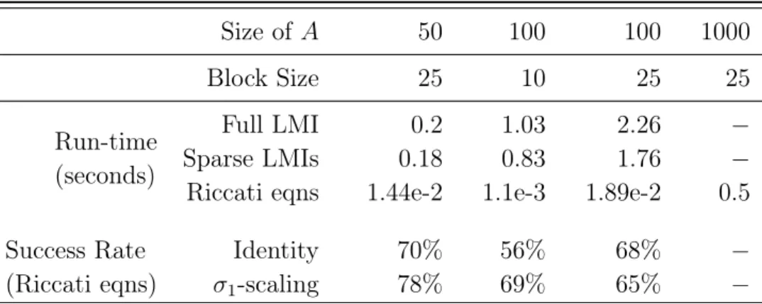
Table 3.1: Run-time and success rates for LTI systems

Size of 𝐴 50 100 100 1000 Block Size 25 10 25 25 Run-time (seconds) Full LMI 0.2 1.03 2.26 − Sparse LMIs 0.18 0.83 1.76 −

Riccati eqns 1.44e-2 1.1e-3 1.89e-2 0.5

Success Rate

(Riccati eqns) 𝜎1Identity-scaling 70%78% 56%69% 68%65% −−

The first two “−”s in the last column indicate the LMI-based methods run into memory issues and the solver is forced to stop. Riccati equations are still able to solve some of these sampled problems, but without the baseline LMI feasibility, its success rate is not available either, hence the last two “−”s. We note that when the

(44)

Riccati equations are feasible, they are the fastest method to check stability of the generated 𝐴 matrices. The computational saving becomes more significant as the dimension goes up thanks to scalable algorithms solving Riccati equations. We also

note that there is no clear winner between identity scaling and 𝜎1 scaling when it

comes to producing feasible Riccati equations. In practice, one may want to try both as there is very little added real time computational cost of doing so.

Lotka-Volterra System We take from [3] the Lotka-Volterra example and verify

its stability. It is a 16-dimensional polynomial system2, and is thus beyond the reach

of direct SOS optimization. In that paper, the authors handle the task by first developing a graph partition based algorithm, which finds a 3-way partition scheme for this example, and then a non-sparse or sparse SOS programs for computing a Lyapunov function for each subsystem and a composite Lyapunov function for the original system.

Their graph partition algorithm is of particular interest to us, since our composi-tional algorithm requires a partition but lacks the ability to search for one. Reusing their resulting 3-way partition scheme, we are also able to find a composite Lya-punov function. However, our underlying SOS formulations and hence run-time are significantly different.

Table 3.2: Run-time comparison for Lotka-Volterra system

Non-sparse alg.[3] Sparse alg. [3] Proposed

𝑉1 0.25s 0.38s 0.1023s

𝑉2 0.25s 0.37s 0.0587s

𝑉3 0.44s 0.59s 0.0568s

𝑉 1415.23s 688.54s 0.2178s

For both non-sparse and sparse algorithms in [3], after the individual {𝑉𝑖}3𝑖=1 are

found by low-dimensional SOS, it relies on an additional search of 𝛼𝑖 > 0 such that

∑︀

𝑖𝛼𝑖𝑉𝑖 satisfies the derivative condition in 𝑥. This has to be done with yet another

2_{we omit explicitly listing here the dynamics for saving space and refer the reader to the source}

(45)

SOS program of considerable size since the indeterminate is the high dimensional 𝑥.

Also, there is no guarantee such an 𝛼𝑖 > 0 always exists; it heavily depends on how

compatible {𝑉𝑖}3𝑖=1 are (in our test, the {𝑉𝑖}3𝑖=1 we found do not produce feasible 𝛼𝑖,

so we copy the run-time reported in the paper for comparison).

Our sufficient condition Eq. (3.7), in contrast, guarantees that ∑︀𝑖𝑉𝑖 would

auto-matically satisfy the derivative condition. This is done by imposing more restrictive

conditions on {𝑉𝑖}3𝑖=1 at the their independent construction stages. In other words,

once we get these ingredients, no extra work is necessary and the time spent

search-ing for 𝑉 is just the sum of time spent on each {𝑉𝑖}3𝑖=1 in much lower dimensions.

Consequentially, as shown in Table 3.2, our final run-time is 3-4 orders of magnitude faster in finding the composite 𝑉 .

This example showcases the combined power of graph partition-like algorithms such as [3] and the technique proposed in this paper: the former as a prepossessing step can extend the use case, and the latter can facilitate a much faster optimization program.

3.6 Discussion and Future Work

In this paper, general and constructive compositional algorithms are proposed for the computationally prohibitive problem of stability and invariance verification of large-scale polynomial systems. The key idea is to break the large system into several sub-systems, construct independently for each subsystem a Lyapunov-like function, and guarantee that their sum automatically certifies the original high-dimensional system is stable or invariant. The proposed algorithms can handle problems beyond the reach of direct optimizations, and are orders of magnitude faster than existing compositional methods.

We are interested in exploring extensions of our work to compositional safety verification of multi-agent networks by leveraging the barrier certificate idea [56]. We believe the connection is immediate both technically, as barrier certificates are natural extensions of Lyapunov function, and practically, as the multi-agent network has, by

(46)

definition, a compositional structure.

Appendix

Primal Proof of Theorem 1

Proof. Let us denote the left hand side of Eq. (3.5c) as 𝑈. Let 𝑈𝑘 be the k-th leading

principal sub-matrix of 𝑈 in the blocks sense (e.g., 𝑈1 equals 𝐴11𝑃1+ 𝑃1𝐴′11 instead

of the first scalar element in 𝑈), and let ˜𝑈𝑘 be the last column-blocks of 𝑈𝑘 with its

last block element deleted, i.e.,

˜ 𝑈𝑘 := ⎡ ⎢ ⎢ ⎢ ⎢ ⎢ ⎢ ⎣ 𝐴1𝑘𝑃𝑘+ 𝑃1𝐴′𝑘1 𝐴2𝑘𝑃𝑘+ 𝑃2𝐴′𝑘2 ... 𝐴_{(𝑘−1)𝑘}𝑃𝑘+ 𝑃𝑘−1𝐴′𝑘(𝑘−1) ⎤ ⎥ ⎥ ⎥ ⎥ ⎥ ⎥ ⎦

Also, define a sequence of matrices:

𝑁𝑘:= 𝑘 ⨁︁ 𝑖=1 (︃ _𝑚 ∑︁ 𝑗=𝑘+1 𝐴𝑖𝑗𝑀𝑖𝑗𝐴′𝑖𝑗 + 𝑃𝑖𝑀𝑗𝑖−1𝑃𝑖′ )︃

for 𝑘 = 1, 2, . . . , 𝑚 − 1, and 𝑁𝑘 = 0 for 𝑘 = 𝑚. Let ¯𝑁𝑘 be the largest principal minor

of 𝑁𝑘 in the block sense. It’s obvious then that by construction 𝑁𝑘⪰ 0, ∀𝑘.

We will use induction to show that 𝑈𝑘+ 𝑁𝑘 ≺ 0, ∀𝑘, so that in the terminal case

𝑘 = 𝑛, we would arrive at the desired Lyapunov inequality 𝑈 = 𝑈𝑛+ 𝑁𝑛 ≺ 0. For

𝑘 = 1, 𝑈1 + 𝑁1 ≺ 0 is trivially guaranteed by taking 𝑖 = 1 in Eq. (3.6d). Suppose

𝑈𝑘+ 𝑁𝑘 ≺ 0 for a particular 𝑘 ≤ 𝑛 − 1, let us now show that 𝑈𝑘+1+ 𝑁𝑘+1 ≺ 0.

First, notice that for 𝑘 ≤ 𝑛 − 1, the sequence of 𝑁𝑘 satisfies this recursive update:

𝑁𝑘 = 𝑛𝑘+ ¯𝑁𝑘+1 where 𝑛𝑘:= 𝑘 ⨁︁ 𝑖=1 (︁ 𝐴𝑖(𝑘+1)𝑀𝑖(𝑘+1)𝐴′𝑖(𝑘+1)+ 𝑃𝑖𝑀_(𝑘+1)𝑖−1 𝑃𝑖′ )︁

(47)

Notice also that 𝑛𝑘= 𝐿𝑘𝑆𝑘+1𝐿′𝑘 where 𝐿𝑘 :=[︁⨁︀𝑘_𝑖=1𝑃𝑖 , ⨁︀𝑘 𝑖=1𝐴𝑖(𝑘+1) ]︁ 𝑆𝑘+1 :=[︁⨁︀𝑘_𝑖=1𝑀_(𝑘+1)𝑖−1 ⊕⨁︀𝑘_𝑖=1𝑀𝑖(𝑘+1) ]︁

From the assumption that 𝑈𝑘+𝑁𝑘≺ 0, we have 𝑈𝑘+𝑁𝑘 = 𝑈𝑘+𝐿𝑘𝑆𝑘+1𝐿′𝑘+ ¯𝑁𝑘+1 ≺ 0.

Rearrange the terms:

− (𝑈𝑘+ ¯𝑁𝑘+1)≻ 𝐿𝑘𝑆𝑘+1𝐿′𝑘 (3.9)

Next, let 𝐷𝑘+1 be the left hand side of constraint Eq. (3.6d) at 𝑖 = 𝑘 + 1 with the

summation truncated to be only over indicies 𝑘 + 2 to 𝑛 (as opposed to be over all indices other than 𝑘 + 1), i.e.,

𝐷𝑘+1 :=𝐴(𝑘+1)(𝑘+1)𝑃𝑘+1+ 𝑃𝑘+1𝐴′(𝑘+1)(𝑘+1) + 𝑚 ∑︁ 𝑗=𝑘+2 𝐴(𝑘+1)𝑗𝑀(𝑘+1)𝑗𝐴′(𝑘+1)𝑗 + 𝑚 ∑︁ 𝑗=𝑘+2 𝑃𝑘+1𝑀(𝑘+1)𝑗𝑃𝑘+1 and let 𝑇𝑘+1 :=[𝐴(𝑘+1)1, 𝐴(𝑘+1)2, . . . , 𝐴(𝑘+1)𝑘, 𝑃𝑘+1, . . . , 𝑃𝑘+1 ⏟ ⏞ repeat k times ]

Then by Schur complement, constraint Eq. (3.6d) with 𝑖 = 𝑘 + 1 is equivalent to: ⎡ ⎢ ⎢ ⎢ ⎣ 𝐷𝑘+1 𝑇𝑘+1 𝑇′ 𝑘+1 −𝑆𝑘+1 ⎤ ⎥ ⎥ ⎥ ⎦≺ 0 (3.10)

Use Schur complement on Eq. (3.10) again, this time from the opposite direction, it is also equivalent to:

Convex optimization and machine learning for scalable verification and control

Convex Optimization and Machine Learning for

Scalable Verification and Control

by

Shen Shen

Submitted to the Department of Electrical Engineering and Computer

Science

in partial fulfillment of the requirements for the degree of

Doctor of Philosophy

at the

MASSACHUSETTS INSTITUTE OF TECHNOLOGY

September 2020

© Massachusetts Institute of Technology 2020. All rights reserved.

Author . . . .

Department of Electrical Engineering and Computer Science

July 31, 2020

Certified by. . . .

Russ Tedrake

Professor of Electrical Engineering and Computer Science

Thesis Supervisor

Accepted by . . . .

Leslie A. Kolodziejski

Professor of Electrical Engineering and Computer Science

Chair, Department Committee on Graduate Students

Convex Optimization and Machine Learning for Scalable

Verification and Control

by

Shen Shen

Abstract

Acknowledgments

Contents

I

Scalable Optimization-Based Verification

29

II

Verification of Neural Networks Systems

74

III

SafetyNet: Structured Learning and Optimization Knit

Together

102

List of Figures

List of Tables

Chapter 1

Introduction

1.1

Contribution

Chapter 2

Background

2.1

Lyapunov Functions and Linear Matrix

Inequal-ities

2.2

Sum-of-Squares (SOS) Programming

2.3

Integral Quadratic Constraints (IQC)

Part I

Scalable Optimization-Based

Verification

Chapter 3

Compositional Verification

3.1

Introduction

3.2

Problem Statement

3.3

LTI Systems and Block-Diagonal Lyapunov

Ma-trix

3.3.1

Sparse LMIs

3.3.2

Riccati Equations

3.4

Polynomial Systems and Compositional SOS

Lya-punov Functions

3.5

Experiments and Examples

3.6

Discussion and Future Work

Appendix