HAL Id: hal-01467738
https://hal.archives-ouvertes.fr/hal-01467738
Submitted on 2 May 2019
HAL is a multi-disciplinary open access
archive for the deposit and dissemination of
sci-entific research documents, whether they are
pub-lished or not. The documents may come from
teaching and research institutions in France or
abroad, or from public or private research centers.
L’archive ouverte pluridisciplinaire HAL, est
destinée au dépôt et à la diffusion de documents
scientifiques de niveau recherche, publiés ou non,
émanant des établissements d’enseignement et de
recherche français ou étrangers, des laboratoires
publics ou privés.
To cite this version:
W. Marzocchi, L. Sandri, Arnauld Heuret, F. Funiciello.
Where giant earthquakes may come.
Journal of Geophysical Research, American Geophysical Union, 2016, 121 (10), pp.7322-7336.
�10.1002/2016JB013054�. �hal-01467738�
Where giant earthquakes may come
W. Marzocchi1, L. Sandri2, A. Heuret3,4, and F. Funiciello3
1INGV, Rome, Italy,2INGV, Bologna, Italy,3Scienze Geologiche, Università Roma Tre, Rome, Italy,4Géosciences Montpellier,
Université de Guyane, France
Abstract
Giant earthquakes (Mw≥ 8.5) usually occur on the boundary between subducting and overriding plates of converging margins, but it is not yet clear which (if any) subduction zones are more prone to produce such a kind of events. Here we show that subduction zones may have different capabilities to produce giant earthquakes. We analyze the frequency-magnitude distribution of the interplateearthquakes at subduction zones that occurred during 1976–2007 and calculate the propensity (defined as the average annual rate) of giant events for about half of the subduction zones. We find that the b value of interplate earthquakes is significantly different among the subduction zones, and out-of-sample giant earthquakes (before 1976 and after 2007) have occurred preferentially in high-propensity areas. Besides the importance for seismic hazard assessment and risk mitigation, our results seem to indicate that a higher seismicity rate does not necessarily imply a higher likelihood to generate giant earthquakes, and the way in which the stress is released at a subduction interface does not change significantly after the occurrence of such events.
1. Introduction
Giant earthquakes (Mw≥ 8.5) cause significant social and economic losses. The scientific contribution to mit-igating the effects of such events on a long and short time scale is an accurate forecast of where they may occur in the future. To date, there is general recognition that the boundaries between subducting and over-riding plates of converging margins are the most likely locations of giant earthquakes, but it is not yet clear which (if any) subduction zones are more prone or even capable of producing them [Kagan, 1997; McCaffrey, 2008; Stein and Okal, 2007; Ide, 2013; Hardebeck, 2015]. For example, the occurrence of the recent Tohoku giant earthquake in Japan has been viewed as a surprise, since that specific subduction zone was consid-ered unable to produce earthquakes of such a magnitude [Fujiwara et al., 2006]. Conversely, some authors suggested that all subduction zones can host giant earthquakes [e.g., Kagan, 1997], and most of the forecast-ing models at global scale [Kagan and Jackson, 2011; Marzocchi and Lombardi, 2008] assume that the largest earthquakes on subduction zones follow the same frequency-magnitude relationship, the Gutenberg-Richter law (G-R hereinafter) [Gutenberg and Richter, 1944], or a tapered version of G-R with a common corner mag-nitude (the earthquake size which is rarely exceeded, e.g., only a few times per century for the subduction earthquakes) whose uncertainty ranges from a minimum value above 9 to an unbounded upper value [Bird and Kagan, 2004].
The G-R law is an exponential function that links the magnitude M of the earthquakes and their frequency; in the cumulative form it reads Log[N(m≥ M)] = a − bM, where N(m ≥ M) is the number of earthquakes with magnitude above M. The two parameters of the G-R law, a and b, describe how energy is released by seismic activity. Specifically, 10ais the expected frequency of earthquakes above M = 0 in a given time
interval that we set to 1 year for convenience, and the b value indicates how the seismic energy is par-titioned among the magnitudes. The b value may have significant variations in small areas [e.g., Wiemer and Wyss, 1997], but at a large spatial scale it seems to depend only on the tectonic domain [Schorlemmer et al., 2005] with high b values for extensional tectonic domains and smaller b values for subduction zones. Other authors [e.g., Kagan et al., 2010] dispute the variability of the b value across different tectonic regimes, suggesting that the apparent variation is an artifact caused by processing and/or various corner magni-tudes being mixed; for instance, the apparent higher b value for normal earthquakes could be due to the mixing of normal continental and oceanic ridge earthquakes that have different corner magnitudes [Bird and Kagan, 2004].
RESEARCH ARTICLE
10.1002/2016JB013054
Key Points:
• Subduction zones may have a different capability to produce giant earthquakes
• The propensity to generate giant earthquakes is not proportional to the interplate seismicity rate
• Frictional properties of subduction zones are stable through time
Supporting Information: • Supporting Information S1 Correspondence to: W. Marzocchi, [email protected] Citation:
Marzocchi, W., L. Sandri, A. Heuret, and F. Funiciello (2016), Where giant earthquakes may come, J. Geophys.
Res. Solid Earth, 121, 7322–7336,
doi:10.1002/2016JB013054.
Received 5 APR 2016 Accepted 14 SEP 2016
Accepted article online 21 SEP 2016 Published online 18 OCT 2016
©2016. American Geophysical Union. All Rights Reserved.
Figure 1. The propensity (defined as the average annual rate; see section 3.3) to host giant interplate earthquakes for
the subduction zones (the grey boxes delimit different segments). The black color indicates subduction zones that are not considered because of the scarce number of data. Thrust giant earthquakes that occurred during 1960–2011 in the subduction zones are represented by circles whose diameters are proportional to their magnitude. The ones in black occurred in the subduction zones for which we calculate the propensity, and those in red are the others.
That said, there is a substantial agreement to consider a constant b value across different subduction zones, so the most likely subduction zones to produce giant earthquakes would be the ones with the highest seismicity rates (i.e., highest a values). The G-R distribution does not consider an upper limit or a corner mag-nitude. Despite this assumption not being physically plausible, G-R may be a good approximation of the frequency-magnitude distribution, in particular for subduction zones where the upper or corner magnitude is very large [Kagan and Jackson, 2013].
In this paper, we investigate the propensity to generate giant earthquakes of each subduction zone. Specifically, we analyze whether the frequency-magnitude distribution of interplate earthquakes that occurred on a given subduction zone is indicative of its capability to generate giant earthquakes. Of course, the definition of “giant earthquake” is unavoidably subjective; however, we emphasize that the threshold of Mw≥ 8.5 is above the corner magnitude for normal and strike-slip earthquakes [Bird and Kagan, 2004], hence representing a distinctive feature of subduction zones.
2. Data Set
A convergent margin is often treated as a single seismological entity [e.g., Kagan et al., 2010; Hayes et al., 2012]. However, the seismicity of this tectonic environment is characterized by quite different seismogenic structures and behaviors [Byrne et al., 1988; Scholz, 2002]. We can identify four main categories of events: (i) Interplate earthquakes that occur at the frictional interface between the two converging lithospheric plates [Isacks et al., 1968; Kanamori, 1977]; these events released about 90% of the total seismic moment during the last century [Pacheco and Sykes, 1992]; (ii) intraslab or intraplate and outer rise earthquakes that occur within the subducting lithosphere in response to its internal deformation; (iii) earthquakes occurring within the overriding plate confined to a zone defined by the aseismic front [Yoshii, 1979]; these are events related to the internal deformation of the overriding plate in relation with stresses transmitted through the subduction interface (i.e., back-arc spreading, upper plate compression or strike-slip faulting); and (iv) slow earthquakes, arising from shear slip, as regular earthquakes, but with longer characteristic durations and radiating much less seismic energy [Ide et al., 2007]. Giant earthquakes preferentially occur at the frictional interface between
two converging lithospheric plates, i.e., they are interplate events [Scholz, 2002]. Therefore, we argue that the specific analysis of interplate seismicity is particularly important to get new clues on where giant earthquakes are most likely to occur and how subduction zones release seismic energy.
Here we analyze the parameters of the G-R law for global subduction zones using part of a data set [Heuret et al., 2011], containing the time, location, and moment magnitude of interplate earthquakes in the time interval 1976–2007. The database contains data for 62 subduction zones (see Figure 1). Interplate earth-quakes were selected from thrust-fault type earthearth-quakes in the Central Moment Tensor [Dziewonski et al., 1981; Ekström et al., 2012] and the EHB (Engdahl, van der Hilst, Buland) [Engdahl et al., 1998] global catalogs, using some specific features such as location, depth, focal mechanism, and orientation of the fault plane [Heuret et al., 2011; McCaffrey, 1994]. The resulting catalog contains 3283 Mw≥ 5.5 earthquakes that satisfied
the statistics established by Frohlich and Davis [1999]. The details of the selection of the subduction zones and interplate earthquakes are described in Heuret et al. [2011].
It is worth stressing that as for any similar statistical analysis [e.g., Ide, 2013], the results obtained are unavoid-ably conditional to the choice of the set of subduction zones used and on how interplate earthquakes have been selected. Although it is impossible to totally rule out potential unconscious biases in retrospective analyses, we think that our approach minimizes this possibility; in fact, we use a database that was already published and it has not been modified for the analyses of this paper, and the distinction between the different subduction zones in Heuret et al. [2011] was not made taking into account explicitly the frequency-magnitude distribution of the earthquakes that stands at the basis of this analysis.
3. Calculating the Propensity
3.1. Completeness Analysis and Suitability of G-R Law for Each Subduction Zone
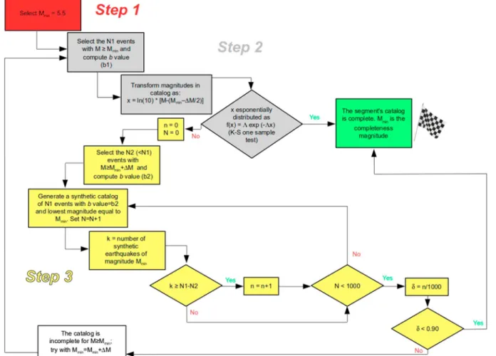
The minimum moment magnitude for which a seismic catalog can be considered complete (Mmin) is evaluated
in three steps (see flow chart in Figure 2). First, we set the first guess of completeness magnitude to Mmin= 5.5 for each subduction zone. Second, for each subduction zone, we verify the goodness of fit of the magnitudes equal to or larger than Mminusing a Kolmogorov-Smirnov test in the modified form proposed by Lilliefors
[1969]. If the G-R law holds, in fact, the magnitudes follow this exponential distribution [Aki, 1965; Marzocchi and Sandri, 2003]
f (x) = Λe−Λx, (1)
where x = Mw− (Mmin− ΔM∕2) +𝜖, ΔM is the width of the magnitude bin (in our case ΔM = 0.1), and the
summand𝜖 is a [−ΔM∕2, ΔM∕2] uniform random noise that mimics the magnitude uncertainty and that is necessary to remove ties in the data set. The null hypothesis of exponential distribution is rejected if the value of the test falls in the 1% tails of the distribution (the significance level is 0.01). The third step consists of verifying if the first bin (the one relative to Mmin) contains a significantly low number of earth-quakes compared to what expected by a G-R law. Specifically, we calculate the b value using a minimum magnitude equal to Mmin + ΔM, and then we generate 1000 synthetic catalogs with Mmin and the same number of data of the real catalog; finally, we calculate𝛿 = n∕N, where N is 1000 and n is the number of times in which the first bin (the one relative to Mmin) of the synthetic catalogs contains a number of
earthquakes larger than or equal to number of earthquakes in the real catalog. The parameter𝛿 is large when the synthetic catalogs show much more earthquakes with respect to the real catalog on the first bin, indicating a likely incompleteness of the catalog. The catalog is considered complete for Mw≥ Mminif the data set is not statistically significant from an exponential distribution or if𝛿 is smaller than 0.90. When the whole data set is analyzed, the G-R distribution is not rejected by the data with a significance level of 0.10, proving that the frequency-magnitude distribution of interplate earthquakes is well represented by the G-R law.
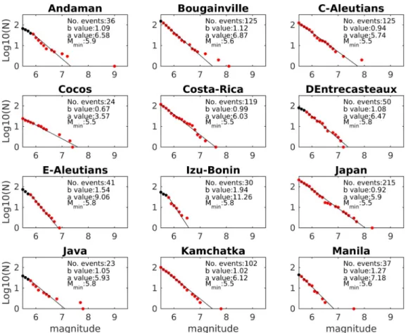
In Figure 3, we report the G-R of all subduction zones with at least 20 events having Mw≥ Mmin, and the Mmin
selected as above [Bender, 1983] (the influence of this choice on the final results is tested in the supporting information). Table 1 shows if the null hypothesis of exponential distribution (step 2) can be rejected with a significance level of 0.01, the parameter𝛿 described before, and the Mminvalues. From Table 1, we note that the exponential distribution is rejected at a 0.01 significance level only in S-Tonga. It is worth remarking that
Figure 2. Flow chart showing the procedure used to select, at a given subduction zone, the most appropriateMmin. Starting step is in the red box, and the procedure ends when reaching the green box. Different colors of the boxes indicate the three steps of the analysis described in the text.
for S-Tonga the first bin relative to Mmincontains more events than expected on average by a complete G-R
distribution; therefore, we conclude that the discrepancy from an exponential distribution is probably not due to an incompleteness of the seismic catalog.
To verify the stability of the results, we calculate the a and b values using a minimum magnitude equal to Mmin+ 0.1 and using Mmin= 6 for all subduction zones. We do not note any significant variation with respect to the values obtained using Mmincalculated here.
3.2. Estimating the a and b Values of the Gutenberg-Richter (G-R) Law
To calculate the a and b values with a sufficient accuracy and precision, we analyze only subduction zones with at least 20 interplate earthquakes above the completeness magnitude (Mmin) in each respective zone. After this selection, we have K = 34 (out of 62) subduction zones with enough data to estimate the a and b values (Figure 1). The b value is estimated applying the maximum likelihood estimation corrected for binned magnitudes [Marzocchi and Sandri, 2003]
b = 1
ln(10)[𝜇 − (Mmin− ΔM∕2)]
, (2)
where Mminis the threshold magnitude for completeness,𝜇 is the mean of the magnitudes recorded in the catalog larger or equal to the completeness magnitude Mmin, and ΔM is the binning width as above. In our
case, the list of Mminfor the various segments is provided in Table 1. The 1 sigma uncertainty on b value is
estimated through Page [1968]
Δb =√b N,
Figure 3. G-R relationships for the 34 selected subduction zones. Red stars show the cumulative relationships, for data
withMw≥ Mmin; black stars show the data below the completeness magnitude. The solid line is the best fitting line based on maximum likelihood estimates foraandbvalues. For each subduction zone, the computedaandbvalues are given, along withMmin, and the number of events withMw≥ Mmin. Other information are reported in Table 1.
where N is the number of interplate earthquakes in the catalog with magnitude larger or equal to Mmin. It is worth remarking that the uncertainty on the magnitude estimations does not affect the b value estimation [Marzocchi and Sandri, 2003].
The a value of the annual cumulative G-R law is estimated applying the maximum likelihood estimation to a Poisson process. In particular, Bender [1983] show that the equation for the noncumulative a0is
a0= Log ⎡ ⎢ ⎢ ⎢ ⎢ ⎣ n ∑ i=1 ki n ∑ i=1 e(−𝛽Mi) ⎤ ⎥ ⎥ ⎥ ⎥ ⎦ − Log(𝜏), (4)
where kiis the number of interplate earthquakes of binned moment magnitude Mi, Miis the center of the binned interval, n is the number of magnitude bins≥ Mmin,𝛽 = b ⋅ ln(10), and 𝜏 is the length of the catalog in years. The length of the catalog is the period January 1976 to December 2007 (𝜏 = 32) for all subduction zones, except for Andaman and Sumatra. In the latter zones, we compute this annual rate of earthquakes by considering only the events (and the consequent length of the catalog) from 1976 to the occurrence of the giant event (excluded) that is, respectively, until 2004 and 2005. In this way, we try not to alter the interplate earthquakes’ rate in these segments due to possible significant aftershock occurrence after giant events. The avalue of the annual cumulative G-R law is obtained integrating the noncumulative version of the GR law, i.e.,
a = Log [Mmax ∑ Mi=0 N(Mi) ] = Log [Mmax ∑ Mi=0 10a0−b⋅Mi ] , (5)
Figure 3. (continued)
where Miare the bins of magnitude from 0 to an arbitrary large Mmax(any reasonable choice of this
param-eter does not affect the results). The uncertainty on a values is estimated through error propagation by equations (4) and (5). In particular, the uncertainty on a is given by propagating the uncertainty on the b value and the statistical variability of the Poisson random variable ki.
The b values calculated for different subduction zones are reported in Figure 4a. Note that the use of a G-R distribution instead of a tapered distribution does not affect significantly the b value estimation; in fact, any reliable corner magnitude of each subduction zone is larger than the magnitudes reported in the seismic catalog used here [cf. Kagan and Jackson, 2013]; moreover, since there is no empirical evidence that the corner magnitude (if any) varies across the subduction zones, we assume that the presence of a corner magnitude does not affect significantly the analysis of a and b values. In Figures 4b and 4c, we plot also the distribution of a values and the relationship between a and b values for each subduction zone. The correlation between these two parameters is not a novelty [e.g., Stromeyer and Grünthal, 2015] and it will not be discussed here, but the correlation of the a value and b value with the propensity is of particular importance and it will be discussed later on.
For now, the most pressing scientific question is whether the b value variability is due to random chance or it shows statistically significant variations across the subduction zones. This aspect has important implications; if the b value is the same in all subduction zones, we may assume that giant interplate earthquakes occur more likely on subduction zones that have higher interplate seismicity rate. On the other hand, significant varia-tions of the b value imply that each subduction zone may have its own frequency-magnitude distribution which makes each subduction more or less prone to generate giant interplate earthquakes almost regardless the interplate seismicity rate. For this purpose, we test a null hypothesis which states that the set of all inter-plate earthquakes is a random sample from one single G-R distribution with the same b value. To this end, we first build the empirical G-R distribution with all the interplate earthquakes recorded in the 34 subduction zones with sufficient data; then, we select the completeness magnitude as the maximum of all the Mminout of
Figure 3. (continued)
achieving a b value equal to 0.942 (Figure 5a). We then carry out 10,000 simulations; in each simulation we (i) generate 34 synthetic catalogs (one for each subduction zone) with the same number of interplate earth-quakes as in the real catalogs and the same b value equal to 0.942 for all subduction zones, (ii) recalculate the b values of the 34 synthetic catalogs, and (iii) keep memory of the standard deviation of the 34 b values estimated from the synthetic catalogs and the difference between maximum and minimum of the 34 recal-culated b values. The result (Figure 5b) shows that the P value of the test (i.e., the probability to get the value of a random variable equal to or larger than the value observed in the real data, given the model under test; in this case a model that is based on a single b value) is much smaller than 0.01; specifically, the wide range of the observed interplate b values is significantly higher than the variation expected by chance. This result is surprising since the b value of the global seismicity was found to vary only in small geographic areas and among different tectonic regimes [Schorlemmer et al., 2005], and it shows overall that interplate seismicity may have different features. Note that this test implicitly assumes that the b value in each subduction zone does not have significant variations in the time interval considered (about 30 years).
3.3. The Propensity
We estimate the propensity to host giant interplate earthquakes (Ω) as the average annual rate of Mw≥ 8.5
earthquakes [Aki, 1965] for each one of the K subduction zones where we have calculated the b value; specifically,
Ωi≡ 𝜆i= 10ai−bi8.5, (6)
where aiand biare the parameters of the G-R relationship for the ith subduction. Figure 4c shows that the
propensity is inversely correlated with a and b, being high when a and b values are low. In Figure 1 and Table 1, we show the propensities for the subduction zones with enough data to calculate the b value. The range is more than 3 orders of magnitude, showing large variation in the propensity to host giant interplate earth-quakes. A correct interpretation of such a variability requires a careful evaluation of the uncertainty on the propensity given by equation (6). This will be done in the testing phase described in section 4.
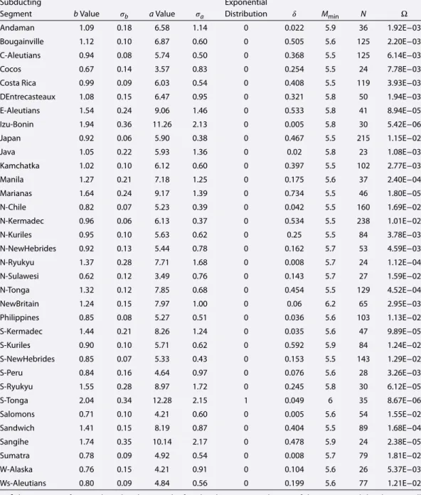
Table 1. Parameters and Standard 1 Sigma Errors of the G-R Law,Mmin, the Number of Data AboveMmin, and the PropensityΩ(i.e., Average Annual Rate) to Produce Giant Earthquakes for Each Subduction Zone Considereda
Subducting Exponential
Segment bValue 𝜎b aValue 𝜎a Distribution 𝛿 Mmin N Ω
Andaman 1.09 0.18 6.58 1.14 0 0.022 5.9 36 1.92E−03 Bougainville 1.12 0.10 6.87 0.60 0 0.505 5.6 125 2.20E−03 C-Aleutians 0.94 0.08 5.74 0.50 0 0.368 5.5 125 6.14E−03 Cocos 0.67 0.14 3.57 0.83 0 0.254 5.5 24 7.78E−03 Costa Rica 0.99 0.09 6.03 0.54 0 0.408 5.5 119 3.93E−03 DEntrecasteaux 1.08 0.15 6.47 0.95 0 0.321 5.8 50 1.94E−03 E-Aleutians 1.54 0.24 9.06 1.46 0 0.533 5.8 41 8.94E−05 Izu-Bonin 1.94 0.36 11.26 2.13 0 0.005 5.8 30 5.42E−06 Japan 0.92 0.06 5.90 0.38 0 0.467 5.5 215 1.15E−02 Java 1.05 0.22 5.93 1.36 0 0.02 5.8 23 1.08E−03 Kamchatka 1.02 0.10 6.12 0.60 0 0.397 5.5 102 2.77E−03 Manila 1.27 0.21 7.18 1.25 0 0.175 5.6 37 2.40E−04 Marianas 1.64 0.24 9.17 1.39 0 0.734 5.5 46 1.80E−05 N-Chile 0.82 0.07 5.23 0.39 0 0.042 5.5 160 1.69E−02 N-Kermadec 0.96 0.06 6.13 0.37 0 0.534 5.5 238 1.01E−02 N-Kuriles 0.95 0.10 5.63 0.62 0 0.25 5.5 84 3.78E−03 N-NewHebrides 0.92 0.13 5.44 0.78 0 0.162 5.7 53 4.59E−03 N-Ryukyu 1.37 0.28 7.71 1.68 0 0.008 5.7 24 1.12E−04 N-Sulawesi 0.62 0.12 3.49 0.76 0 0.143 5.7 27 1.59E−02 N-Tonga 1.32 0.12 7.85 0.68 0 0.454 5.5 129 4.52E−04 NewBritain 1.24 0.15 7.97 1.00 0 0.06 6.2 65 2.95E−03 Philippines 0.85 0.08 5.27 0.51 0 0.036 5.6 103 1.13E−02 S-Kermadec 1.44 0.21 8.26 1.24 0 0.035 5.6 47 9.89E−05 S-Kuriles 0.90 0.10 5.71 0.62 0 0.592 5.9 84 1.24E−02 S-NewHebrides 0.85 0.07 5.33 0.43 0 0.153 5.5 143 1.29E−02 S-Peru 0.84 0.16 4.64 0.97 0 0.076 5.6 28 3.26E−03 S-Ryukyu 1.55 0.28 8.97 1.72 0 0.245 5.8 30 6.12E−05 S-Tonga 2.04 0.34 12.28 2.15 1 0.049 6 35 8.67E−06 Salomons 0.71 0.10 4.21 0.60 0 0.005 5.6 54 1.55E−02 Sandwich 1.41 0.15 8.19 0.87 0 0.404 5.5 89 1.68E−04 Sangihe 1.74 0.35 10.14 2.17 0 0.478 5.9 24 2.38E−05 Sumatra 0.78 0.09 4.92 0.54 0 0.008 5.7 79 1.81E−02 W-Alaska 0.76 0.15 4.21 0.91 0 0.104 5.6 26 5.37E−03 Ws-Aleutians 0.80 0.09 4.84 0.56 0 0.199 5.6 77 1.21E−02
aThe meaning of𝛿is explained in the text. The fourth column reports the test of the exponential distribution null
hypothesis: a value of 0 means that the null hypothesis is not rejected at a significance level of 0.01, and a value of 1 means that the null hypothesis is rejected.
Finally, we also consider the case where the propensity accounts for the length of the subduction zone. In particular, in the supporting information section we redo all calculations and tests rescaling linearly the propensity of Table 1 with the length of the subduction zone R in kilometers [Heuret et al., 2011]; for this purpose, it suffices to rescale the annual cumulative a value, that is, equation (4) becomes
a0= Log ⎡ ⎢ ⎢ ⎢ ⎢ ⎣ n ∑ i=1 ki n ∑ i=1 e(−𝛽Mi) ⎤ ⎥ ⎥ ⎥ ⎥ ⎦ − Log(𝜏) − Log(R). (7)
Figure 4. (a) Distribution of thebvalue for the subduction zones with at least 20 interplate earthquakes withMw≥ Mmin. (b) Same as Figure 4a foravalues. (c) Plot ofb(xaxis) andavalues (yaxis), with 1 sigma error bars, and the propensity (same definition and color scale as used in Figure 1).
4. Are the Propensities Statistically Different and Meaningful?
In this section we investigate if and how much the model based on the propensities of equation (6) is able to explain the occurrence of giant interplate earthquakes since 1960 better than a reference model in which the probability of a subduction zone to host a giant interplate earthquake depends only on the earthquake
Figure 5. (a) G-R relationship using the 746 interplate earthquakes withMw≥ 6.2that occurred in the 34 segments with
enough data to compute the G-R parameters. Solid circles and stars show the not cumulative and cumulative number of events, respectively. The solid line is the best fitting line based on maximum likelihood estimates for the G-R parameters. (b) Test of the null hypothesis: thebvalue is constant among the subduction zones. The two curves in blue and red represent, respectively, the distribution of the 10,000 standard deviations and range (defined as the difference between the maximum and minimum) of the recalculatedbvalues from the synthetic catalogs. The vertical dashed lines are the same quantities obtained by the real 34 seismic catalogs. The associatedPvalue is the probability of observing a synthetic quantity equal to or higher than the real one.
Table 2. Giant Earthquakes (Mw≥ 8.5) That Occurred Since 1960 (Di Giacomo
et al. [2015] for the Earthquakes Before 1976, and Dziewonski et al. [1981] and Ekström et al. [2012] for the Earthquakes in the Period 1976 to Present)a
Event Location Year Mw
1 S-Chile 1960 8.6 2 S-Chile 1960 9.6 3 S-Kurile Islands 1963 8.5 4 E-Alaska 1964 9.3 5 Ws-Aleutians 1965 8.7 6 Andaman 2004 9.0 7 Sumatra 2005 8.6 8 Sumatra 2007 8.5 9 N-Chile 2010 8.8 10 Japan 2011 9.1 11 Sumatra 2012 8.6
aNote that the latter event in italics is not a thrust earthquake.
rate (i.e., the b value is the same across the subduction zones). This reference model can be parametrized in terms of reference propensities that are defined as
Ωref i ≡ 𝜆 ref i = 10 aref i −b ref×8.5 , (8)
where the bref= 0.942 for all subduction zones (see Figure 5) and the aref
i is the a value for the ith subduction
recalculated using breffor all subduction zones.
The testing data set is composed by out-of-sample giant earthquakes that occurred since 1960 [Di Giacomo et al., 2015] reported in Table 2. We consider this time window, because the earthquake magnitudes are likely affected by much larger uncertainties before that date [Hanks and Kanamori, 1979; Hough, 2013]. Among the events reported in Table 2, six subduction zones (Andaman, Japan, N-Chile, Kuril, Sumatra, and Ws-Aleutians) hosted L = 7 giant events that we assume to be interplate earthquakes; other three giant earthquakes occurred in subduction zones not considered here either because the scarce number of data does not allow us to calculate the propensity (E-Alaska 1964, S-Chile 1960), or not directly related to a subduction (the strike-slip Mw8.6 that occurred on 11 April 2012). Three interplate giant earthquakes occurred during the learning period
(two in Sumatra in 2005 and 2007 and one in Andaman subduction zone in 2004), but they were excluded by the setup of the model in order to consider them out-of-sample for the testing phase.
The analysis consists of two likelihood tests, which are aimed at comparing different aspects of our model (equation (6)) and the reference model (equation (8)). The first test verifies if the model of equation (6) pro-vides propensities significantly larger than the propensities of the reference model (equation (8)) where out-of-sample giant earthquakes occurred. The second test considers also the years and the subduction zones where no giant earthquakes occurred; in this way we test if a model, which provides higher propensities in the first test, is not simply forecasting much more giant earthquakes than expected. Both tests are rooted on stochastic simulations which aim at mimicking the uncertainty of the propensity caused by the limited data set used to calculate Ω. Specifically, in the first test we calculate the probability of occurrence Priand Prrefi for
each ith giant interplate earthquake. Priis the annual probability to observe the ith giant interplate
earth-quake calculated from the Poisson distribution and using the rate given by equation (6). Prref
i is calculated
using the rate given by equation (8). Then we calculate the observed log likelihood difference Δ𝓁 = 𝓁 − 𝓁ref= L ∑ i=1 [ Log(Pri) − Log ( Prrefi )], (9)
where L is the number of giant interplate earthquakes. The value of Δ𝓁 can be interpreted as the information gain of the model based on propensity with respect to the reference model [Vere-Jones, 1998]. Since the test-ing data set is composed by out-of-sample events, Δ𝓁 can be also interpreted in a Bayesian perspective as the Bayes factor [Kass and Raftery, 1995] that gives an indication of how much the data suggest that one model is better than the reference model. Of course, Bayesian and frequentist approaches have profound differences
Figure 6. (a) Cumulative distribution of the 10,000Δ𝓁s(equation (9)) obtained from synthetic catalogs assuming that theLgiant interplate earthquakes are generated according to the reference model of equation (8); (b) cumulative distribution of thePvalue obtained from each one of the 1000 reference models that have been built accounting for the uncertainty over theaandbvalues of the reference model (see text for more details).
in many aspects. Here we do not discuss them and present the results both from the Fisher frequentist view based on the P value—for which the lower the P value, the larger the probability of the null hypothesis to be wrong—and from a Bayesian perspective. To check if the observed Δ𝓁 can be explained by chance, we generate 10,000 synthetic catalogs containing L giant interplate earthquakes, assuming that these events are randomly generated according to the reference model. In other words, with the synthetic catalogs we quantify the variability of Δ𝓁 caused by the limited data set, assuming that the reference model is true. For each syn-thetic catalog we calculate the two log likelihoods as before and their difference, Δ𝓁s(see equation (9)), where
sindicates the sth synthetic giant interplate earthquakes’ catalog. In this case, the observed Δ𝓁 is indicative of a statistically better performance of the model based on equation (6) with respect to the reference model of equation (8) if the associated P value is low enough. Then, we also interpret the observed Δ𝓁 as the Bayes factor and we compare this number with the table at page 777 of Kass and Raftery [1995].
In Figure 6a we show the cumulative distribution of Δ𝓁sand the observed value of Δ𝓁 = 1.49. In this case
the information gain indicates that the average probability gain of the propensity model with respect to the reference model for the giant interplate earthquakes observed since 1960 is about 31 times larger. The P value obtained by simulations is 0.014 suggesting that the probability to observe the real Δ𝓁 is very low, if the reference model is true. We also rerun the same test taking into account explicitly the uncertainty on the propensities that are mostly caused by the limited data set. Specifically, we randomly sample 1000 b values
Figure 7. (a) As for Figure 6a but relative to the second test based on equation (10) and (b) as for Figure 6b but relative
to the second test based on equation (10).
from the normal distribution N(bref, var[bref]), where bref = 0.942 and var[bref] = 0.0012; we consider each
sample as the “true” b value that is used to generate one synthetic catalog for each subduction zone with the same number of earthquake as in the real catalog (so 34 synthetic catalogs for each b value sampled). From these synthetic catalogs we estimate Ωiand Ω(ref )i as before. Basically, we rerun the same test as before
comparing the Δ𝓁 = 1.49 of the real catalog with 1000 distributions of Δ𝓁s(i.e., 1000 P values). In Figure 6b
we see that in all simulations, the P value is always less than 0.03. In a Bayesian view, the Bayes factor is 101.49,
and this would lead to conclude that there is “strong” evidence in favor of the model based on propensities with respect to the reference model.
In the second test we consider the 1 year probability to observe a giant interplate earthquake in each subduction zone. In this case,
Δ𝓁 = 𝓁 − 𝓁ref= K ∑ i=1 𝜏′ i ∑ j=1 { Xij[Log(Prj) − Log ( Prref j )] + (1 − Xij) [ Log(1 − Prj) − Log ( 1 − Prref j )]} , (10) where𝜏′
iis the number of years since 1960 (excluding the years used to calibrate the model in the ith
subduc-tion zone) and Xijis 1 if a giant interplate earthquake occurred at the ith subduction zone in the jth year and
0 otherwise. Then the test is carried out as described before. In Figure 7a we show the cumulative distribution of Δ𝓁sand the observed value of Δ𝓁 = 1.30; this indicates that the average probability gain of the propensity
earthquakes observed since 1960 is about 20 times larger. The P value derived from simulations is 0.007 sug-gesting that the probability to get the observed Δ𝓁 is still low, if the reference model is true. As before, we take into account uncertainties caused by the limited data set following the same procedure described above; in all simulations the P value is always less than 0.02 (Figure 7b). In terms of Bayes factor (101.30), the
evi-dence in favor of the model based on propensity with respect to the reference model is strong. For the sake of checking the stability of the results, in the supporting information we show the same Figures 6 and 7, but using only subduction zones with at least 50 earthquakes (Figures S1 and S2), and rescaling the propensity with the length of the subduction zones (see equation (5) and Figures S3 and S4). The results are essentially the same presented here. To sum, the results of the two tests show that the model based on the propen-sity of equation (6) is better than a reference model based on a single b value (equation (8)) to forecast the out-of-sample interplate giant earthquakes.
As final consideration, we discuss the possible effects of aftershocks on the results. In our analyses we use the complete catalog to calculate the propensities without doing any attempt to remove possible aftershocks. The main reason is that any kind of declustering is necessarily arbitrary; in fact, an implicit assumption in most of declustering techniques is that earthquakes can be grouped in two distinct classes: main shocks and aftershocks. We argue that this sharp distinction does not have a sound physical motivation and it is strongly model dependent [e.g., van Stiphout et al., 2012]. Moreover, some declustering techniques alter the b value, and therefore, they may introduce a bias into the analysis. Nevertheless, we may wonder if the presence of possible aftershocks (loosely defined as earthquakes mostly triggered by previous earthquakes) could have induced the signal that we find in this paper. We think that this possibility is rooted on the unrealistic scenario where aftershocks occurred more frequently on subduction zones that do not experience any out-of-sample giant earthquake. Under this scenario, in fact, the presence of aftershocks leads to higher a and b values, lowering the propensity for that subduction zones. For this reason, we think that the presence of possible aftershocks cannot create the signal that we find into the data.
5. Discussion and Conclusions
The main result of this paper is that subduction zones seems to show marked differences in the propensity to produce giant interplate earthquakes. There are different possible explanations of the statistical evidence that we have found, and some of them are not rooted on the physical process generating giant earthquakes. For instance, the results can be due to a possible unconscious bias that can never be excluded when ana-lyzing data retrospectively, to a statistical fluctuation that appears significant while it is not (on average 1 out of 100 papers showing results with a statistical significance of 1% are not really showing any true physical signal), and to systematic bias of magnitude estimations that varies across the subduction zones [e.g., Kamer and Hiemer, 2015]. However, there is also (at least) one possible physical explanation of our results. In particular, although all subduction zones that we have considered are capable of producing giant earth-quakes [e.g., McCaffrey, 2008], they may have a different capability of producing giant interplate earthearth-quakes, and this capability is linked to different frequency-magnitude distributions for interplate seismicity among the subduction zones. This result differs from the results obtained analyzing the whole subduction seismicity [Kagan and Jackson, 2013], where the same frequency-magnitude distribution holds for all subduction zones. We argue that these results are not necessarily incompatible, but our results highlight that interplate seis-micity may have its own peculiarities and it is not a random sample of the whole seisseis-micity of a convergent margin. In particular, since the largest earthquakes are almost all interplate events, the analysis of interplate events may provide important clues to understand where they are more likely to occur.
If the results obtained here are caused by a real physical process, they pose new important challenges for seismologists and geodynamicists. For instance, one consequence of the results is that high-propensity subduction zones do not have necessarily high seismicity rate of interplate events. This implies that also sub-duction zones with small seismicity rates can have a large propensity to host future giant earthquakes. The occurrence of Mw≥ 8.5 events in E-Alaska (1964), S-Chile (1960), Colombia (1906), Nankai (1707), and Cascadia
(1700) may likely corroborate this view. The spatial variation of the b value implies that seismic energy is released by subduction zones in different ways, either via the occurrence of few large earthquakes or a higher number of smaller events. Such a diversity in the seismogenic behavior is likely linked to differences in the interplay between several tectonic parameters [e.g., Heuret et al., 2011] that may control different frictional properties of the plate interfaces. An analysis of possible cause-and-effect relationships between subduction
zones parameters and a and b values and propensity is beyond the scope of the present study. Interest-ingly, the fact that the subduction zones with the highest propensity of giant interplate events in the period 1976–2007 preferentially also hosted similar events that occurred before 1976 or after 2007 seems to indi-cate that the average friction properties remain overall constant through time; specifically, if the occurrence of a giant earthquake significantly modifies the friction properties, it would be unfeasible to observe a high propensity in a time period that follows the occurrence of a giant earthquake [e.g., Tormann et al., 2015]. The propensities reported in this paper are estimated by a limited data set and are affected by uncertainty (see Figure 4). This uncertainty is larger than the difference between adjacent propensity values of Figure 1; therefore, we do not aim at providing a precise rank of propensity for all subduction zones. Yet we show that the range of the propensities observed cannot be explained by the uncertainty due to the use of a limited data set. Moreover, we argue that some propensity values may be significantly affected by other parame-ters not considered here as, for instance, the lateral heterogeneities and extension of subduction thrust faults [Stubailo et al., 2012]; these (and others) parameters may contribute to make some subduction zone more or less prone to generate giant events. Nonetheless, we think that the results reported here may have a direct impact for global risk assessment. For instance, the results in Figure 1 show that some subduction zones such as, among others, North Chile and North Sulawesi have the highest predisposition to generate giant inter-plate earthquakes and their propensity is about 3.5 orders of magnitude larger than the propensity of other subduction zones like Izu-Bonin and S-Tonga (see Table 1).
References
Aki, K. (1965), Maximum likelihood estimate ofbin the formula log(N) = a − bMand its confidence limits, Bull. Earthquake Res. Inst. Univ.
Tokyo, 43, 237–239.
Bender, B. (1983), Maximum likelihood estimation ofbvalues for magnitude grouped data, Bull. Seismol. Soc. Am., 73, 831–851. Bird, P., and Y. Y. Kagan (2004), Plate-tectonic analysis of shallow seismicity: Apparent boundary width, beta, corner magnitude, coupled
lithosphere thickness, and coupling in seven tectonic settings, Bull. Seismol. Soc. Am., 94(6), 2380–2399.
Byrne, D. E., D. M. Davis, and L. R. Sykes (1988), Loci and maximum size of thrust earthquakes and the mechanics of the shallow region of subduction zones, Tectonics, 7, 833–857.
Di Giacomo, D., I. Bondár, D. A. Storchak, E. R. Engdahl, P. Bormann, and J. Harris (2015), ISC-GEM: Global instrumental earthquake catalogue (1900–2009): III. Re-computedMSandmb, proxyMW, final magnitude composition and completeness assessment, Phys. Earth Planet.
Inter., 239, 33–47.
Dziewonski, A. M., T.-A. Chou, and J. H. Woodhouse (1981), Determination of earthquake source parameters from waveform data for studies of global and regional seismicity, J. Geophys. Res., 86, 2825–2852, doi:10.1029/JB086iB04p02825.
Ekström, G., M. Nettles, and A. M. Dziewonski (2012), The global CMT project 2004–2010: Centroid-moment tensors for 13,017 earthquakes,
Phys. Earth Planet. Inter., 200–201, 1–9, doi:10.1016/j.pepi.2012.04.002.
Engdahl, E. R., R. Van Der Hilst, and R. Buland (1998), Global teleisismic earthquake relocation with improved travel times and procedures for depth determination, Bull. Seismol. Soc. Am., 88, 722–743.
Frohlich, C., and S. D. Davis (1999), How well constrained are well-constrainedT,B,Paxes in moment tensor catalogs?, J. Geophys. Res., 104, 4901–4910.
Fujiwara, H., S. Kawai, S. Aoi, N. Morikawa, S. Senna, K. Kobayashi, T. Ishii, T. Okumura, and Y. Hayakawa (2006), National seismic hazard maps of Japan, Bull. Earthquake Res. Inst. Univ. Tokyo, 81, 221–232.
Gutenberg, R., and C. F. Richter (1944), Frequency of earthquakes in California, Bull. Seismol. Soc. Am., 34, 185–188. Hanks, T. C., and H. Kanamori (1979), A moment magnitude scale, J. Geophys. Res., 84, 2348–2350.
Hardebeck, J. (2015), Stress orientations in subduction zones and the strength of subduction megathrust faults, Science, 349, 1213–1216. Hayes, G. P., D. J. Wald, and R. L. Johnson (2012), Slab1.0: A three-dimensional model of global subduction zone geometries, J. Geophys. Res.,
117, B01302, doi:10.1029/2011JB008524.
Heuret, A., S. Lallemand, F. Funiciello, C. Piromallo, and C. Faccenna (2011), Physical characteristics of subduction interface type seismogenic zones revisited, Geochem. Geophys. Geosyst., 12, Q01004, doi:10.1029/2010GC003230.
Hough, S. E. (2013), Missing great earthquakes, J. Geophys. Res. Solid Earth, 118, 1098–1108, doi:10.1002/jgrb.50083.
Ide, S. (2013), The proportionality between relative plate veolocity and seismicity in subduction zones, Nat. Geosci., 6, 780–784, doi:10.1038/NGEO1901.
Ide, S., G. C. Beroza, D. R. Shelly, and T. Uchide (2007), A scaling law for slow earthquakes, Nature, 447, 76–79. Isacks, B., J. Oliver, and L. R. Sykes (1968), Seismology and the new global tectonics, J. Geophys. Res., 73, 5855–5899.
Kagan, Y. Y. (1997), Seismic moment-frequency relation for shallow earthquakes: Regional comparison, J. Geophys. Res., 102, 2835–2852. Kagan, Y. Y., and D. D. Jackson (2011), Global earthquake forecasts, Geophys. J. Int., 184, 759–776.
Kagan, Y. Y., and D. D. Jackson (2013), Tohoku earthquake: A surprise?, Bull. Seismol. Soc. Am., 103, 1181–1194.
Kagan, Y. Y., P. Bird, and D. D. Jackson (2010), Earthquake patterns in diverse tectonic zones of the globe, Pure Appl. Geophys., 167, 721–741. Kamer, Y., and S. Hiemer (2015), Data-driven spatialbvalue estimation with applications to California seismicity: Tobor not tob, J. Geophys.
Res. Solid Earth, 120, 5191–5214, doi:10.1002/2014JB011510.
Kanamori, H. (1977), The energy release in great earthquakes, J. Geophys. Res., 82, 2981–2987. Kass, R. E., and A. E. Raftery (1995), Bayes factors, J. Am. Stat. Assoc., 90, 773–795.
Lilliefors, H. W. (1969), On the Kolmogorov-Smirnov test for the exponential distribution with mean unknown, J. Am. Stat. Assoc., 64, 387–389.
Marzocchi, W., and A. M. Lombardi (2008), A double branching model for earthquake occurrence, J. Geophys. Res., 113, B08317, doi:10.1029/2007JB005472.
Acknowledgments
All codes and data set used in this analysis are available upon request to the corresponding author. A com-pressed zip folder containing the files of the magnitudes for each subduc-tion zone can be downloaded here https://dl.dropboxusercontent.com/u/ 51584618/SupplementaryInformation/ dataeqs.zip. The authors thank Jeremy Zechar, Ian Main, the anonymous reviewers, and the Associate Editor; their comments and suggestions significantly improved the quality of the manuscript.
Marzocchi, W., and L. Sandri (2003), A review and new insights on the estimation of theb-value and its uncertainty, Ann. Geophys., 46, 1271–1282.
McCaffrey, R. (1994), Global variability in subduction thrust zone—Forearc systems, Pure Appl. Geophys., 142, 173–224. McCaffrey, R. (2008), Global frequency of magnitude 9 earthquakes, Geology, 36, 263–266.
Pacheco, J., and L. Sykes (1992), Seismic moment catalog for large shallow earthquakes from 1900 to 1989, Bull. Seismol. Soc. Am., 82, 1306–1349.
Page, R. (1968), Aftershocks and microaftershocks of the Great Alaska earthquake of 1964, Bull. Seismol. Soc. Am., 58, 1131–1168. Scholz, C. H. (2002), The Mechanics of Earthquakes and Faulting, 2nd ed., 471 pp., Cambridge Univ. Press, Cambridge, U. K.
Schorlemmer, D., S. Wiemer, and M. Wyss (2005), Variations in earthquake-size distribution across different stress regimes, Nature, 437, 539–542.
Stein, S., and E. Okal (2007), Ultralong period seismic study of the December 2004 Indian Ocean earthquake and implications for regional tectonics and the subduction process, Bull. Seismol. Soc. Am., 97, S279–S295.
Stromeyer, D., and G. Grünthal (2015), Capturing the uncertainty of seismic activity rates in probabilistic seismic-hazard assessments,
Bull. Seismol. Soc. Am., 105, 580–589.
Stubailo, I., C. Beghein, and P. M. Davis (2012), Structure and anisotropy of the Mexico subduction zone based on Rayleigh-wave analysis and implications for the geometry of the Trans-Mexican Volcanic Belt, J. Geophys. Res., 117, B05303, doi:10.1029/2011JB008631. Tormann, T., B. Enescu, J. Woessner, and S. Wiemer (2015), Randomness of megathrust earthquakes implied by rapid stress recovery after
the Japan earthquake, Nat. Geosci., 8, 152–158.
van Stiphout, T., J. Zhuang, and D. Marsan (2012), Seismicity declustering, Community Online Resource for Statistical Seismicity Analysis, doi:10.5078/corssa-52382934. [Available at http://www.corssa.org.]
Vere-Jones, D. (1998), Probability and information gain for earthquake forecasting, Comput. Seismol., 30, 248–263.
Wiemer, S., and M. Wyss (1997), Mapping the frequency-magnitude distribution in asperities: An improved technique to calculate recurrence times?, J. Geophys. Res., 102, 15,115–15,128.