HAL Id: hal-00317585
https://hal.archives-ouvertes.fr/hal-00317585
Submitted on 7 Sep 2004
HAL is a multi-disciplinary open access
archive for the deposit and dissemination of
sci-entific research documents, whether they are
pub-lished or not. The documents may come from
teaching and research institutions in France or
abroad, or from public or private research centers.
L’archive ouverte pluridisciplinaire HAL, est
destinée au dépôt et à la diffusion de documents
scientifiques de niveau recherche, publiés ou non,
émanant des établissements d’enseignement et de
recherche français ou étrangers, des laboratoires
publics ou privés.
GEOTAIL observation of tilted X-line formation during
flux transfer events (FTEs) in the dayside
magnetospheric boundary layers
M. Nowada, T. Sakurai, T. Mukai
To cite this version:
M. Nowada, T. Sakurai, T. Mukai. GEOTAIL observation of tilted X-line formation during flux
trans-fer events (FTEs) in the dayside magnetospheric boundary layers. Annales Geophysicae, European
Geosciences Union, 2004, 22 (8), pp.2907-2916. �hal-00317585�
Annales Geophysicae (2004) 22: 2907–2916 SRef-ID: 1432-0576/ag/2004-22-2907 © European Geosciences Union 2004
Annales
Geophysicae
GEOTAIL observation of tilted X-line formation during flux
transfer events (FTEs) in the dayside magnetospheric boundary
layers
M. Nowada1,2, T. Sakurai2, and T. Mukai1
1Institute of Space and Astronautical Science, Japan Aerospace Exploration Agency, Sagamihara, Kanagawa, Japan 2Department of Aeronautics and Astronautics, Tokai University, Hiratsuka, Japan
Received: 3 September 2003 – Revised: 4 March 2004 – Accepted: 8 April 2004 – Published: 7 September 2004
Abstract. The magnetic field and plasma structures dur-ing two successive crossdur-ings of the subsolar magneto-spheric boundary layers (i.e. MagnetoPause Current Layer (MPCL) and Low-Latitude Boundary Layer (LLBL)) under the southward-dawnward IMF are examined on the basis of the data obtained by the GEOTAIL spacecraft. A significant and interesting feature is found, that is, Flux Transfer Events (FTEs) occur in association with the formation of the tilted X-line. During the first inbound MPCL/LLBL crossing, the ion velocity enhancement (in particular, the Vl component negatively increases) can be observed in association with si-multaneous typical bipolar signature (positive followed by negative) in the Bncomponent. In addition, a clear D-shaped ion distribution whose origin is the magnetosheath can also be found in the dawnward direction. A few minutes later, the satellite experiences outbound MPCL crossing. The nega-tive enhancement of the Vmcomponent can be found as well as the positive enhancement of the Vl component. Simulta-neously, a typical bipolar signature with the polarity (nega-tive followed by posi(nega-tive) opposite that observed in the first encounter can also be observed. The ions from the magne-tosheath flow predominantly in the duskward direction, al-though the D-shaped ion distribution cannot be observed. These results indicate that the satellite initially observes one part of a reconnected flux tube formed by FTEs whose mag-netospheric side is anchored to the Southern Hemisphere. The ions confined in this partial flux tube are flowing in the south-dawnward direction. Then, the satellite observes the other part of the reconnected flux tube whose magnetospheric side is anchored to the Northern Hemisphere. The ions con-fined in this flux tube flow dominantly in the north-duskward direction. Furthermore, it can be considered that the second MPCL crossing is a direct cut through the diffusion region of FTEs because the LLBL is absent in the vicinity of the MPCL. On the basis of these results, it can be concluded that the satellite was passing near the tilted X-line. The
informa-Correspondence to: M. Nowada
tion obtained through this study is expected to be of great use in discriminating between the anti-parallel (steady-state) re-connection and tilted X-line models on the dayside MPCL.
Key words. Magnetospheric physics (Magnetopause, cusp, arid boundary layers; Magnetosheath; Solar wind-magnetosphere interactions)
1 Introduction
The structure and dynamics of the dayside magnetospheric boundary layer, that is, the MagnetoPause Current Layer (MPCL) and the Low-Latitude Boundary Layer (LLBL), are of great interest because they are important factors in de-termining the transport of the mass, momentum, and en-ergy of plasma from the magnetosheath (solar wind) into the magnetosphere. One of the important mechanisms of their transport into the magnetosphere is magnetic reconnection on the MPCL, which violates the magnetic frozen-in condi-tion. This magnetic reconnection on the MPCL originally was considered to be a large-scale and steady-state process (e.g. Petschek, 1964; Levy et al., 1964). However, Russell and Elphic (1978) found Flux Transfer Events (FTEs), which are the transient and patchy reconnection processes on the dayside MPCL, accompanied by small perturbations in the component of the magnetic field normal to the MPCL surface (Bn). The small magnetic field perturbations associated with FTEs are prominently of bipolar form, that is, positive fol-lowed by negative (hereafter referred to as positive/negative) or vice versa (negative/positive). Figure 1 shows the ba-sic schematic picture of FTEs on the northern side of the MPCL/LLBL provided by Russell and Elphic (1978). The intrinsic geomagnetic field lines directed northward (upward in the figure) are reconnected with the magnetosheath (solar wind) magnetic field lines directed south-duskward (right-downward in the figure). The resultant reconnected flux tube drapes around the magnetic field lines in the magnetosheath
2908 M. Nowada et al.: Tilted X-line formation during FTEs
Figure 1
Fig. 1. A schematic configuration of magnetic field lines for the Flux Transfer Events (FTEs) on the northern side of the MPCL/LLBL, taken from Russell and Elphic (1978). The flux tube is formed by reconnection of the intrinsic geomagnetic field lines directed northward (upward in figure) with the magnetosheath (solar wind) magnetic field lines directed south-duskward (right-downward in figure). This flux tube is prominent to the direction normal to the MPCL surface and drapes around the magnetosheath magnetic field lines. In addition, it is moving poleward due to mag-netic tension force, shown by the thick open arrow.
(solar wind) and moves poleward due to the magnetic ten-sion force, as shown by the open thick arrow. If the satellite encounters inbound crossing during these FTEs, the normal magnetic field component is first positive because the recon-nected flux tube, which is prominently in the direction nor-mal to the MPCL surface, is observed and then followed by negative due to the inward (tailward) movement of the recon-nected flux tube, in order to assimilate the magnetospheric flux tubes. As this FTE configuration is mainly formed on the northern side of the MPCL/LLBL, it is believed that the magnetospheric side of this reconnected flux tube is an-chored to the Northern Hemisphere. Oppositely, as the neg-ative/positive bipolar perturbation can mainly be found on the southern side of the MPCL/LLBL, it can be considered that the magnetospheric side of the reconnected flux tube is anchored to the Southern Hemisphere. These fundamental properties of FTEs are well understood based on further sta-tistical analysis using the magnetic field data obtained from ISEE-1 and -2 spacecrafts (e.g. Rijnbeek et al., 1982, 1984; Berchem and Russell, 1984). Thomsen et al. (1987) used the one- and two-dimensional ion and electron distribution func-tions obtained by ISEE-1 and -2 spacecrafts in order to
ex-amine the plasma properties during FTEs. They revealed that ion distribution within FTEs is a mixture of the cold compo-nents originating from the magnetosheath with the hot ions of the magnetospheric proper (i.e. the pancake-like ion dis-tribution). In this study, we have examined the magnetic field and plasma structures during FTEs within the MPCL/LLBL. As a result, it was confirmed that the tilted X-line is formed, and that the satellite passes near this. The results obtained through this study are expected to provide an important clue for discriminating between the anti-parallel (steady-state) re-connection and tilted X-line models on the dayside MPCL.
2 Observations 2.1 Instrumentations
This study is based on the magnetic field (Kokubun et al., 1994) and low-energy plasma moment (LEP) (Mukai et al., 1994) data obtained as the GEOTAIL spacecraft crossed the dayside MPCL on 29 January 1996. The time resolutions of the magnetic field and the plasma moment data are 3.0 s and 12.0 s, respectively. The LEP instrument covers the energy range from 32.0 eV/Q to 39.0 keV/Q. MPCL crossings are identified on the basis of the plasma moment data measured with sufficient counting statistics by means of a LEP-EA (Energy-per-charge Analyzer) instrument. Two successive MPCL crossings were observed during the intervals between 19:41:21 UT and 19:42:03 UT and between 19:45:42 UT and 19:47:12 UT. Simultaneous solar wind information was pro-vided by the WIND spacecraft.
2.2 Location of the observation
Figure 2 illustrates the one-day GEOTAIL orbit on 29 Jan-uary 1996, shown by the blue curve. The upper panel shows the GEOTAIL orbit projected onto a GSM-XY plane, and the lower panel shows it projected onto a GSM-XZ plane. The start (00:00 UT) and end (24:00 UT) points of the tra-jectory are marked by green and purple solid boxes, respec-tively. The locations of the average MPCL (Shue et al., 1998) and bow shock (Farris et al., 1991) are superimposed on the satellite trajectory. The red points show the location where GEOTAIL crosses the dayside MPCL/LLBL. The crossings of MPCL/LLBL are in the inbound (from magnetosheath to magnetosphere) and outbound (from magnetosphere to mag-netosheath) directions. The pass of the satellite on this day is indeed outbound, shown in this figure, but the MPCL crosses over the satellite due to its intrinsic motion. Therefore, we are examining the inbound and outbound MPCL crossings while on an outbound pass.
2.3 Overview of two MPCL/LLBL crossings
Figure 3 shows the summary plots during the interval of 12 min from 19:38:00 UT to 19:50:00 UT. From top to bot-tom panels, we show the intensity of the magnetic field, three components of the magnetic field, total ion bulk velocity,
M. Nowada et al.: Tilted X-line formation during FTEs 2909 three components of the ion bulk velocity in the
Bound-ary Normal Coordinate system (BNC) (Russell and Elphic, 1978) that are converted from the GSM coordinate system using the Minimum Variance Analysis (MVA), and ion num-ber density and its temperature. The coordinate transforma-tion of the magnetic field is made by
Bl Bm Bn = lx ly lz mxmymz nx ny nz Bx By Bz (1) ,
where (Bl, Bm, Bn) and (Bx, By, Bz) are the three compo-nents of the magnetic field in the BNC and the GSM coordi-nate systems, respectively. N is normal to the MPCL surface, the L direction is the projection of the GSM-Z component on the MPCL surface defined by N, and M completes the right-handed orthogonal system. The rotation matrices based on the magnetic field data when the satellite experiences two MPCL encounters are −0.042019 0.475494 0.878715 −0.299818 −0.844960 0.442891 0.953071 −0.244845 0.178065 (2) and 0.049932 0.165707 0.984910 −0.116330 −0.978463 0.170520 0.991955 −0.123089 −0.029580 , (3)
respectively. The matrices, shown by (2) and (3) are made by the data during periods from 19:40:57 UT to 19:42:12 UT and from 19:45:33 UT to 19:47:48 UT, respectively. A ro-tation matrix to transform the coordinate system on both the magnetic field and the ion velocity, shown by Fig. 3 is made based on the magnetic field data during 12 min from 19:38:00 UT to 19:50:00 UT. The observation time (UT) and the satellite locations in GSM coordinates (GSM-X, -Y and -Z) are also indicated at the bottom of the figure. The first inbound encounter of the MPCL can be observed during the time interval from 19:41:21 UT to 19:42:03 UT, as bracketed by solid lines. The MPCL crossing is identified by a clear jump of the north-south magnetic field component (almost Bl component in BNC coordinates) due to the Chapman-Ferraro current.
During the MPCL crossing, the Vl component changes its direction and the associated flow velocity also increases from 40.0 km/s to near 200 km/s. Simultaneously, the magnetic field intensity decreases abruptly from 60.0 nT to 40.0 nT. This suggests that the energy transfer from magnetic to ki-netic energy occurs within the MPCL. However, there are no outstanding variations of either ion number density or tem-perature.
Next, the satellite crossed the LLBL during the interval from 19:42:03 UT to 19:43:00 UT. The LLBL is the re-gion where the cold ions originating from the magnetosheath are dominant even though the satellite completely enters the magnetosphere (see Fig. 5). Although the ion bulk velocity
Figure 2
Fig. 2. The orbit of GEOTAIL on 29 January 1996 projected onto
the GSM-X and -Y (upper) and GSM-X and -Z (lower) planes. The start (00:00 UT) and end (24:00 UT) points of the trajectory are marked by green and purple solid boxes, respectively. The loca-tions where GEOTAIL crossed the MPCL/LLBL are marked by red points. The gray and black curves show the model bow shock (Far-ris et al., 1991) and magnetopause (Shue et al., 1998), respectively.
is 200 km/s or 250 km/s in the LLBL, the Vl negative en-hancement (-240 km/s) is very striking, marked by the blue oval. Simultaneous bipolar signature (positive/negative) can be found in the Bn component, suggesting the satellite en-counters a field-aligned current. The magnetic field inten-sity also increases slightly. These are typical signatures of the occurrence of the Flux Transfer Events (FTEs) (Rus-sell and Elphic, 1978). The ion number density continues to decrease and its temperature remains constant (0.3 keV) from the magnetosheath even though the satellite has already passed the MPCL. This is also evidence that the energy and mass of plasma from the magnetosheath (solar wind) pene-trate into the magnetosphere.
The second outbound encounter of the MPCL occurs from 19:45:42 UT to 19:47:12 UT, as bracketed by solid lines. The approximate duskward (eastward) enhancement (about
2910 M. Nowada et al.: Tilted X-line formation during FTEs
Figure 3
Fig. 3. A plot of GEOTAIL observations during the interval of 12 min from 19:38:00 UT to 19:50:00 UT on 29 January 1996. From top
to bottom: the magnetic field intensity (Bt), three components of the magnetic field (Bl, Bmand Bn), total ion bulk velocity (Vt), three
components of the ion bulk velocity (Vl, Vmand Vn) in the BNC coordinate system, ion number density (N ) and its temperature (T ). The
observation time (UT) and the satellite locations in GSM coordinates (GSM-X -Y and -Z) are also indicated at the bottom of the figure. The first MPCL and LLBL encounters and second MPCL crossing are indicated by solid lines, respectively.
M. Nowada et al.: Tilted X-line formation during FTEs 2911
WIND
Magnetic Field and Dynamic Pressure Plots
Year:
Date:
UT :
Bx[nT]
By[nT]
Bz[nT]
Bt[nT]
Pd[nPa]
UT GSM-X GSM-Y GSM-Z 0 0 0 0 01996
1/29
19:00 - 20:00
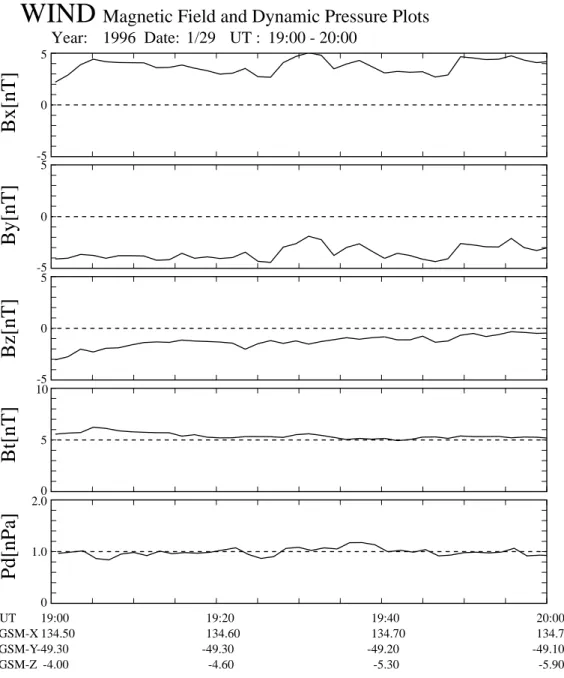
5 -5 5 -5 5 -5 10 5 2.0 1.0 19:00 134.50 -49.30 -4.00 19:20 134.60 -49.30 -4.60 19:40 134.70 -49.20 -5.30 20:00 134.70 -49.10 -5.90 Figure 4Fig. 4. Plots of the solar wind condition observed by the WIND spacecraft during a one-hour interval from 19:00:00 UT to 20:00:00 UT on
29 January 1996. From top to bottom: three components of the interplanetary magnetic field (IMF; Bx, Byand Bz) in GSM coordinates, the
intensity of IMF (Bt), and the solar wind dynamic pressure (1/2mprotonV2, m is assumed as the mass of proton). The observation time (UT)
and the satellite locations in GSM coordinates (GSM-X, -Y and -Z) are also indicated at the bottom of the figure.
−100 km/s) of the Vm component can be observed, marked by the green circle. The ion bulk velocity (particularly, the
Vlcomponent) is enhanced to 320 km/s, marked by the pink oval. Associated clear bipolar signature (negative/positive) due to a field-aligned current can also be seen in the Bn com-ponent. Simultaneous increase in the magnetic field intensity cannot be observed. The ion number density begins to in-crease and its temperature maintains as same value (0.3 keV) as that in the magnetosheath after experiencing the abrupt decrease from 4.3 keV to 0.8 keV.
2.4 Solar wind condition
The solar wind condition is also examined while GEOTAIL crosses the MPCL two times. Figure 4 shows a plot of the so-lar wind parameters obtained from the WIND spacecraft dur-ing the one-hour interval from 19:00:00 UT to 20:00:00 UT. The three components of the interplanetary magnetic field (IMF) in the GSM coordinate system, the intensity of IMF, and the solar wind dynamic pressure (1/2mprotonV2,m is
assumed as the mass of proton) are indicated from top to bottom. The observation time (UT) and the satellite loca-tions in GSM coordinates (GSM-X, -Y and -Z) are shown
2912 M. Nowada et al.: Tilted X-line formation during FTEsFigure 5
E-t Diagrams for Four Directions during
GEOTAIL MPCL/LLBL Crossings
1996/1/29: 19:41:21 UT – 19:42:03 UT
19:45:42 UT – 19:47:12 UT
Counts/Sample 5 10 20 50 100 200 500MPCL
Magnetosphere
LLBL
[keV]
19:38 19:40 19:42 19:44 19:46 19:48 19:50
Magnetosheath
MPCL
Magnetosheath
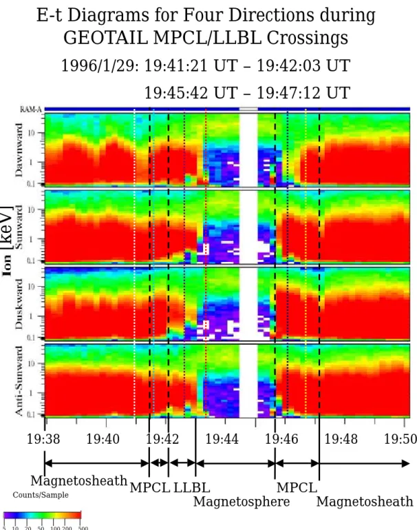
Fig. 5. Ion energy-time spectrograms for four directions (dawnward, sunward, duskward and antisunward directions) of two MPCLs and
LLBL crossings during the interval from 19:38:00 UT to 19:50:00 UT on 29 January 1996. The ion population from 5.0 counts/sample to 500 counts/sample is shown with the lower color bar. Two MPCL crossings are bracketed by broken lines.
in the bottom of the figure. During this interval, no large magnetic disturbance or abrupt increase (decrease) in the dy-namic pressure can be found. The directions of the IMF-Bx, -Byand -Bzcomponents are sunward, dawnward and south-ward, respectively. Next, we examined the plasma structures within the MPCL/LLBL under these solar wind conditions.
2.5 Overview of the plasma structures in the MPCL/LLBL
Figure 5 shows the Energy-time (E-t) diagrams of ions for four directions (dawnward, duskward, sunward and anti sun-ward (tailsun-ward)) when the satellite twice encountered the MPCL or LLBL. The horizontal and vertical axes indicate the observation time (UT) and energy of the ions (keV), re-spectively. The ion population is also shown by the lower
M. Nowada et al.: Tilted X-line formation during FTEs 2913
Figure 6
Ion Two- and One-Dimensional Distribution
Functions
Magnetosheath (19:40:59 UT) MPCL (19:41:36 UT) B-Cut LLBL (19:42:37 UT) (a) (b) (c) Gaps Gaps DAWNWARD DUSKWARD SUNWARD TAILWARD B 10 1 0 1 10 1500 km/s KeV/Q -1000 0 1000 [km/s] (FOR PROTONS) 10 1 0 1 10 KeV/Q -15.0 B⊥- Cut Log F (MKS UNIT) -8.0 -8.0 -1000 0 1000 [km/s] (FOR PROTONS) -15.0 DAWNWARD DUSKWARD SUNWARD TAILW A RD B 10 1 0 1 10 -9.0 B-Cut 10 1 0 1 10 KeV/Q -1000 0 1000 [km/s] (FOR PROTONS) -1000 0 1000 [km/s] (FOR PROTONS) -14.5 B⊥- Cut -14.5 10 1 0 1 10 10 1 0 1 10 KeV/Q -1000 0 1000 [km/s] (FOR PROTONS) -1000 0 1000 [km/s] (FOR PROTONS) -8.0 -14.5 -8.0 -14.5 DAWNWARD DUSKWARD SUNWARD TAILWARD B KeV/Q Log F (MKS UNIT) Log F (MKS UNIT) -9.0 KeV/Q B-Cut B⊥- Cut Magnetosphere (19:43:26 UT) (d) B-Cut 10 1 0 1 10 10 1 0 1 10 KeV/Q KeV/Q -1000 0 1000 [km/s] (FOR PROTONS) -1000 0 1000 [km/s] (FOR PROTONS) -8.0 -14.0 -8.0 -14.0 DAWNWARD DUSKWARD SUNWARD TAILWARD B B⊥- Cut Log F (MKS UNIT)MPCL (During Bipolar Signature) (19:46:05 UT) (e)
MPCL (After Bipolar Signature) (19:46:42 UT) (f) DUSKWARD DUSKWARD TAILWARD TAILWARD DAWNWARD DAWNWARD SUNWARD SUNWARD 10 1 0 1 10 -9.0 -9.0 10 1 0 1 10 KeV/Q KeV/Q B-Cut -1000 0 1000 [km/s] (FOR PROTONS) B⊥- Cut -1000 0 1000 [km/s] (FOR PROTONS) -14.5 -14.5 B-Cut -1000 0 1000 [km/s] (FOR PROTONS) B⊥- Cut -1000 0 1000 [km/s] (FOR PROTONS) -14.5 10 1 0 1 10 10 1 0 1 10 KeV/Q KeV/Q Log F (MKS UNIT) Log F (MKS UNIT) -8.0 -8.0 -14.5 B B
Fig. 6. Two- and one-dimensional ion distribution functions in the (a) magnetosheath (b) first MPCL, (c) LLBL, (d) magnetosphere, (e)
second MPCL during the interval in which the Bnbipolar signature can be found, and (f) second MPCL after the Bnbipolar signature
disappears. The hand panel shows the two-dimensional distribution function projected onto an equatorial plane. The upper, lower, left-and right-hleft-and sides correspond to the dawnward, duskward, sunward left-and antisunward (tailward) directions, respectively. The color code is assigned according to the logarithm of phase space density in units of m−6s3. The direction of the magnetic field lines projected onto an equatorial plane (shown with B) and the direction perpendicular to B are also superimposed on the distribution function. The middle and right-hand panels show the one-dimensional distribution functions cut along the B direction (B-cut) and the direction perpendicular to B (B⊥-cut), respectively. The lower, upper and left-hand axes provide the ion bulk velocity (km/s), its corresponding energy (keV/Q) and the
logarithm of the phase space density (m−6s3) which corresponds to the color of the color bar, respectively. The positive directions are shown by the arrowheads.
color scale, which ranges between 5.0 counts/sample and 500 counts/sample. From 19:38:00 UT to 19:41:21 UT, GEO-TAIL explored the magnetosheath. The ions in the sunward, duskward and antisunward directions are distributed up to 6.0 keV. However, the upper limit of the ion distribution in the dawnward direction abruptly decreases from 6.0 keV to 1.5 keV closer to the MPCL. Within the first MPCL from 19:31:21 UT to 19:42:03 UT, as bracketed by broken lines, the ions in all directions are distributed up to 6.0 keV. In the LLBL from 19:42:03 UT to 19:43:00 UT, although the lower limits of the dawnward and antisunward ion distribu-tions are almost the same as those in the magnetosheath and the MPCL, those of the sunward and duskward ion distribu-tions become higher from 0.1 keV to 0.5 keV. The ion pop-ulation in the duskward direction becomes smaller after the
Bnbipolar signature (about 19:42:39 UT) because the mag-netosheath low-energy ions dominantly flow in the
dawn-ward direction (see Fig. 6(c)). In the magnetosphere, from 19:43:00 UT to 19:45:42 UT, ions with energy lower than 6.0 keV cannot be found, and the energetic magnetospheric ions higher than 10.0 keV become the dominant ion compo-nent. The second encounter with the MPCL occurred during the interval from 19:45:42 UT to 19:47:12 UT, as bracketed by broken lines. No LLBL can be found because the cold ions originating from the magnetosheath do not penetrate into the magnetosphere beyond the MPCL. Within the sec-ond MPCL, the magnetosheath ions are predominantly dis-tributed up to 8.0 keV or 9.0 keV in the sunward and anti-sunward directions. These upper limits are slightly higher than those within the first MPCL. During the interval from 19:45:42 UT to 19:46:33 UT, in which the Bn bipolar sig-nature is just observed, the energy of the duskward ions is about 10.0 keV and the simultaneous dawnward ion popula-tion is much less than the ion populapopula-tions in other direcpopula-tions.
2914 M. Nowada et al.: Tilted X-line formation during FTEs After 19:46:33 UT, when the Bn bipolar signature
disap-pears, within the second MPCL, the energy of the duskward ions suddenly drops to about 5.5 keV. The dawnward ion population becomes larger and the ions are distributed up to 5.0 keV. After 19:47:12 UT, the satellite explores again the magnetosheath where the upper limits of the ion energy in all directions are between 8.0 keV and 9.0 keV.
2.6 Plasma distributions in magnetosheath, MPCL, LLBL, and magnetosphere
Figure 6 shows the two- and one-dimensional ion distribution functions obtained in the a) magnetosheath, b) first MPCL, c) LLBL, d) magnetosphere, e) second MPCL during the in-terval in which the Bn bipolar signature can be found, and f) second MPCL after the Bn bipolar signature disappears, which are marked by white, blue, purple, red, navy blue, and yellow dotted lines in the E-t diagram, respectively. The left-hand panel shows the two-dimensional ion distribution functions projected onto an equatorial plane. The upper, lower, left- and right-hand sides correspond to the dawn-ward, duskdawn-ward, sunward and antisunward (tailward) direc-tions, respectively. The direction of the magnetic field line (indicated by B) projected onto an equatorial plane and the direction perpendicular to B are also superimposed on the distribution function and shown by solid and broken arrows, respectively. The color code is assigned according to the log-arithm of the phase space density in units of m−6s3. The middle and right-hand panels show the one-dimensional dis-tribution functions cut along the B direction (hereafter, re-ferred to as the B-cut) and the direction perpendicular to B (the B⊥-cut), respectively. The horizontal, upper and vertical axes indicate the ion bulk velocity (km/s), its corresponding ion energy (keV/Q) and the logarithm of phase space density (m−6s3) which corresponds to the colors of the color bar, respectively. The blue curves show the one-count level of the ion distribution. The positive directions are shown by those of the arrowheads. The distribution of low-energy ions ( < 1.0 keV) in the a) magnetosheath is slightly elliptical but that of the high-energy ions is nearly circular (isotropic). The width of the low-energy part in the B⊥-cut is broader than that in the B-cut, as indicated by the open green box, and the widths of the higher energy parts in the B- and B⊥-cuts are comparable. The low- and high-energy ions of the b) MPCL are distributed isotropically and the B- and B⊥-cuts are similar. Comparing this distribution with that in the mag-netosheath, a larger amount of low-energy ions originating from the magnetosheath is distributed in the dawnward and duskward directions. In the c) LLBL where the Bn bipo-lar signature can be found, a clear D-shaped ion distribution can be seen in the dawnward direction, suggesting that the low-energy ions originating from the magnetosheath mostly flow in the dawnward direction (in the direction perpendic-ular to B). The D-shaped ion distribution in the LLBL has already been reported by Fuselier et al. (1991). The high-energy ions are distributed isotropically. In both B- and B⊥-cuts, there are clear gaps between the cold ions with
energy less than 0.3 keV and the magnetosheath ions (ap-pearing with a D-shaped ion distribution) with the peak at 0.7 keV. In the d) magnetosphere, although the low-density high-temperature ions are the dominant component, these plasma sheet ions cannot be found even in the high-energy tails of the distributions in the magnetosheath, MPCL and LLBL. In addition, the B- and B⊥-cuts are similar. Within the e) second MPCL crossing in the duration of the Bn bipo-lar signature, the low-energy ions from the magnetosheath are dominantly distributed in the duskward direction (along the B direction). The entire distribution of the components with energies higher than that of the ions from the magne-tosheath also shifted to the duskward direction. These can also be confirmed by the finding that the phase space density in the anti-parallel (negative) direction is much higher than that in the parallel (positive) direction on the B-cut. In the B⊥-cut, the perpendicular (positive) and anti-perpendicular (negative) distributions are symmetric to each other, although low-energy ions are entirely absent. This indicates that the high-energy ions are distributed isotropically in the direction perpendicular to B. Here, however, the D-shaped ion distri-bution and the associated gaps seen in d) cannot be observed, even though similar Bn bipolar signatures can be observed. After the Bnbipolar signature disappears, the distribution of ions is similar to those in the a) magnetosheath or b) MPCL. The low-energy part of the distribution is elliptical and in-clines to the dawn- and tailward directions, but the distribu-tion of high-energy ions is almost circular (isotropic). In the B- and B⊥-cuts, the distributions of the high-energy ions are similar, although the width in the low-energy part in the B-cut is narrower than that in the B⊥-cut (same part as indicated by open green box in a)).
3 Summary and discussions
In this study, we performed a detailed analysis of two suc-cessive MPCL crossings and a LLBL encounter based on the magnetic field, plasma moment data, ion E-t diagrams and ion two- and one-dimensional distribution functions. From the first MPCL to LLBL, the ion bulk velocity enhancement (in particular, the Vlcomponent) was observed even though the satellite location is near the subsolar region where the magnetosheath plasma flows very slowly. Associated bipo-lar signature (positive/negative) in the Bn component and the slight increase in the magnetic field intensity were also found. These were typical signatures of the Flux Transfer Events (FTEs) (Russell and Elphic, 1978).
Because the satellite experienced inbound crossing and the directions of simultaneous IMF-Byand -Bzcomponents were dawnward and southward, respectively, it can be con-sidered that the satellite was crossing the reconnected field lines (flux tube) formed by FTEs anchored to the Southern Hemisphere. On the E-t diagrams, the magnetosheath ions were dominant within the first MPCL and LLBL and no clear difference between them was seen.
M. Nowada et al.: Tilted X-line formation during FTEs 2915 However, in the LLBL, a clear D-shaped ion distribution
was observed in the direction perpendicular to B (dawnward direction) around the Bnbipolar signature. This suggests that the ions originating from the magnetosheath flowed in the direction perpendicular to the intrinsic magnetic field lines (B) (or the dawnward direction). Simultaneously, there was a clear gap at 0.3 keV in the one-dimensional ion distribu-tion, suggesting that low- and high-energy plasmas whose origins are entirely different were still not mixed completely in the reconnected flux tube. From this result, it can be con-sidered that this reconnected flux tube was relatively newly formed. Therefore, this ion distribution is inconsistent with the previous works of Thomsen et al. (1987). Within the first MPCL, the admixture of the high- and low-energy plasmas took place effectively, unlike that in the reconnected flux tube in the LLBL. This ion distribution is in rather good agree-ment with the result obtained by Thomsen et al. (1987).
Within the second MPCL, the negative Vmenhancement was observed in association with the positive enhancement of the Vl component. Simultaneous bipolar signature in the Bn component with the opposite polarity (negative/positive) to that in the former case can also be observed. Since the satel-lite experienced the outbound MPCL crossing, it can be con-sidered that the magnetospheric side of the reconnected flux tube formed by FTEs was anchored to the Northern Hemi-sphere. On the E-t diagram, the ions originating from the magnetosheath were the dominant component, and no clear boundary between the magnetosheath and MPCL was seen. However, the magnetosheath cold ions predominantly flowed in the direction perpendicular to B (duskward direction) dur-ing the interval when the Bnbipolar signature was observed, although no clear D-shaped ion distribution or associated gaps were found. This ion flow direction was exactly op-posite to that observed in the LLBL. After the Bn bipolar signature disappeared, the ion distribution was very similar to those within the first MPCL and the magnetosheath, sug-gesting that the satellite observed a part of the MPCL where the low- and high-energy ions were effectively mixed. The
Bnbipolar signature associated with FTEs can be observed in the LLBL on the first MPCL encounter but within the MPCL on the second one.
Regarding the result that the reconnected flux tube formed by FTEs was observed in all different regions, no clear rea-son can be found from the present data. However, it is signif-icant and interesting that the LLBL was absent in the vicin-ity of the second MPCL because the cold ions did not pene-trate into the magnetosphere before the MPCL crossing (see Fig. 5). The observation of the MPCL without the LLBL was made by Eastman et al. (1996) and they concluded that the MPCL without the LLBL can be observed when the satel-lite cuts directly through the diffusion region of the magnetic reconnection (FTEs). Therefore, it can be predicted that the satellite passed adjacent to the diffusion region of FTEs dur-ing the second MPCL crossdur-ing.
GSM-Y
GSM-Z
MPCL/LLBL
IMF
Fig. 7. A schematic illustration based on the results obtained from
this observation as well as the primary picture of FTEs provided by Russell and Elphic (1978) (see Fig. 1). This illustration is viewed from the Sun. Thin arrows show the intrinsic magnetic field lines within the MPCL/LLBL, which are directed northward. The thin red arrows are the IMF directed dawn-southward. MPCL/LLBL magnetic field lines reconnected with the IMF are shown by the combination of thick black and red arrows. The thick black ar-rows show the movement directions of two reconnected flux tubes. The broken curves indicate that the magnetospheric sides of the re-connected field lines are anchored to the Northern/Southern Hemi-spheres. The blue arrow and two green circles show the approxi-mate satellite orbit and locations of the two MPCL crossings.
4 Conclusion
From the results obtained in this study, the satellite is judged to have passed very close to where FTEs (magnetic reconnec-tion) were occurring. Conclusive evidence includes the ap-proximate east-west difference in the plasma flow (Vm) and the north-south velocity enhancement in the Vl component for each of the passes through the subsolar MPCL where the magnetosheath plasma flows very slowly. In addition, find-ings of the Bnbipolar signatures with two opposite polarities also become the clear evidence for the occurrence of FTEs. In Fig. 7, we show a schematic illustration, which is viewed from the Sun, produced on the basis of the results obtained in this observation as well as the primary picture of FTEs provided by Russell and Elphic (1978) (see Fig. 1). During two successive MPCL/LLBL encounters, the dawn-south di-rected IMF, shown by red arrows, reconnects with the intrin-sic magnetic field lines within the MPCL/LLBL that are di-rected northward, as shown by thin solid arrows. As a result, the tilted X-line formed by FTEs is observed, shown by two green circles and the blue arrow. Initially, the satellite expe-riences the inbound MPCL/LLBL crossing. Simultaneously, one part of a reconnected flux tube, shown by the combina-tion of thick red and black arrows, can be found. This partial reconnected flux tube is moving dawnward, shown by the thick arrow, and its magnetospheric side is anchored to the
2916 M. Nowada et al.: Tilted X-line formation during FTEs Southern Hemisphere, shown by the broken curve. The
satel-lite experiences the second outbound MPCL crossing with-out the LLBL due to a direct cut through the diffusion re-gion. Within the second MPCL, the other part of the recon-nected flux tube, shown by the combination of thick black and red arrows, can be observed. This part of the recon-nected flux tube is moving duskward, shown by the thick ar-row, and its magnetospheric side is nchored to the Northern Hemisphere, shown by the broken curve. The observation interval of the tilted X-line formed by FTEs is much shorter than that of the anti-parallel (steady-state) magnetic recon-nection at the MPCL (e.g. Nakamura et al., 1998). However, the results obtained through this observation are expected to be of great help in discriminating between the anti-parallel (steady-state) reconnection and tilted X-line models on the dayside MPCL.
Acknowledgements. We thank the GEOTAIL mission team for
pro-viding both the magnetic and plasma moment data.
Topical Editor T. Pulkkinen thanks S. Petrinec and another ref-eree for their help in evaluating this paper.
References
Berchem, J. and Russell, C. T.: Flux transfer events on the magne-topause: spatial distribution and controlling factors, J. Geophys. Res., 89, 6689–6703, 1984.
Eastman, T. E., Fuselier, S. A., and Gosling, J. T.: Magnetopause crossings without a boundary layer, J. Geophys. Res., 101, 49– 57, 1996.
Farris, M. H., Petrinec, S. M., and Russell, C. T.: The thickness of the magnetosheath: constraints on the polytropic index, Geo-phys. Res. Lett., 18, 1821–1824, 1991.
Fuselier, S. A., Klumpar, D. M., and Shelly, E. G.: Ion reflection and transmission during reconnection at the earth’s subsolar magne-topause, Geophys. Res. Lett., 18, 139–142, 1991.
Kokubun, S., Yamamoto, T., Acu ˜na, M., Hayashi, K., Shiokawa, K., and Kawano, H.: The Geotail magnetic field experiment, J. Geomag. Geoelect., 46, 7–21, 1994.
Levy, R. H., Petschek, H. E., and Siscoe, G. L.: Aerodynamic as-pects of the magnetospheric flow, AIAA J., 2, 2065–2076, 1964. Mukai, T., Machida, S., Saito, Y., Hirahara, M., Terasawa, T., Kaya, N., Obara, T., Ejiri, M., and Nishida, A.: The Low Energy Par-ticle (LEP) experiment onboard the GEOTAIL satellite, J. Geo-mag. Geoelect., 46, 669–692, 1994.
Nakamura, M., Seki, K., Kawano, H., Obara, T., and Mukai, T.: Reconnection event at the dayside magnetopause on January 10, 1997, Geophs. Res. Lett., 25, 2529–2532, 1998.
Petschek, H. E.: Magnetic field annihilation, AAS-NASA Sympo-sium on the Physics of Solar Flares, NASA Spec. Publ. SP-50, 425–439, 1964.
Rijnbeek, R. P., Cowley, S. W. H., Southwood, D. J., and Russell, C. T.: Observations of reverse polarity flux transfer events at the Earth’s dayside magnetopause, Nature, 300, 23–27, 1982. Rijnbeek, R. P., Cowley, S. W. H., Southwood, D. J., and Russell,
C. T.: A survey of dayside flux transfer events observed by ISEE 1 and 2 magnetometers, J. Geophys. Res., 89, 786–800, 1984. Russell, C. T. and Elphic, R. C.: Initial ISEE magnetometer results:
Magnetopause observations, Space Sci. Rev., 22, 681–715, 1978. Shue, J. -H., Song, P., Russell, C. T., Steinberg, J. T., Chao, J. K., Zastenker, G., Vaisberg, O. L., Kokubun, S., Singer, H. J., Detman, T. R., and Kawano, H.: Magnetopause location under extreme solar wind conditions, J. Geophys. Res., 103, 17 691– 17 700, 1998.
Thomsen, M. F., J. A. Stansberry, S. J. Bame, S. A. Fuselier, and J. T. Gosling, Ion and elecron velocity distributions within flux transfer events, J. Geophys. Res., 92, 12,127–12,136, 1987.