HAL Id: hal-00295237
https://hal.archives-ouvertes.fr/hal-00295237
Submitted on 25 Feb 2003
HAL is a multi-disciplinary open access
archive for the deposit and dissemination of
sci-entific research documents, whether they are
pub-lished or not. The documents may come from
teaching and research institutions in France or
abroad, or from public or private research centers.
L’archive ouverte pluridisciplinaire HAL, est
destinée au dépôt et à la diffusion de documents
scientifiques de niveau recherche, publiés ou non,
émanant des établissements d’enseignement et de
recherche français ou étrangers, des laboratoires
publics ou privés.
Strategies for measuring canonical tracer relationships in
the stratosphere
O. Morgenstern, J. A. Pyle
To cite this version:
O. Morgenstern, J. A. Pyle. Strategies for measuring canonical tracer relationships in the stratosphere.
Atmospheric Chemistry and Physics, European Geosciences Union, 2003, 3 (1), pp.259-266.
�hal-00295237�
www.atmos-chem-phys.org/acp/3/259/
Chemistry
and Physics
Strategies for measuring canonical tracer relationships in the
stratosphere
O. Morgenstern1, *and J. A. Pyle1
1Centre for Atmospheric Science, Chemistry Department, University, Cambridge, UK *present address: Max-Planck-Institut f¨ur Meteorologie, Hamburg, Germany
Received: 31 October 2002 – Published in Atmos. Chem. Phys. Discuss.: 13 November 2002 Revised: 12 February 2003 – Accepted: 14 February 2003 – Published: 25 February 2003
Abstract. A high-resolution simulation of stratospheric long-lived trace gases is subsampled in ways resembling var-ious commonly used measurement platforms. The result-ing measurements are analyzed with respect to whether they allow an accurate determination of stratospheric tracer re-lationships, as a prerequisite for a quantification of mixing processes from them. By varying the simulated locations, frequencies, and, in the case of satellite data, accuracies of the measurements we determine minimal requirements that the measurements need to satisfy in order to be suitable for a derivation of tracer relationships.
1 Introduction
Dynamics and chemistry in the stratosphere are dominated by the existence of well-mixed regions, separated by trans-port barriers (Haynes and Shuckburgh, 2000). Within each well-mixed region, longlived tracers form “canonical corre-lations”, i. e., unique, well-defined curves that can be used to infer one tracer, based on knowledge of another. In the pres-ence of transport barriers air is no longer well mixed across the barrier, leading to the occurrence of multiple canoni-cal correlations seen in observations and, recently, in model studies (Plumb et al., 2000; Piani et al., 2002; Morgenstern et al., 2002 and 2003). Typically, at any given time there are the winter or spring polar region, the northern and south-ern midlatitudes, and the tropics, each characterized by its own canonical correlation. Mixing across transport barriers, most notably occurring upon breakdown of the polar vortex, is therefore readily associated with a change in the canonical correlations. (Hence the focus here is on “cumulative” mix-ing on the timescale of a season; Morgenstern et al., 2003, rather than “instantaneous” mixing on the timescale of days; Morgenstern et al., 2002). An attempt to quantify mixing
Correspondence to: O. Morgenstern (morgenstern@dkrz.de)
processes in a global sense may therefore be based on as-sessing the canonical correlations at different times.
Within measurement campaigns a suite of different instru-ments is generally used to measure a range of tracers and physical parameters. These platforms and instruments dif-fer regarding their frequency of operation, coverage, mea-surement accuracy, the range of measured species, and not least, their cost. A commonly used technique is based on balloon-borne in situ measurements. At a relatively high unit cost and with a sparse data coverage balloon-borne instru-ments yield highly accurate data sometimes spanning a wide range of tracers. Other approaches rely on ground-based instruments. Usually a large number of measurements can be afforded, but the number of measured species may be small, and often measurements only yield column integrals or a poorly resolved profile. By contrast, aircraft measure-ments offer high accuracy and a potentially large number of species measured with great flexibility regarding the choice of flight path, but such measurements are expensive and lim-ited in altitude. Finally, satellite measurements offer the best coverage of all but at a high initial cost. New satellites will greatly expand the range of measured parameters, e.g. EN-VISAT and the upcoming EOS AURA satellites (Edwards et al., 1995; Bovensmann et al., 1999). Their greatest draw-back is of course the measurement accuracy, relative to in situ measurements, and their poorer horizontal and vertical reso-lution, especially in the lower stratosphere. Other kinds of instruments, e.g. balloon- and aircraft-borne remote-sensing instruments, can also be used. In the interest of brevity they are excluded from the following discussion; they could be included without any conceptual problems. In the following, also for brevity balloon- and aircraft-borne measurements are assumed to be in-situ. Generally within a measurement cam-paign all of these platforms are used in parallel, e.g. during the recent SOLVE/THESEO 2000 campaign (Newman et al., 2003).
260 O. Morgenstern and J. A. Pyle: Measurement strategies for tracer relationships different platforms must satisfy so that the state of the
at-mosphere, as represented by the canonical correlations, may be inferred from the measurements. In principle, to un-derstand mixing between northern polar and midlatitude re-gions, we require measurements sufficient to ‘recognize’ the two canonical correlations characterizing these two regions. To this end we subsample a high-resolution chemical trans-port model (CTM) integration in ways resembling the differ-ent platforms, and evaluate the canonical correlations from the resulting data. The resulting discussion as to the num-ber, type and location of necessary measurements should of course not be understood as a recommendation to discontinue most of the measurements efforts that are presently under-taken; the discussion could however influence measurement strategies employed in future campaigns.
2 The chemical transport model
The model used for the subsampling studies is based on the SLIMCAT model (Chipperfield, 1999), used here in the vari-ant described by Morgenstern et al. (2003). The model cal-culates the evolution of 12 longlived tracers, taking into ac-count photolysis and diagnosed distributions of the reactive radicals O(1D), OH, and Cl. It uses prescribed horizontal winds taken from the European Centre for Medium-Range Weather Forecasts (ECMWF) operational analyses. Vertical winds are computed using the MIDRAD formulation for di-abatic heating (Shine, 1987). Advection is calculated using the accurate Prather (1986) scheme. The model is formulated on 25 isentropic levels spanning the range between 349 and 2800 K of potential temperature at a horizontal resolution of about 1.9◦. The simulation is started in 1 October 1999, from a 6-months spinup integration at 2.8◦horizontal resolution. Model data are stored at 12:00 UTC every 48 h, referred to as the “model times”. Morgenstern et al. (2003) give more details of this model integration.
3 Definition of measurement strategies
3.1 “Groundbased” measurements
In an imaginary campaign sensors are placed at Ny ˚Alesund (78.9◦N, 11.9◦E), Kiruna (67.8◦N, 20.4◦E), Aire sur l’Adour (43.7◦N, 0.2◦E), and Iza˜na (28.3◦N, 15.6◦W), cov-ering polar to subtropical latitudes. Any single sounding is thought to instantaneously yield profiles of N2O,
CFC-11 (CFCl3), and CH3Br over the sites throughout the entire
model domain, omitting the bottom model level. Soundings are performed at every model time, i.e. 35 times between 15 January and 23 March 2000. Since such a high sampling frequency and the static arrangement of sensors are charac-teristic of groundbased instruments, we refer to this scenario as the “groundbased” campaign, even though in reality, of
course, groundbased measurements of the species in ques-tion would generally yield very poor or no vertical resolu-tion of the profile. The three source gases are chosen be-cause they cover a large range of different lifetimes, namely 120 years for N2O, 45 years for CFC-11, and 0.7 years for
CH3Br (World Meteorological Organization (WMO), 1999).
For CH3Br we need to add that tropospheric sinks, which
in nature dominate its budget, are ignored in the SLIMCAT model, so its “equivalent lifetime” (that ensues in the absence of the tropospheric OH-sink) in the model is at least 30 years (Morgenstern et al., 2003). A “reference” scenario is defined to include data from all 4 stations. By successively remov-ing stations from the record we will analyze the sensitivity of the results to the choice of locations where measurements are taken, and will distill a minimum set of stations that needs to be retained.
3.2 “Balloon-borne” campaign
In reality, the measurements described in Sect. 3.1 as “groundbased” could be performed using balloon-borne in-struments, but then the cost of the assumed high sampling frequency would be forbidding. (For a discussion of satellite measurements, see below). Therefore, in a “balloon-borne” campaign performed out of the remaining minimum set of stations we analyze the sensitivity of the results with respect to varying the frequency of the soundings within limits that are characteristic of real balloon-borne experiments. The pe-riod covered is the same as for the measurements of Sect. 3.1. 3.3 Airborne campaign
In an imaginary airborne campaign a plane, equipped with sensors measuring the above three tracers, flies a triangle from Zugspitze (47.4◦N, 11.0◦E) to Ny ˚Alesund, then on-wards to Iza˜na, and back to Zugspitze, starting at 15 January 2000, 12:00 UTC. The flight is repeated after 6 weeks, at 26 February 2000. The entire journey takes about 42 h. In do-ing so the plane remains on the 452 K isentropic model level, except every 2 h when it performs an instantaneous dive to the bottom of the model domain. The level is chosen be-cause it roughly corresponds to the maximum flight altitude of the NASA ER-2 research aircraft in Arctic winter condi-tions. The journey is repeated once after six weeks. In the interpolation of the model data to the flight tracks, the spatial coordinates are interpolated linearly. In time such a linear in-terpolation is not sensible because of the large gaps between model data times. We therefore only take the nearest model time for which model data are available, effectively associat-ing every measurement along the flight track with one of two different, successive model times.
In a further scenario we sample the model along the flight tracks of the ER-2 plane during the SOLVE/THESEO 2000 campaign, again associating every measurement with the nearest model time. During that campaign the ER-2
120 140 160 180 N2O [ppbv] 200 220 240 260 0 50 100 150 200 F11 [pptv] 120 140 160 180 200 220 240 260 N2O [ppbv] 0 1 2 3 4 5 6 CH 3 Br [pptv]
Fig. 1. Correlative tracer plots of F11 and CH3Br with N2O, based
on the reference scenario of groundbased measurements every 48 h, between 15 January and 23 March 2000. The coloured lines mark the 5th order regression polynomia through the midlatitude (violet) and polar-vortex (green) data. The scatter plot of the “measure-ments” shows an area of low measurement density separating the two curves.
formed a series of flights into the polar vortex and in mid-latitudes (Morgenstern et al., 2002; Newman et al., 2003).
3.4 Satellite-borne measurements
We sample the model at the positions and times of the UARS/HALOE instrument, again selecting the model time nearest to the measurements. The HALOE instrument does not actually measure any of the tracers of interest here, but it does measure other tracers (CH4, HF, HCl, H2O) that could
substitute for these. The data coverage of HALOE is typical of present (and future) solar occultation experiments; other satellite instruments could have been used instead, and, of course, emission instruments will sample near-globally each day. For HALOE CH4 measurements, the stated relative
measurement accuracy (taking into account noise and aerosol effects but disregarding systematic errors) is about 2%, on average (Russell and Remsberg, 2001). In an effort to simu-late noise associated with measurement inaccuracy, we will perturb the model interpolates with random noise of a range of assumed widths and determine how much noise can be tol-erated. If we assume that the precision of the measurements remains constant in time then only measurement noise, as described by the accuracy, will affect our ability to distin-guish different canonical correlations, representing different regions of the atmosphere, from each other.
120 140 160 180 N2O [ppbv] 200 220 240 260 0 50 100 150 200 F1 1 [p pt v] 120 140 160 180 N2O [ppbv] 200 220 240 260 0 1 2 3 4 5 6 CH 3 Br [p pt v] 120 140 160 180 200 220 240 260 N2O [ppbv] 0.2 0.4 0.6 0.8 ∆C H3 Br [p pt v]
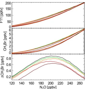
Fig. 2. Same as Fig. 1, but only the canonical correlations for the
measurements at (Iza˜na, Aire, Kiruna, Ny ˚Alesund; in black); (Aire, Kiruna, Ny ˚Alesund; red), (Aire, Kiruna; green), and (Kiruna; brown). The bottom plot shows the difference of the polar and midlatitude curves in CH3Br. The first three combinations yield
practically indistinguishable canonical curves. The brown curves representing Kiruna measurements only deviate somewhat in mid-latitudes and show a somewhat smaller spacing between the polar and midlatitude curves.
4 Results of the subsampling studies
4.1 The reference “groundbased” scenario
The correlations of CFC-11 and CH3Br with N2O
result-ing from the “reference” scenario described in Sect. 3.1 are displayed in Fig. 1. In this figure, to derive the “canonical correlations” we have fitted a 5th order polynomial through the entire correlative data set. The regression function di-vides the data into two subsets, each comprising roughly half of the measurements, lying above and below the regres-sion function. Again fitting two further regresregres-sion polynomi-als through these two halves yields two separate correlation functions which we refer to as “mid-latitude” and “polar”. (This procedure is adequate as long as the numbers of data points representing polar and mid-latitude conditions do not differ by orders of magnitude, which is not the case here.) Note that the curves closely follow the canonical correla-tions obtained from the full model data by Morgenstern et al. (2003). The canonical correlations thus defined are then readily compared to the results of different simulated mea-surement scenarios. Recall that, in order to be useful for identifying mixing, the measurement strategy must always
262 O. Morgenstern and J. A. Pyle: Measurement strategies for tracer relationships 120 140 160 180 N2O [ppbv] 200 220 240 260 0 50 100 150 200 F1 1 [p pt v] 120 140 160 180 N2O [ppbv] 200 220 240 260 0 1 2 3 4 5 6 CH 3 Br [p pt v] 120 140 160 180 200 220 240 260 N2O [ppbv] 0.2 0.4 0.6 0.8 ∆C H3 Br [p pt v]
Fig. 3. Same as Fig. 2, but with different balloon scenarios: The
reference case (Sect. 3.1; in black); 10 balloon soundings at Aire and Kiruna at 7-day intervals, starting 15 January 2000, 12:00 UTC (green); same, but only 3 balloon soundings at 28-day intervals (or-ange) ; same, but only 2 balloon soundings at a 42-day interval (red); same, but only 1 sounding at 15 January (brown). The first three scenarios yield indistinguishable canonical correlations.
allow these two relationships to be discerned.
4.2 Groundbased measurements with fewer stations
In a next step we assess the sensitivity of the “canonical cor-relations”, as derived from the reference scenario, to the re-moval of stations. The results are displayed in Fig. 2. Es-sentially, for example, removing Iza˜na and Ny ˚Alesund data (and leaving Kiruna and Aire sur l’Adour) does not apprecia-bly change the resulting canonical correlations at all. When only Kiruna data remain, the midlatitude curve becomes in-accurate. Out of the stations chosen here, only Kiruna is lo-cated near the boundary of the polar vortex so that, at dif-ferent times, both mid-latitude and polar air will pass over the station. Mixing events could possibly be identified using data from just this site. If we repeat the procedure for Aire sur l’Adour data only, then the analysis produces two nearly identical curves for every pair of tracers, both approximating the midlatitude canonical correlation (not shown). Measure-ments at this midlatitude site only would generally be insuf-ficient to identify mixing.
100 150 N2O [ppbv] 200 250
50
100
150
200
F1
1
[p
pt
v]
100
150
200
250
N
2O [ppbv]
0
1
2
3
4
5
6
C
H
3Br
[p
pt
v]
Fig. 4. “Aircraft” measurements, taken during one round trip (see
text) starting on 15 January 2000 (red). The black curves are the “reference” canonical correlations.
4.3 Balloon-borne campaigns
From the hypothetical, groundbased campaign (Sect. 4.2) we infer that polar and mid-latitude canonical correlations can be determined even if only data from Kiruna and Aire sur l’Adour are available. Next we assess how much we can reduce the frequency of measurements from these two sta-tions (mimicking a possible balloon coverage) while still re-taining accurately inferred canonical correlations. Figure 3 shows the results. Basically, the experiments indicate that the canonical correlations are extraordinarily robust with re-spect to thinning the data base. Even when the number of soundings is reduced to 3 soundings in Kiruna and a further 3 in Aire sur l’Adour, the canonical correlations are practi-cally identical to the reference scenario which comprises a total of 140 soundings. The “polar” curve is no longer iden-tifiable when only just one sounding is performed in Kiruna and one in Aire, because the Kiruna profile partially repre-sents midlatitude conditions on that date, 15 January. 4.4 Aircraft campaigns
Figure 4 shows the correlative tracer data of the first air-craft flight, starting 15 January 2000, along with the canon-ical correlations derived from the “reference” measurements (Sect. 4.1). The “isentropic” correlation (Morgenstern et al., 2002) corresponding to the flight level of 452 K is clearly discernible from Fig. 4. When the flight is repeated after 6 weeks (Fig. 5), essentially older air is encountered inside the vortex which is more depleted in source gases. However, on neither date does the aircraft properly sample significant portions of the midlatitude canonical correlations. This re-flects the fact that midlatitude air at aircraft altitudes is rela-tively young and therefore the longer-lived source gases have
100 150 N2O [ppbv] 200 250
50
100
150
200
F1
1
[p
pt
v]
100
150
200
250
N
2O [ppbv]
0
1
2
3
4
5
6
C
H
3Br
[p
pt
v]
Fig. 5. Same as Fig. 4, but for two round trips starting 15 January
and 28 February 2000.
experienced little depletion, leading to only a small range of mixing ratios characterizing this region. An analysis of mixing in this region is nevertheless quite possible (Morgen-stern et al., 2002, 2003). Note that balloon-borne measure-ments sampled in the model are also limited to altitudes be-low roughly 30 to 40 km, but this altitude range comprises substantially more of the ozone layer than an airplane would cover, and many commonly studied tracers drop to less than 10% of their tropospheric values at this height, e.g. CFC-11 and CH3Br.
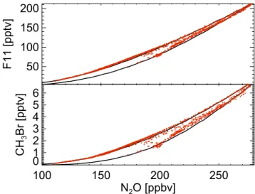
Figure 6 shows the tracer-tracer correlations if the model is subsampled along the flight tracks of the ER-2 during SOLVE/THESEO 2000. The aircraft nearly completely sam-pled the polar-vortex branches for CFC-11 and CH3Br
ver-sus N2O. The midlatitude branch is again only partially
cap-tured. A comparison with the real measurements for CFC-11 essentially confirms this result, even though perhaps in those data the midlatitude branch is less pronounced (Fig. 10 of Morgenstern et al., 2002). This allows us to conclude that the subsampling procedure adopted before captures the es-sential characteristics of stratospheric aircraft data, in that the polar-vortex canonical curves are more completely cov-ered by measurements than the mid-latitude ones. If mea-surements were taken in the tropics, an even smaller portion of the corresponding canonical correlations would be cov-ered.
4.5 Satellite measurements
As an example of a satellite instrument we consider the HALOE experiment. A solar occultation experiment like HALOE will not always have the Arctic within its view, un-like the more complete coverage provided by emission istru-ments. For example, between 15 January and 15 Febru-ary 2000, HALOE did not take any measurements north of
100 150 N2O [ppbv] 200 250
50
100
150
200
F1
1
[p
pt
v]
100
150
200
250
N
2O [ppbv]
0
1
2
3
4
5
6
C
H
3Br
[p
pt
v]
Fig. 6. Same as Fig. 4, but sampled along the flightpaths of the
ER-2 for the SOLVE campaign. Red dots are the measurements, the black solid lines are the results of the reference simulation.
41.5◦N. Correspondingly, the polar canonical correlations cannot be determined from this data. Between 15 Febru-ary and 15 March, however, points as far north as 63◦N came into view. Orbit and orientation of the satellite permit-ting, a satisfactory coverage of the mid- and high latitudes can thus be achieved. However, compared to ground- and balloon-based measurements discussed in Sects. 4.1 to 4.3 the HALOE data are strongly dominated by midlatitude mea-surements. This means that in the construction of the canon-ical correlations, midlatitude points need to be discriminated relative to polar measurements to achieve a good represen-tation of these curves (which by eye are discernible from scatterplots of the data). The discrimination is achieved by weighting the data with cos−10(φ), where φ is latitude. With this weighting, a visual inspection shows that the resulting re-gression polynomials reasonably represent the canonical cor-relations (Fig. 7). (A smaller weight given to high-latitude measurements moves the polar canonical correlation towards the midlatitude curve.) Compared to the equivalent figure for the groundbased scenario (Fig. 1), in relative terms the region between the two curves is considerably more densely popu-lated. This explains the large weighting that is necessary to move the polar curve towards what an observer would de-fine as the polar curve. Note that the HALOE data do not satisfy the requirement stated before (Sect. 4.1) that similar numbers of measurements must cover either side of the polar vortex barrier in order for the method presented here to give useful approximations to both canonical correlations.
The main problem with satellite-based data for studies of mixing of this kind is their poorer measurement accuracy, compared to in situ measurements. To simulate the feasibil-ity of extracting canonical correlations from satellite data, we take model profiles at all HALOE sampling locations north
264 O. Morgenstern and J. A. Pyle: Measurement strategies for tracer relationships 120 140 160 180 N2O [ppbv] 200 220 240 260 0 50 100 150 200 F1 1 [p pt v] 120 140 160 180 200 220 240 260 N2O [ppbv] 0 1 2 3 4 5 6 C H3 Br [p pt v]
Fig. 7. Scatterplots of model CFC-11 and CH3Br versus N2O,
sam-pled at the locations of the HALOE profiles, with a random pertur-bation of 0.5% on the model data (see text). Superimposed are the derived midlatitude (violet) and polar (green) curves.
of 21◦N, then multiply the profiles with random error tributions. The random error factors follow Gaussian dis-tributions centred at 1 with widths corresponding to the as-sumed measurement uncertainties of 0.05, 0.02, 0.01, and 0.005. Note that for example HALOE CH4 measurements
fall into this range (judging by the stated measurement ac-curacy, Sect. 3.4). The resulting canonical correlations, de-termined from all model “satellite” profiles, are displayed in Fig. 8.
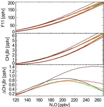
From the different “measurement accuracies” it is obvious that if the satellite-based sensor measures with a 5% accu-racy, in the lower stratosphere it is impossible to determine the canonical correlations from the model simulation with an accuracy necessary for an analysis of mixing. If that ac-curacy is improved to 2%, a reasonable approximation can be obtained throughout most of the model domain, and even more so at 1% and 0.5% accuracy. With the prescribed error characteristics the problem of determining the canonical cor-relations is most difficult to solve in the lower stratosphere where the separation between the two curves is small and the measurement uncertainty, in absolute terms, is large. It is also obvious that with the inclusion of a normally distributed error the polynomial approximation can undergo spurious changes in the sign of curvature which the unperturbed data do not exhibit; in this situation a different, more adequate way of approximating the canonical correlations may need to be employed.
The above discussion of necessary measurement accuracy of course also applies to in situ measurements. A full dis-cussion would however be beyond the scope of this paper.
120 140 160 180 N2O [ppbv] 200 220 240 260 0 50 100 150 200 F1 1 [p pt v] 120 140 160 180 N2O [ppbv] 200 220 240 260 0 1 2 3 4 5 6 CH 3 Br [p pt v] 120 140 160 180 200 220 240 260 N2O [ppbv] 0.2 0.4 0.6 0.8 1.0 1.2 1.4 ∆C H3 Br [p pt v]
Fig. 8. “Canonical correlations” derived from the model sampled
at the location of the HALOE profiles, with a random perturbation imposed on the model data. (brown) 5% normally distributed ran-dom error. (red) 2%. (orange) 1%. (green) 0.5%. (black) Reference “groundbased” canonical correlations.
5 Discussion of subsampling strategies and general con-cluding remarks
A key question associated with measurements of long-lived tracers is whether the data adequately define the canonical correlations that describe most of the stratosphere. From the analysis of model sampling, simulating various measurement platforms and strategies, canonical correlations can be cap-tured by very few measurements in locations representing the different stratospheric regions. For example, profile mea-surements in two locations representing the polar and mid-latitude environments can be sufficient to capture the corre-sponding canonical correlations. With a second set of mea-surements, taken after the vortex breakdown, mixing of for-mer vortex air can be derived, using an approach based on mixing lines (reviewed in Plumb et al., 2000) or techniques derived from that (e.g. Morgenstern et al., 2002).
The above statement depends on the degree to which stratospheric long-lived tracers form canonical correlations. In a highly transient situation such as the vortex breakdown, it can take some time before a well-defined mid-latitude canonical correlation is reestablished, e.g. during the bo-real spring of 2001 (Morgenstern et al., 2003). In this case clearly a larger number of measurements would be neces-sary. The winter of 1999/2000 was however characterized by a long-lasting vortex and little mixing across the vortex edge, in which case a small number of measurements can
capture the situation. For both winters the coverage pro-vided by, e.g. the primary Network for the Detection of Stratospheric Change (NDSC) stations (comprising 4 Arctic and 7 northern-midlatitude ones) (Kurylo and Zander, 2003) would have been more than sufficient to cover stratospheric development, provided some long-lived tracer profiles had been measured. In reality profile measurements are restricted to several stations measuring ozone and a few measuring aerosol and water vapour. Hence the data base presently gen-erated by the NDSC stations would actually be insufficient for an analysis of canonical tracer correlations.
The analysis of balloon-borne data suggests that with the strategy adopted here, namely performing launches at regu-lar, predefined intervals, one station at the boundary of the polar vortex may not be sufficient to cover both polar and midlatitude canonical correlations. If the strategy is modi-fied to take into account meteorological forecast information (as is done routinely in actual campaigns), and the launches are performed only when the forecast suggests a clean mid-latitude or polar profile, perhaps taking measurements only in one location like Kiruna might be sufficient. This would however seem to be a risky strategy, given the inaccuracy of forecasts and also the probability that such clean conditions may not occur at all. From the perspective of this paper such a strategy would introduce a degree of subjectivity; we have therefore not explored this route any further.
An aspect of satellite remote-sensing data not addressed thus far relates to the footprint size of the data, i.e. the size of a slab of atmosphere averaged to give the measurement. In the presence of sharp gradients of tracer features this av-eraging can suggest mixing between two reservoirs when in reality there is none. In contrast to real mixing, however, this “mixing” does not result in long-term changes of the canonical correlations. Footprint averaging would introduce a problem similar to measurement uncertainties, namely that in an extreme case canonical correlations may become in-distinguishable. A realistic simulation of this effect would require a model resolution better than that used here.
From a cost perspective a minimization of the number of in situ measurements is desirable. Satellites can provide a cov-erage unparalleled by any other platform, resulting – as far as long-lived tracers are concerned – in some redundancy in the data. However, this is achieved at the price of a compar-atively low resolution and, relatedly, a larger measurement inaccuracy than what is possible with in-situ measurements. Our analysis indicates that if the measurement inaccuracy significantly exceeds 2%, a construction of the canonical cor-relations from the data may become very difficult and am-biguous, especially in the lower stratosphere. This statement, valid for our model stratosphere of 1999/2000, depends on the degree of separation between the polar and mid-latitude canonical correlations, which may be subject to substan-tial interannual and inter-hemispheric variability. Generally, all conclusions drawn in this paper depend on how closely the simulation follows the real atmosphere. Morgenstern et
al. (2002, 2003) discuss in detail the simulation in question here, including model deficiencies. A compilation of obser-vational data compiled by Piani at al. (2002) indicates that possibly the separation of the polar and mid-latitude canon-ical correlations is even better in observations than in their model simulation (which closely parallels ours). This sug-gests that the permeabilility of the vortex barrier is lower in reality than in the model, as a consequence of transport errors and numerical diffusion. This would of course only corrobo-rate the findings of this paper.
Nevertheless, the analysis stresses the need to have rela-tively few but highly accurate instruments in place, deployed just a few times during the course of a season. With such a strategy it is already possible to monitor the gross devel-opment of the canonical correlations and hence, perhaps in conjunction with a modelling effort, to quantify the effects of mixing resulting in the observed changes.
Acknowledgements. The British Atmospheric Data Centre is
ac-knowledged for providing access to the ECMWF analyses. OM was supported by the European Commission under grant EUK2-CT-1999-CO049 within the SAMMOA project. We acknowledge support by the UK Natural Environment Research Council (NERC) within the UK Universities Global Atmospheric Modelling Pro-gramme (UGAMP) under grant NER/A/S/2000/00512. The Centre for Atmospheric Science is a joint initiative of the Departments of Applied Mathematics and Theoretical Physics and of Chemistry.
References
Bovensmann, H., Burrows, J. P., Buchwitz, M., Frerick, J., No¨el, S., and Rozanov, V. V.: SCIAMACHY: Mission objectives and measurement modes, J. Atmos. Sci., 56, 127–150, 1999. Chipperfield, M. P.: Multiannual simulations with a
three-dimensional chemical transport model, J. Geophys. Res., 104, 1782–1805, 1999.
Edwards, D. P., Gille, J. C., Bailey, P. L., and Barnett, J. J.: Selec-tion of sounding channels for the high-resoluSelec-tion dynamics limb sounder, Appl. Opt., 34, 7006–7018, 1995.
Haynes, P., and Shuckburgh, E.: Effective diffusivity as a diagnostic of atmospheric transport. 1. Stratosphere, J. Geophys. Res., 105, 22,777–22,794, 2000.
Kurylo, M. J., and R. J. Zander, Network for the Detection of Strato-spheric Change (NDSC), www.ndsc.ncep.noaa.gov, 2003. Morgenstern, O., Pyle, J. A., Iwi, A. M., Norton, W. A., Elkins,
J. W., Hurst, D. F., and Romashkin, P. A.: Diagnosis of mixing between middle latitudes and the polar vortex from tracer-tracer correlations, J. Geophys. Res., 107(D17), 4321, doi:10.1029/2001JD001224, 2002.
Morgenstern, O., Lee, A. M., and Pyle, J. A.: Cumulative mixing in-ferred from tracer-tracer correlations, J. Geophys. Res., in press, 2003.
Newman, P. A., Harris, N. R. P., and Adriani, A., et al.: An overview over the SOLVE/THESEO 2000 campaign, J. Geophys. Res., in press, 2003.
Piani, C., Norton, W. A., Iwi, A. M., Ray, E. A., and Elkins, J. W.: Transport of ozone-depleted air on the breakup of the
strato-266 O. Morgenstern and J. A. Pyle: Measurement strategies for tracer relationships
spheric polar vortex in spring/summer 2000, J. Geophys. Res., 107(D20), 8270, doi:10.1029/2001JD000488, 2002.
Plumb, R. A., Waugh, D. W., and Chipperfield, M. P.: The effects of mixing on tracer relationships in the polar vortices, J. Geophys. Res., 105, 10 047–10 062, 2000.
Prather, M. J.: Numerical advection by conservation of second order moments, J. Geophys. Res., 91, 6671–6681, 1986.
Russell, J. M. III and Remsberg, E. E.: Halogen Occultation Exper-iment (HALOE) Home Page, haloedata.larc.nasa.gov, 2001. Shine, K.: The middle atmosphere in the absence of dynamical heat
fluxes, Q. J. R. Meteorol. Soc., 113, 603–633, 1987.
World Meteorological Organization: Scientific Assessment of Ozone Depletion, 1998, Report No. 44, Geneva, 1999.