HAL Id: hal-00317780
https://hal.archives-ouvertes.fr/hal-00317780
Submitted on 22 Dec 2004
HAL is a multi-disciplinary open access
archive for the deposit and dissemination of
sci-entific research documents, whether they are
pub-lished or not. The documents may come from
teaching and research institutions in France or
abroad, or from public or private research centers.
L’archive ouverte pluridisciplinaire HAL, est
destinée au dépôt et à la diffusion de documents
scientifiques de niveau recherche, publiés ou non,
émanant des établissements d’enseignement et de
recherche français ou étrangers, des laboratoires
publics ou privés.
Studies of medium scale travelling ionospheric
disturbances using TIGER SuperDARN radar sea echo
observations
L.-S. He, P. L. Dyson, M. L. Parkinson, W. Wan
To cite this version:
L.-S. He, P. L. Dyson, M. L. Parkinson, W. Wan. Studies of medium scale travelling ionospheric
disturbances using TIGER SuperDARN radar sea echo observations. Annales Geophysicae, European
Geosciences Union, 2004, 22 (12), pp.4077-4088. �hal-00317780�
Annales Geophysicae (2004) 22: 4077–4088 SRef-ID: 1432-0576/ag/2004-22-4077 © European Geosciences Union 2004
Annales
Geophysicae
Studies of medium scale travelling ionospheric disturbances using
TIGER SuperDARN radar sea echo observations
L.-S. He1, *, P. L. Dyson1, M. L. Parkinson1, and W. Wan2
1Department of Physics, La Trobe University, Bundoora 3086, Australia
2Institute of Geology and Geophysics, Chinese Academy of Science, Beijing 100029, P. R. China *now at Department of Physics, University of Alberta, Edmonton, Canada
Received: 27 October 2003 – Revised: 13 August 2004 – Accepted: 3 September 2004 – Published: 22 December 2004
Abstract. Seasonal and diurnal variations in the direction of
propagation of medium-scale travelling ionospheric distur-bances (MSTIDs) have been investigated by analyzing sea echo returns detected by the TIGER SuperDARN radar lo-cated in Tasmania (43.4◦S, 147.2◦E geographic; −54.6◦3). A strong dependency on local time was found, as well as significant seasonal variations. Generally, the propagation direction has a northward (i.e. equatorward) component. In the early morning hours the direction of propagation is quite variable throughout the year. It then becomes predominantly northwest and changes to northeast around 09:00 LT. In late fall and winter it changes back to north/northwest around 15:00 LT. During the other seasons, northward propagation is very obvious near dawn and dusk, but no significant north-ward propagation is observed at noon.
It is suggested that the variable propagation direction in the morning is related to irregular magnetic disturbances that occur at this local time. The changes in the MSTID propaga-tion direcpropaga-tions near dawn and dusk are generally consistent with changes in ionospheric electric fields occurring at these times and is consistent with dayside MSTIDs being gener-ated by the Lorentz force.
Key words. Ionosphere (ionospheric disturbances; wave
propagation; ionospheric irregularities; signal processing)
1 Introduction
The ionospheric manifestations of atmospheric gravity waves (AGWs) are called travelling ionospheric disturbances (TIDs) (Munro, 1958) and medium-scale TIDs (MSTIDs) of sufficient amplitude and appropriate wavelength which cause focusing and defocusing of HF radio waves reflected at oblique incidence to the ionosphere. As a consequence, Su-perDARN radars detect quasi-sinusoidal variations in ground echo power which change in time as MSTIDs propagate (e.g.
Correspondence to: L.-S. He
Samson et al., 1989, 1990; Bristow et al., 1994, 1995, 1996, 1997; Huang et al., 1998a, b; Hall et al., 1999; Sofko and Huang, 2000; MacDougall et al., 2000). The Tasman Inter-national Geospace Environment Radar (TIGER) is located on Bruny Island, Tasmania (Dyson and Devlin, 2000), and like other SuperDARN radars, it can be used to study the oc-currence of medium-scale AGWs propagating in the thermo-sphere. Since TIGER’s footprint maps almost entirely over the Southern Ocean, we use the term “sea echoes” to refer to the echoes backscattered from the Earth’s surface.
Many data analysis methods have been developed to de-termine MSTID and MSAGW parameters (such as the phase velocity, azimuth, and wavelength) from different types of radio observations (e.g. Briggs, 1968a, 1968b; Tsutsui et al., 1984; Crowley et al., 1987; Shibata, 1987; Wan et al., 1996). Briggs (1968a) developed a correlation analysis to calculate the ionospheric disturbance velocity. Tsutsui et al. (1984) developed a cross spectral Fourier transform technique to de-termine wind velocity from an HF radar array, and Shibata (1987) and Wan et al. (1996) applied the maximum entropy method in their MSTID studies using radio systems. In an-alyzing SuperDARN observations to detect MSTID excita-tion sources, Samson et al. (1990) applied a cross-spectral analysis method (“MUSIC”) to time series obtained at dif-ferent range gates of the Goose Bay radar.
The statistical characteristics of MSTIDs have been stud-ied by several investigators. Using nine years of observa-tions, Munro (1958) found that daytime MSTIDs travelled toward the northeast in the Southern Hemisphere winter. Us-ing SuperDARN HF radar data, Bristow et al. (1996) found MSTIDs had maximum occurrence in winter. Ogawa et al. (1987) also concluded the existence of a seasonal vari-ation and indicated that there is a diurnal varivari-ation with max-imum MSTID occurrence between 14:00 and 16:00 LT, and a secondary maximum around midnight.
At high latitudes, energy deposition by Joule heating, the Lorentz force, and auroral particle precipitation, are re-garded as possible source mechanisms (e.g. Chimonas and Hines, 1970; Francis, 1974; Richmond, 1978). The relative
4078 L.-S. He et al.: Studies of medium-scale travelling ionospheric disturbances
15
Figures
Fig. 1
.
Fig. 2
Fig. 1. Coordinates system used for wave vector calculation in this
paper.
contributions to the generation of TIDs of the Lorentz force and Joule heating associated with the auroral electrojets have also been studied for several decades (e.g. Chimonas and Hines, 1970; Hunsucker, 1977; Brekke, 1979; Jing and Hun-sucker, 1993). Chimonas and Hines (1970) suggested that whether the Lorentz force or Joule heating was the more im-portant effect could not readily be decided due to the un-certainty of the ratio representing their relative importance. However, some investigators (e.g. Francis, 1975) regard the Lorentz force acting on auroral electrojet currents to be the dominant source. Jing and Hunsucker (1993) concluded from theoretical studies that the Lorentz force tends to gen-erate MSAGWs while the Joule heating dominates the exci-tation of large-scale AGWs (LSAGWs).
In this paper, an analysis method, based on the Fast Fourier Transform (FFT), will be developed and applied to Super-DARN observations to study MSTIDs. The relationship be-tween UT and local time (LT) changes significantly across the TIGER footprint. Nevertheless, for most purposes it is sufficiently accurate to use the relationship, LT≈UT+10 h.
2 Data analysis methods
The primary aim in this study was to determine phase ve-locities and azimuths of MSTIDs propagating through the TIGER field of view. This required the development of a method for determining MSTID frequencies (or periods) and wavelengths (or wave numbers) from time series of sea echo power. Sea echoes were selected using the standard Super-DARN analysis algorithm which identifies “ground echoes” as those with low line-of-sight Doppler velocities and spec-tral widths, typically less than 50 m s−1and 20 m s−1, respec-tively. This algorithm is usually very effective in separating sea echoes from ionospheric echoes. The radar footprint or field of view can be divided into “observation cells”, where an observation cell is defined as a specific range gate along
15
Figures
Fig. 1
.
Fig. 2
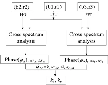
Fig. 2. Flow chart of FFT cross-spectral analysis method used to
determine MSTID wave numbers from TIGER SuperDARN radar observations. A specific observation cell in the TIGER’s field of view is identified by beam number bi and range cell rj, where i=0,
1, 2, . . . , 15; j =1, 2, . . . , 75. The time series of echo power at three observation cells is then used to determine kxand ky.
a particular azimuthal beam. In normal operation the radar scans 75 range gates along 16 azimuthal beams, providing up to 1200 possible observation cells.
The MSTID frequencies were determined using FFT cross-spectral analysis of time series of 4 h in duration. MSTIDs were detected as they passed through a single ob-servation cell by stepping the basic 4-h time window at ten-minute intervals through longer data sequences obtained at a single observation cell. Because of the finite coherency lengths of MSTIDs, increasing or decreasing the duration of the basic time-series window increases the sensitivity of the analysis to waves of longer or shorter periods, respectively. The frequency resolution is also greater for longer time se-ries. MSTIDs typically have periods of 20–50 min and last for just a few cycles and so the effect of one MSTID at a sin-gle range gate may last from about one hour or longer. Thus choosing the length of the basic time window for FFT anal-ysis is something of a compromise and the 4-h window was chosen as an appropriate window after preliminary investiga-tions using different window lengths. In the normal operation mode TIGER completes entire scans of all 16 radar beams at 1- or 2-min intervals, providing a more than adequate sam-pling rate of MSTID variations.
At any given time sea echoes are observed at only a sub-set of the 1200 possible observation cells, so the first stage of the analysis was to identify all observation cells providing time series of sea echoes with a duration of at least a signif-icant fraction of the 4 h. These time series were then used to identify any significant periodic variations occurring at each cell that were consistent with being MSTIDs. This was done by first converting each 4-h time series of sea echo power to a time series of echo amplitude which was then subjected to FFT analysis to determine the power spectrum. For a given
L.-S. He et al.: Studies of medium-scale travelling ionospheric disturbances 4079
16
Fig. 3
Fig. 4
A
B
C
A
B
C
A
B
C
C
B
D
B
C
D
B
C
D
1
3
5
2
4
6
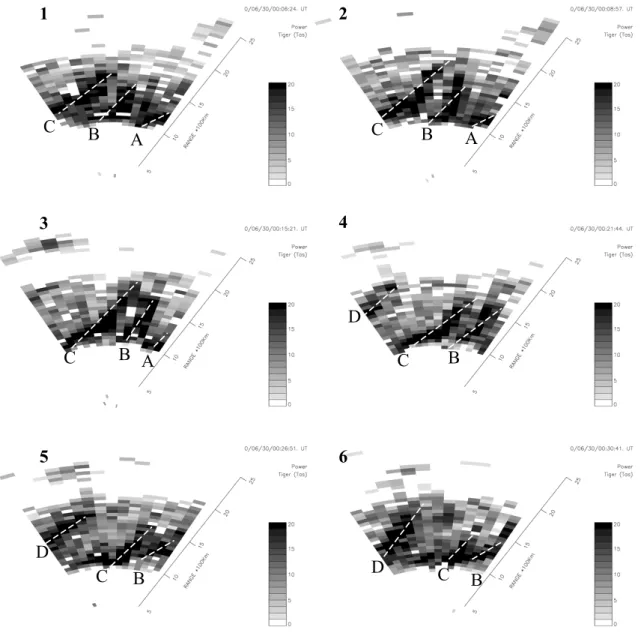
Fig. 3. A selection of TIGER full scans recorded during 00:06:24 to 00:30:41 UT on 30 June 2000. The parameter shown is sea echo power
in dB, and has not been band-pass filtered. Beam 0, the westernmost beam, is on the left, and the radar scans from east to west, i.e. from beam 14 to beam 0. Beam 15, the easternmost beam, was not used. The equatorward direction is downwards on the plot. The wavefronts formed by the stronger echoes are shown in solid lines. The propagation direction of waves can be clearly seen from the left top to the right-bottom, i.e. northeast.
4-h time period, sea echoes often occurred at many observa-tion cells, so this first stage of analysis generally produced many power spectra for further analysis.
For the next stage of analysis a cross spectral analysis method was developed to identify, for a given time window, the two-dimensional wave numbers of dominant MSTIDs ap-pearing within the full radar’s field of view.
Let k=(kx, ky)represent an AGW of wave number k
prop-agating across the TIGER’s field of view. The origin of the axis system is the TIGER site, i.e. at zero radar range, and the axis points to geographic north, so that the negative x-axis points to geographic south between radar beams 7 and 8. The y-axis is taken as positive east (see Fig. 1). In or-der to simplify the calculations, the MSTIDs were regarded
as isolated, single wave packets; calculations were carried out assuming each significant frequency in a power spectrum was an independent MSTID.
Figure 2 shows the flow chart of the FFT cross-spectral analysis method used to determine MSTID wave numbers from the observations. Consider a time window centered on time, τ , and a specific observation cell to be used as a refer-ence cell and denoted by (b, r), where b is the beam number and r is the range. The frequency spectrum of the associ-ated fluctuations observed by the radar in this reference cell,
Ab,r,τ (ω), can then be written as
4080 L.-S. He et al.: Studies of medium-scale travelling ionospheric disturbances
16
Fig. 3
Fig. 4
A
B
C
A
B
C
A
B
C
C
B
D
B
C
D
B
C
D
1
3
5
2
4
6
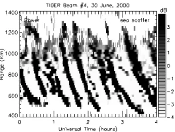
Fig. 4. Range-time-intensity plot of sea scatter power recorded from
00:00 UT to 04:00 UT on 30 June 2000 using TIGER beam 4. The time series of echo power were band-pass filtered over the period range 10 to 100 min. An HF propagation factor, r=0.5, was applied to the range.
where b=0, 2, 3, . . . bmax; r=1, 2, 3, . . . rmaxand bmax≤15, rmax≤75.
The corresponding cross-spectra φb,r,b0,r0,τ (ω) of
fluctua-tions occurring in the reference cell (b, r) and adjacent ob-servation cells (b0, r0) are given by:
φb,r,b0,r0,τ(ω)=φb,r,b0,r0,τ(ω)e−i(kx(xb,r−xb0,r0)+ky(yb,r−yb0,r0)) (2)
φb,r,b0,r0,τ(ω)=Ab,r,τ(ω)A∗b0,r0,τ(ω). (3)
In the analysis the difference between the phases (i.e. the cross phases given in Eq. (2) were calculated for all three-cell combinations of a reference cell and other cells. The orthog-onal distances between the center of the cells, 1x and 1y, were calculated using spherical trigonometry, to allow for the azimuthal spreading of the beams with increasing range. The meridian and zonal wave numbers were then obtained using
kx=1φx/1xand ky=1φy/1y. This analysis procedure
produced a spread in wave number values. Histograms show-ing the number of times particular wave numbers occurred were calculated and used to identify the meridional and zonal components of the dominant wave vectors. In practice, these calculations were performed at only a relatively few MSTID wave periods, viz. those given by spectral peaks that were greater than the mean level of spectral power at periods in the range 20 to 50 min.
In order to prevent spatial aliasing, a maximum range separation between cells was set for use in the three-cell analysis. Applying the wave-vector analysis to cells adja-cent in range (45 km) eliminated aliasing for wave numbers
|kx|>70×10−6m−1. The calculation of the aliasing for kyis
also affected by some other factors. If the effect of the HF propagation is taken by 0.5 (Bristow et al., 1994), at range gate 40 (i.e. 990 km for sea echoes) and 3.25◦between two beams, the spatial sampling is 56 km. Thus, the critical value of |ky| is 56×10−6m−1. These aliasing will not affect our
Table 1. Parameter comparison for periods of 60, 40, 26 and 20 min
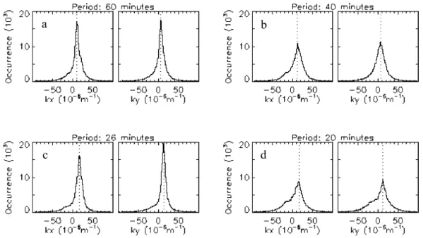
derived by FFT. Period (min) 60 40 26 20 kx(106m−1) 10 12 16 16 ky10−6 m−1) 5 6 13 12 Wavelength (km) 562 468.3 304.8 314.2 Speed (m s−1) 155.3 194.2 189.5 260.4 Azimuth (◦) 27 (NE) 27 (NE) 39 (NE) 37 (NE)
calculations on the wave vectors of MSTIDs, since the wave-lengths of MSTIDs were usually at the rages of 400–600 km (k is between 10–16×10−6m−1).
Finally, the determination of the MSTID wave period and orthogonal wave-vector components enabled the calculation of the following wave parameters:
(a) the phase velocity, using:
Vph=ω(kx2+k 2 y)
−1/2 (4)
(b) the wave propagation direction, using:
Az=tan−1(ky/ kx) (5)
(c) the wavelength, using:
λ=2π(k2x+ky2)−1/2. (6) Application of this cross-spectral analysis method pro-vided information on the two-dimensional dispersion of MSTIDs, so the spatial and temporal coherency of MSTIDs across the radar’s field of view could be investigated.
3 Case studies of MSTIDs observed on 29/30 June 2000
The day 30 June 2000 was the magnetically quietest day of this winter month, with Kp ranging between 0 and 2+ and
the AE index less than 200 nT. During this day, TIGER was operated in a discretionary mode (called “Basyouhup”), in which beams 5, 7 and 9 were set to a higher sampling rate for a ULF wave study and beam 15 was switched off. Therefore, these four beams were not used for the calculation of MSTID wave parameters.
Plots of TIGER full scans showing the sea echo power ob-served between 00:06–00:31 UT are presented in Fig. 3. Dur-ing this period, the sea echoes were concentrated between range gates 20 and 40 (i.e. at ranges of 1080 to 1980 km shown in Fig. 3). The wavefronts formed by the stronger echoes are marked by dashed lines. Beam 0, the western-most beam, is on the left, and beam 15 is on the right. The radar scans from east to west, i.e. from beam 14 to beam 0. At 00:06:24 UT (the scan labeled 1 in Fig. 3), three wave-fronts can be clearly seen. Wavefront A occurs across beams
L.-S. He et al.: Studies of medium-scale travelling ionospheric disturbances 4081
Fig. 5. Stack plot of power spectra calculated for range gates 20 to 40 along all beams, except beams 5, 7, 9 and 15. The scale for spectral
power is 2.5×10⁴count2mHz−1per range bin. The solid lines show the power levels at periods of 60, 40, 26 and 20 min from beam 4. They are well above the background noise level along most of these beams.
12 to 14, B across beams 5 to 9, and C across beams 0 to 7. By 00:08:57 UT (scan 2 in Fig. 3) there has been signifi-cant movement of wavefronts A, B and C towards the bottom right, i.e. to the northeast. By 00:21:44 UT (scan 4), wave-front A has moved out of the radar’s field of view (FOV) and a new wavefront, D, has appeared at the top left (south-east). Throughout the sequence wavefront C moves from the left (west) to the central region of the FOV. By 00:30:41 UT (scan 6), wavefront B has nearly disappeared from the FOV and D has continued to propagate to the right (east) and is a dominant feature on the left side of the FOV.
Figure 4 shows range-time plots of sea echo power observed along beam 4 from 00:00 to 04:00 UT on 30 June 2000, after band-pass filtering the data to display the effects of periods in the range 10 to 100 min. The choice of HF propagation factor used to rescale the data to give the
range to the ionospheric reflection point will be discussed later. MSTIDs are clearly evident in the form of sloping quasi-periodic power enhancements that move toward the radar (i.e. northward) with time. Figure 5 shows power spec-tra of the time series of echo power recorded during this pe-riod for all beams except beams 5, 7, 9 and 15, as previ-ously explained. Spectral peaks well above the background noise along beam 4 have periods of 20 min (frequency of 0.83 mHz), 26 min (0.62 mHz), 40 min (0.41 mHz), and 60 min (0.28 mHz) and these are marked by solid lines to aid comparison with Fig. 6. Along beams 10, 11, 12, 13 and 14 these waves are weaker and more dispersed. The waves with periods of 20 and 40 min are also weak in the directions of beams 0, 1, and 2.
The average power spectra of the fluctuations of sea scatter amplitude along all the ranges of (a) beam 4 and (b) beam 8
4082 L.-S. He et al.: Studies of medium-scale travelling ionospheric disturbances Fig. 5. Continued.
18
Fig. 5
Fig. 6
a
b
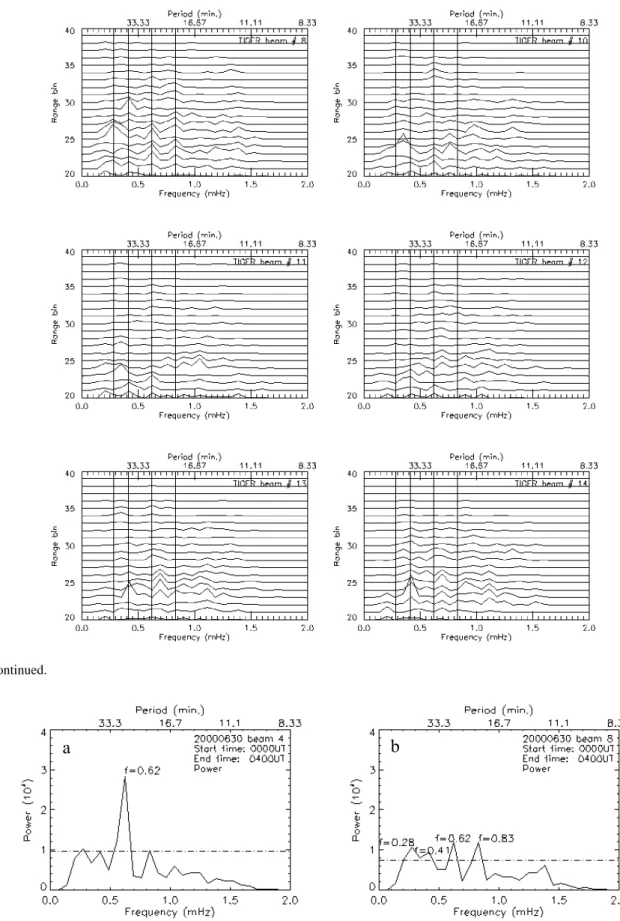
Fig. 6. The averaged power spectra of the fluctuations of sea scatter powers during the interval of 00:00 UT to 04:00 UT, on 30 June 2000
along beam 4 (a) and beam 8 (b). The dotted line indicates the mean power level of the TIDs’ significant frequencies from 0.83 mHz (20 min) to 0.33 mHz (50 min).
L.-S. He et al.: Studies of medium-scale travelling ionospheric disturbances 4083
19
Fig. 7 a-d
Fig. 8
a
b
c d
Fig. 7. Distributions of gravity wave number vector at periods of 60 (a), 40 (b), 26 (c) and 20 (d) min, respectively. The maxima of the
distributions are used to estimate the wave wavelengths, phase velocities and azimuthal angles of propagation.
during the interval 00:00 UT to 04:00 UT, on 30 June 2000, are shown in Fig. 6. TIGER beam 4 looks towards the ge-omagnetic pole and beam 8 looks almost directly towards the geographic pole. The broken line in Fig. 6 indicates the mean power level over the frequency range from 0.83 mHz (20 min) to 0.33 mHz (50 min). The mean power level was used as an arbitrary measure of background wave activity. Only the peaks above the mean power level were regarded as significant. For beam 4, the only significant spectral peak is at 0.62 mHz. For beam 8, significant peaks occur at four frequencies.
As described in Sect. 2 the phase velocity and azimuth of the MSTIDs were estimated by calculating phase dif-ferences using combinations of three observation cells for which nearly continuous sea echoes were recorded through-out the chosen four-hour time window. As already explained, only combinations of adjacent observation cells were used to limit the effects of spatial aliasing in the kx and ky
direc-tions. The spatial ranges along kxand ky directions are
sim-ply taken as less than 300 km. The results, when plotted as a histogram, identify the most coherent waves moving across the array.
Figures 7a–d show histograms of the two orthogonal com-ponents of the horizontal wave numbers (kx and ky)
de-rived in this manner at the four different periods iden-tified in the data. For the 20.0-min period (0.83 mHz) shown in (a), the maxima in the distributions of kx and
ky were at 16.0×10⁻⁶m−1 and 12.0×10⁻⁶m−1,
respec-tively. Hence, using Eqs. (4), (5) and (6), the apparent phase velocity of the dominant wave component was found to be 260 m s−1, the apparent wavelength was 314.20 km, and the azimuth angle was 36.90◦ (i.e. close to NE). For the 26.0-min period (0.62 mHz) shown in (b), the maxima
19
Fig. 7 a-d
Fig. 8
a
b
c d
Fig. 8. Comparison of TID observational (dash-line arrow) and
cal-culated (solid-line arrow) propagation. The slopes of solid lines are given by wavefront “C” shown in Fig. 3. The numbers correspond to the time series in Fig. 3.
in the distributions of kx and ky were at 16.0×10⁻⁶m−1
and 13.0×10⁻⁶m−1, respectively. Hence, the apparent
phase velocity was 189.5 m s−1, the apparent wavelength was 304.80 km, and the azimuthal angle was 39.10◦. For the 40.0-min period (0.41 mHz) shown in (c), maxima in the distributions of kx and ky occurred at 12.0×10⁻⁶m−1
and 6.0×10⁻⁶m−1, respectively. Hence, the apparent phase velocity was 194.1 m s−1, the apparent wavelength was 468.3 km, and the azimuthal angle was 26.60◦. For the 60.0-min period (0.28 mHz) shown in (d), the maxima in the distributions of kx and ky were at 10.0×10⁻⁶m−1 and
4084 L.-S. He et al.: Studies of medium-scale travelling ionospheric disturbances
20
Fig. 9
Fig. 10
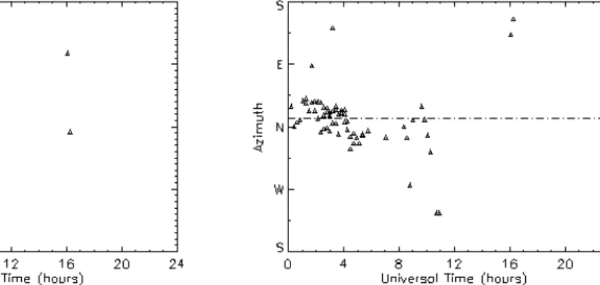
Fig. 9. The diurnal variation of speed (left) and azimuth (right) on 30 June 2000. The reference beam is beam 4. The dot-dashed line
indicates geomagnetic north.
20
Fig. 9
Fig. 10
Fig. 10. Same as Fig. 9, except the reference beam is chosen along beam 13.
5.0×10⁻⁶m−1, respectively. Hence, the apparent phase velocity was 155.3 m s−1, the apparent wavelength was 562.0 km, and the azimuthal angle was 26.60◦(see Table 1). Figure 8 shows the comparison of the direction for wave C calculated using the FFT method and determined directly from Fig. 3. The latter method is less accurate, but there is good agreement between the value of ∼39◦ determined by the full analysis and the value of ∼43◦E of N estimated di-rectly from the full-scan plots. In many instances MSTID wavefronts are not so readily identified in full-scan data, hence the development of the FFT method.
Significant peaks in the power spectra do not always oc-cur at precisely the same periods along all beams, so a spe-cific beam is chosen as a reference beam. Figure 9 shows the diurnal variation of MSTID speed and azimuth with time using beam 4 as the reference beam on 30 June 2000. The sea echoes appear between 00:00–10:00 UT and 16:00– 20:00 UT. The analysis was not extended beyond 20:00 UT because the 4-h time window would then extend into 1 July, when it so happened that a different data sampling rate was used which would complicate the FFT analysis. The analysis method described above was used to determine the behavior of the dominant wave number at each frequency identified by the mode values, i.e. the peaks in the wave number dis-tributions. It is evident that the MSTID phase speeds were
mainly between 100–300 ms−1. The azimuth plot indicates propagation primarily towards the northeast before 04:30 UT (i.e. 14:30 LT) and then a change to primarily the northwest direction. During 16:00–20:00 UT (i.e. 02:00–06:00 LT), the MSTID propagation direction became quite variable, with both the north and southwest directions predominant.
In order to test the consistency of the analysis technique, beam 13 was chosen as the reference beam and the results compared with those obtained using beam 4 as the refer-ence beam. Figure 10 shows the phase speed and azimuth. Compared to the results obtain using beam 4, the phase speeds are also around 200 ms−1. The propagation direction also changed from being northeast to northwest at around 04:00 UT, nearly half an hour earlier than the result obtained using beam 4. After 16:00 UT very few waves were detected along beam 13.
4 Characteristics of MSTID propagation characteris-tics derived from sea echoes
The FFT and cross-spectral methods were used to deter-mine the propagation directions using TIGER observations throughout the year 2000. Typically 14 to 20 days of suitable observations (primarily common mode) were obtained in
L.-S. He et al.: Studies of medium-scale travelling ionospheric disturbances 4085
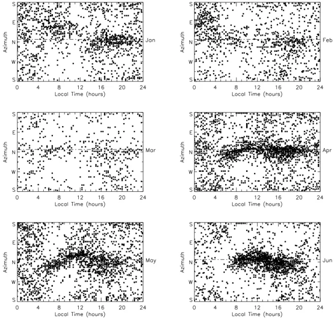
Fig. 11. Diurnal variation of MSTID propagation determined using sea scatter from January to December 2000. The dashed line indicates
magnetic north.
each month. The smallest monthly numbers of observing days occurred in March and August which had only 8 and 9 days, respectively. The maximum number occurred in October when there were 30 days of observations. In order to provide a more meaningful description, the results are now presented in terms of LT rather that UT.
Figure 11 shows diurnal variations of MSTID propaga-tion direcpropaga-tion obtained using sea scatter echoes recorded us-ing beam 4 as the reference beam. Again, dominant spec-tral peaks have been identified as those greater than the mean power level over the MSTID period range of 20 min to 50 min typically observed by SuperDARN radars (e.g. Bristow et al., 1994).
The plots can be divided into four sectors, viz. early morn-ing, pre-noon, afternoon and evening. In the early mornmorn-ing, the propagation directions are quite variable. In the pre-noon and the afternoon, the propagation was mainly toward the north (i.e. equatorward) during spring and summer (i.e. from September to February). Fewer MSTID events occurred at noon in these seasons. There were clearly preferred propaga-tion direcpropaga-tions from April to July, particularly during the day with MSTIDs propagating predominantly to the northwest at the beginning of the day, and then changing to the north-east at ∼09:00 LT. In the afternoon and evening sectors, the propagation generally changed back to the north/northwest at ∼14:00 LT.
4086 L.-S. He et al.: Studies of medium-scale travelling ionospheric disturbances
Fig. 11. Continued.
5 Discussion
The technique using the Fourier transform and cross-spectral analyses has been developed for use with SuperDARN sea echo data to identify the properties of MSTIDs. In this method, we used the mode values, i.e. the peaks in the distri-butions to identify the dominant wave numbers at each fre-quency.
Earlier it was indicated that time series could be included in the analysis even when the time series of sea echoes did not extend throughout an entire 4-h time window; however, this was done only if sea echo data existed over at least 70% of the window length. If under this criterion, over 90% of cells along a beam were unsuitable for analysis, the beam was removed from the analysis.
Figure 3 clearly shows the propagation of dominant wave components. The directions estimated from this figure are also consistent with the directions determined by the anal-ysis method (Fig. 8). From the power spectrum analy-sis, we found that the frequencies obtained by FFT along some beams were different from other beams. However, the MSTID phase speeds and propagation directions were not very different when determined using different beams as the reference beam, because there was little variation in the wave number values determined from the histograms.
In the phase speed calculations, the effect of the HF prop-agation factor, r, must be considered. We favored the use of the simplest value, i.e. r=1/2 for sea scatter, and this factor was used by Bristow et al. (1994) after they com-pared the AGW features using Goose Bay SuperDARN radar
L.-S. He et al.: Studies of medium-scale travelling ionospheric disturbances 4087 observation with the theoretical wave phase surface. Others
have suggested that a larger value of r should be used 0.6 (Hall et al., 1999) or 1.0 (MacDougall et al., 2000). However, as TIGER is at a lower latitude than other radars and further from the sources generating the MSTIDs, the effect of the MSTIDs on the background ionosphere is likely to be less and this will favour using r=0.5. Furthermore, here we are interested primarily in the directions of propagation rather than the actual range to the ionospheric reflection points and determination of the propagation direction is not greatly af-fected by the choice of r.
From the study, we found that the propagation direction in early morning and late evening was quite variable but was clearly equatorward during the daytime (Fig. 11). At noon fewer MSTID events were observed in summer, spring and early autumn. But in later autumn and winter, the prop-agation direction showed a significant change from north-west to northeast at around 09:00 LT in the pre-noon, and from northeast to northwest at around 14:00 LT in the after-noon. Northeast propagation on the dayside is also consis-tent with that found by Munro (1958) and Scali (1989). The significant statistical studies by Munro indicated that day-time MSTIDs travelled toward the northeast in the Southern Hemisphere winter. Scali also obtained similar results when investigating MSTIDs causing spread F at the mid-latitude station, Beveridge (145.1◦S, 37.8◦E, Geographic), which is several hundred kilometers equatorward of the TIGER radar site in Tasmania. The northwest propagation direction in the evening is also consistent with some previous studies (e.g. Bowman, 1960; From and Meehan, 1988).
It is also likely that the dayside MSTIDs are caused by the Lorenz force, which can be written as:
L =j⊥×B = (σpE − σHE × B/B) × B
=σpE × B + σHEB .
Here, σH>σP, where σH is the Hall conductivity and σP is
the Pedersen conductivity. Thus, both transition propagation direction at 09:00 and 14:00 LT on the dayside are generally consistent with the variations of ionospheric electric fields (Friis-Christensen et al., 1985), but in the early morning sec-tor the electric fields change their directions around 05:00 LT and MSTID propagation directions changed at 09:00 LT. This is because the propagation directions are also affected by the Pedersen current term in the Lorentz force term (i.e.
σpE×B). The time delay is probably also because the
elec-tric field directions were derived from magnetometer obser-vations in summer and MSTID propagation directions signif-icantly change in winter.
At noon, few MSTIDs events were observed in most sea-sons. It may be caused by the ion-drag effects in the day-time ionosphere which may reduce the observed TID activity (e.g. Balthazor and Moffett, 1999). The variable propagation directions in the early morning are likely caused by the ir-regular magnetic disturbance regions discussed by Iijima et al. (1978), who found a highly structured magnetic distur-bance region existing in the morning sector during the
sub-storm recovery phase; some structure even exists during ge-omagnetically quiet conditions.
6 Conclusions
A technique using FFT and cross-spectral analysis has been developed and applied to TIGER HF radar observations to determine propagation characteristics of medium-scale trav-elling ionospheric disturbances. A case study showed that the method clearly identifies dominant MSTIDs propagating through radar field of view.
Statistical studies using sea echoes show that the propaga-tion direcpropaga-tions have a strong local time dependency through-out all seasons. In the early morning the propagation di-rections are irregular. Near dawn and dusk, there is pro-nounced equatorward propagation. At noon there are rela-tively few MSTID events in summer, spring and early au-tumn. In later autumn and winter, propagation at noon is primarily northeast, after changing from northwest at around 09:00 LT. At around 14:00 LT the direction changes back to north/northwest. It is suggested that the irregular propagation in the morning is related to the field-aligned current irregu-lar disturbance region and the Lorentz force is the possible cause of the dayside MSTID excitation.
Acknowledgements. The comments from P. Wilkinson of Aus-tralian IPS and K. D. Cole of La Trobe University are acknowl-edged. The work is supported by the Australian Research Coun-cil, the organizations constituting the TIGER consortium. LSH also acknowledged the supports from the Australian International Postgraduate Research Scholarship Scheme and the La Trobe Uni-versity Postgraduate Scholarship Scheme.
Topical Editor M. Lester thanks a referee for his/her help in evaluating this paper.
References
Balthazor, R. L. and Moffett, R. J.: Morphology of large-scale traveling atmospheric disturbances in the polar thermosphere, J. Geophys., Res., 104, 15–24, 1999.
Bowman, G. G.: Further studies of spread F at Brisbane I, Planet. Space Sci., 2, 133–149, 1960.
Brekke, A.: On the relative importance of Joule heating and the Lorentz force in generating atmospheric gravity waves and infra-sound waves in the auroral electrojets, J. Atmos. Terr. Phys., 41, 475–479, 1979.
Briggs, B. H.: On the analysis of moving patterns in Geophysics-1: Correlation analysis, J. Atmos. Terr. Phys., 30, 1777–1788, 1968a.
Briggs, B. H.: On the analysis of moving patterns in Geophysics-2: Dispersion analysis, J. Atmos. Terr. Phys., 30, 1789–1794, 1968b.
Bristow, W. A., Greenwald, R. A., and Samson, J. C.: Identification of high-latitude acoustic gravity sources using the Goose Bay HF radar, J. Geophys., Res., 99, 319–331, 1994.
Bristow, W. A. and Greenwald, R. A.: Estimating gravity wave parameters from oblique high-frequency backscatter: Modeling and analysis, J. Geophys. Res., 100, 3639–3648, 1995.
4088 L.-S. He et al.: Studies of medium-scale travelling ionospheric disturbances
Bristow, W. A., Greenwald, R. A., and Villain, J. P.: On the seasonal dependence of medium-scale atmospheric gravity waves in the upper atmosphere at the high latitudes, J. Geophys. Res., 101, 15 685–15 700, 1996.
Bristow, W. A. and Greenwald, R. A.: On the spectrum of thermo-spheric gravity waves observed by the Super Dual Auroral Radar Network, J. Geophys. Res., 102, 11 585–11 596, 1997.
Chimonas, G. and Hines, C. O.: Atmospheric Gravity waves launched by auroral currents, Planet Space Sci., 18, 565–582, 1970.
Crowley, G., Jones, T. B., and Dudeney, J. R.: Comparison of short period TID morphologies in Antarctica during geomagnetically quiet and active intervals, J. Atmos. Terr. Phys., 49, 1155–1162, 1987.
Dyson, P. L. and Devlin, J. C.: The Tasman International Geospace Environment Radar, The Physicist (The Australian Institute of Physics), 37, 48–53, 2000.
Francis, S. H.: A theory of medium-scale traveling ionospheric dis-turbances, J. Geophys. Res., 79, 5245–5260, 1974.
Francis, S. H.: Global propagation of atmospheric gravity waves: a review, J. Atmos. Terr. Phys., 37, 1011–1054, 1975.
Friis-Christensen, E., Kamide, Y., Richmond, A. D., and Mat-sushita, S.: Interplanetary magnetic field control of high-latitude electric fields and currents determined from Greenland magne-tometer data, J. Geophy. Res., 90, 1325–1338, 1985.
From, W. R. and Meehan, D. H.: Mid-latitude spread F structure, J. Atmos. Terr. Phys., 50, 629–638, 1988.
Hall, G. E., MacDougall, J. W., Cecile, J.-W., Moorcroft, D. R., and St. Maurice, J. P.: Finding gravity wave source positions using the Super Dual Auroral Radar Network, J. Geophys. Res., 104, 67–78, 1999.
Huang, C.-S., Dieter, A. A., and Sofko, G. J.: High-latitude iono-spheric perturbations and gravity waves: 1. Observational re-sults, J. Geophys. Res., 103, 2131–2142, 1998a.
Huang, C.-S., Dieter, A. A., and Sofko, G. J.: Observations of so-lar wind directly driven auroral electrojets and gravity waves, J. Geophys. Res., 103, 23 346–23 356, 1998b.
Hunsucker, R. D.: Estimate of relative importance of Joule heating and Lorenta force in generating atmospheric gravity waves from the auroral electrojet, J. Geophy. Res., 82, 4826–4828, 1977. Iijima, T. and Potemra, T. A.: Large-scale characteristics of
field-aligned currents associated with substorms, J. Geophys. Res., 83, 599–615, 1978.
Jing, N. and Hunsucker, R. D.: A theoretical investigation of sources of large and medium scale atmospheric gravity waves in the auroral oval, J. Atmos. Terr. Phys. 55, 1667–1679, 1993. MacDougall, J. W., Andre, D. A., Sofko, G. J., Hunag, C.-S., and
Koustov, A. V.: Travelling ionospheric disturbance properties de-duced from Super Dual Auroral Radar measurements, Ann. Geo-phys., 18, 1550–1559, 2000.
Munro, G. H.: Travelling ionospheric disturbances in the F-region, Aust. J. Phys., 29, 91–112, 1958.
Ogawa, T., Igarashi, K., Aikyo, K., and Maeno, H.: NNSS satel-lite observations of medium-scale travelling ionospheric distur-bances at southern high latitudes, J. Geomagn. Geoelectr., 39, 709–721, 1987.
Richmond, A. D.: Gravity wave generation, propagation, and dis-sipation in the thermosphere, J. Geophys. Res., 83, 4131–4145, 1978.
Samson, J. C., Greenwald, R. A., Ruohoniemi, J. M., and Baker, K. B.: High-frequency radar observations of atmospheric gravity waves in the high-latitude ionosphere, Geophys. Res. Lett., 16, 875–878, 1989.
Samson, J. C., Greenwald, R. A., Ruohoniemi, J. M., Frey, A., and Baker, K. B.: Goose Bay radar observations of Earth-reflected at-mospheric gravity waves in the high-latitude ionosphere, J. Geo-phys. Res., 95, 7693–7709, 1990.
Scali, J. L.: A study of spread-F irregularities at mid-latitudes, Ph.D thesis, La Trobe University, 1989.
Shibata, T.: Application of multichannel maximum entropy spec-tral analysis to the HF Doppler Data of medium-scale TID, J. Geomagn. Geoelectr., 39, 247–260, 1987.
Sofko, G. and Huang, C.-S.: SuperDARN observations of medium-scale gravity wave pairs gnereated by Joule Heating in the auroral zone, Geophys. Res. Lett., 27, 485–488, 2000.
Tsutsui, M., Horikawa, T., and Ogawa, T.: Determination of ve-locity vectors of thermospheric wind from dispersion relation of TID’s observation by an HF Doppler array, J. Atmos. Terr. Phys., 46, 447–462, 1984.
Wan, W. X., Yuan, H., and Liang, J.: An analysis method of non-uniform ionospheric disturbances from array observation, Chi-nese J. Geophys., 39, 183–190, 1996.