Probability distribution of flood flows in Tunisia

(1)

HAL Id: hal-00298830

https://hal.archives-ouvertes.fr/hal-00298830

Submitted on 27 Apr 2007

HAL is a multi-disciplinary open access

archive for the deposit and dissemination of sci-entific research documents, whether they are pub-lished or not. The documents may come from teaching and research institutions in France or abroad, or from public or private research centers.

L’archive ouverte pluridisciplinaire HAL, est destinée au dépôt et à la diffusion de documents scientifiques de niveau recherche, publiés ou non, émanant des établissements d’enseignement et de recherche français ou étrangers, des laboratoires publics ou privés.

Probability distribution of flood flows in Tunisia

H. Abida, M. Ellouze

To cite this version:

H. Abida, M. Ellouze. Probability distribution of flood flows in Tunisia. Hydrology and Earth System Sciences Discussions, European Geosciences Union, 2007, 4 (2), pp.957-981. �hal-00298830�

(2)

HESSD

4, 957–981, 2007

Probability distribution of flood

flows in Tunisia H. Abida and M. Ellouze

Title Page Abstract Introduction Conclusions References Tables Figures ◭ ◮ ◭ ◮ Back Close

Full Screen / Esc

Printer-friendly Version Interactive Discussion

EGU

Hydrol. Earth Syst. Sci. Discuss., 4, 957–981, 2007 www.hydrol-earth-syst-sci-discuss.net/4/957/2007/ © Author(s) 2007. This work is licensed

under a Creative Commons License.

Hydrology and Earth System Sciences Discussions

Papers published in Hydrology and Earth System Sciences Discussions are under open-access review for the journal Hydrology and Earth System Sciences

Probability distribution of flood flows in

Tunisia

H. Abida1and M. Ellouze2

1

Department of Earth Sciences, Faculty of Science, Sfax, BP 802, 3018, Tunisia

2

Faculty of Science of Sfax, Sfax, Tunisia

Received: 16 February 2007 – Accepted: 1 March 2007 – Published: 27 April 2007 Correspondence to: H. Abida (habib.abida@voila.fr)

(3)

HESSD

4, 957–981, 2007

Full Screen / Esc

EGU

Abstract

L (Linear) moments are used in identifying regional flood frequency distributions for different zones Tunisia wide. 893 site-years of annual maximum stream flow data from a total of 37 stations with an average record length of 24.14 years are considered. The country is divided into two homogeneous regions (northern and central/southern

5

Tunisia) using a heterogeneity measure, based on the spread of the sample L-moments among the sites in a given region. Then, selection of the corresponding distribution is achieved through goodness-of-fit comparisons in L-moment diagrams and verified us-ing an L-moment based regional test that compares observed to theoretical values of L-skewness and L-kurtosis for various candidate distributions. The distributions used,

10

which represent five of the most frequently used distributions in the analysis of hydro-logic extreme variables are: (i) Generalized Extreme Value (GEV), (ii) Pearson Type III (P3), (iii) Generalized Logistic (GLO), (iv) Generalized Normal (GN), and (v) Gener-alized Pareto (GPA) distributions. Spatial trends, with respect to the best-fit flood fre-quency distribution, are distinguished: Northern Tunisia was shown to be represented

15

by the GEV distribution while the GLO distribution gives the best fit in central/southern Tunisia.

1 Introduction

Peak or flood flow is an important hydrologic parameter in the determination of flood risk, management of water resources and design of hydraulic structures such as dams,

20

spillways, culverts and irrigation ditches. The estimate of the design event must be fairly accurate to avoid excessive costs in the case of overestimation of the flood mag-nitude or excessive damage and even loss of human lives while underestimating the flood potential. There is a need, therefore, to estimate how often a specific flood event will occur, or how large a flood will be for a particular probability of exceedence or

25

(4)

proce-HESSD

4, 957–981, 2007

Full Screen / Esc

EGU

dures, which involve the estimation of distributional parameters and the extrapolation of cumulative distribution functions to generate extreme flood values.

Flood frequency analysis is performed either for a single site, when extensive historic peak flow data are available, or on a regional basis, when there is little or no historic flow data at a particular site. In this latter case, all data from other local basins within

5

the same region are pooled to get an efficient estimate of parameters of a chosen distribution and hence a more robust quantile estimate. Bobee and Rasmussen (1995) reported that the use of regional information allows a reduction of sampling uncertainty by introducing more data, as well as a reduction of model uncertainty by facilitating a better choice of distribution.

10

Recently, research efforts focused more on regional rather than the conventional at-site flood frequency analysis. Hosking and Wallis (1993) organized regional flood frequency analysis into 4 stages: (i) screening of the data, (ii) identification of homo-geneous regions, (iii) choice of a regional probability distribution, and (iv) estimation of the regional flood frequency distribution. Recent research efforts also focused on

15

the use of L-moment diagrams for the identification of flood frequency distributions, such as the studies performed in Bangladesh (Abdul karim and Chowdhury, 1995), New Zealand (Pearson, 1991), Australia (Nathan and Weinmann, 1991), Canada (Pi-lon and Adamowski, 1992; Nguyen, 2006), United States (Wallis, 1988; Vogel and Wilson, 1996), China (Jingyi and Hall, 2004), India (Rakesh and Chandranath, 2006)

20

and the globe (Onoz and Bayazit, 1995). In fact, there appear to be a general world-wide agreement among agencies and governments to re-evaluate their flood frequency standard procedures using L-moment based techniques.

In this context, this study uses L-moment diagrams to select the flood frequency distribution that best fits the annual maximum flood flows in Tunisia. The paper first

25

presents a survey of similar previous L-moment-based studies all over the world. Then, the study area and the data used in the numerical analysis are described. Next, the flood frequency identification procedure is presented. Finally, the results of the analysis are discussed and summarized.

(5)

HESSD

4, 957–981, 2007

Full Screen / Esc

EGU

2 Literature review

2.1 Global survey of flood frequency models

Many statistical distributions for flood-frequency analysis have been investigated in hy-drology. Annual flood series were found to be often skewed, which led to the de-velopment and use of many skewed distributions, with the most commonly applied

5

distributions now being the Gumbel (EV1), the Generalized Extreme Value (GEV), the Log Pearson Type III (LP3), and the 3 parameter Lognormal (LN3) (Pilon and Harvey, 1994). The proponents of each distribution have been able to show some degree of confirmation for their particular distribution by comparing theoretical results and mea-sured values. However, there is no theoretical basis for justifying the use of one specific

10

distribution for modeling flood data and long term flood records show no justification for the adoption of a single type of distribution (Benson, 1968).

Different studies were undertaken on distribution selection for flood data in different countries all over the world. Beard (1974) estimated the 1000 year floods at 300 sta-tions in USA with 14200 station-years of data by eight different models and concluded,

15

based on split sample experiments, that the two parameter lognormal (LN2) and the log Pearson Type III (LP3) were the best. Gunasekara and Cunnane (1992) repeated the split sample experiments of Beard (1974) with synthetic data consisting of samples of 40 events. They concluded that the GEV distribution with probability weighted mo-ments (PWMs) estimated parameters was the best at-site method to estimate the 100

20

and 1000 year floods and the LP3 with regional skew yielded comparable results. McMahon and Srikanthan (1981) used the moment ratio diagrams to compare var-ious distributions with the data from 172 streams in Australia and concluded that LP3 was the only one suitable. Farquharson et al. (1987) fit a GEV distribution to an-nual flood flow data at 1121 gauging stations in 70 different countries using probability

25

weighted moments. McMahon et al. (1992) and Finlayson and McMahon (1992) ana-lyzed annual maximum flood flow data at 974 stations around the world using ordinary product moment diagrams. The authors tested several probability distributions and

(6)

HESSD

4, 957–981, 2007

Full Screen / Esc

EGU

concluded that the LP3 distribution provided the best fit to observed flood flow data. However, other testing methods should have been used in this study because the estimates of ordinary product moment ratios such as the coefficient of variation and skewness contain significant bias (Vogel and Fennessey, 1993), especially for small and highly skewed samples.

5

2.2 Standard distributions adopted by National Institutions in the World

Based on large scale studies of their own flood data, many countries adopted standard methods to be used by governments or private agencies to achieve uniformity in flood frequency analysis and estimation. A working group in the USA (US Water Resources Council (Benson, 1968) recommended the LP3 distribution whereas a similar study in

10

the United Kingdom (NERC, 1975) proposed the GEV distribution as a standard. The generalized gamma distribution was recommended in the former USSR (Kritsky and Menkel, 1969) while the P3 and the LP3 distributions were generally recommended in West Germany. The LP3 distribution was also advocated by the Institution of Engineers in Australia (Institution of Engineers, Australia (IEA, 1977).

15

More recently, a worldwide survey of flood frequency methods, prepared for the World Meteorological Organization in 1984 and involving 55 agencies from 28 coun-tries, reported the use of six distributions namely EV1, EV2, GEV, LN2, P3, and LP3. The survey, which was summarized by Cunnane Cunnane (1989), revealed that EV1, LN2, P3, and LP3 were the most common distributions while only one country used

20

the GEV distribution in spite of its recent popularity.

2.3 L-moments and flood frequency analysis

In the last century, probably one of the most significant scientific contributions to statis-tical hydrology is the L-moments of Hosking (1990). The advantages of the L-moments are that (i) they characterize a wider range of distributions than conventional moments,

25

(7)

HESSD

4, 957–981, 2007

Full Screen / Esc

EGU

normal distribution more closely, and (iv) they are nearly unbiased for all combinations of sample sizes and populations (Hosking and Wallis, 1990).

Wallis (1988), Cunnane (1989) and Hosking (1990) illustrated that, compared to the product moment ratio diagram, the L-moment ratio diagrams possess a better ability to discriminate between distributions. Vogel and Fennessey (1993) reported that

con-5

ventional product moment estimators should be replaced by L-moment estimators for most goodness-of-fit applications in hydrology. They showed that L-moment diagrams perform always better than ordinary product moment diagrams, regardless of the sam-ple sizes, probability distributions, or skews involved. Cong et al. (1993) reported that L-moment of-fit tests are more robust than classical single-site

goodness-10

of-fit tests since they use regional rather than single-site data to discriminate between alternative distributions.

Numerous studies have used L-moment diagrams in regional flood frequency analy-sis, most of which are summarized in Table 1. In spite of this recent tendency of using L-moments world-wide, Klemes (2000a, b) articulated some cautionary notes about

15

their use in hydrological frequency analysis. He claimed that L-moments artificially impose a structure upon a data set and de-emphasize the importance of observed ex-tremes, which leads to the underestimation of extreme design events. However, Alila and Mtiraoui (2002) argued that if the annual floods in a sample are distributed identi-cally and the outliers are caused by sampling variability (for instance, a 100-year event

20

in a 10-year sample) they should not be given an undue weight. If any historic informa-tion can be found for any high outlier, a reasonably well-established method, referred to as flood frequency analysis with historic information, could be used (Pilon and Harvey, 1994). Unfortunately, however, in the absence of any historic information, such high outliers are often either removed from the sample or simply ignored and, consequently,

25

the use of conventional moments would either over- or underestimates the T-year flood event. Therefore, in this case, it is more rational to use a method that is less sensitive to outliers in the data, such as L-moments.

(8)

mo-HESSD

4, 957–981, 2007

Full Screen / Esc

EGU

ments in using flood frequency analysis for the estimation of flood quantiles. This is particularly true when considering regional trends in higher order moment statistics. The use of L-moments permits the delineation of regional trends that otherwise might be obscured by biases and sampling variability [variability (Cathcart, 2001).

3 Study area

5

Tunisia is a relatively small (162 155 km2) North African country, located at the north-eastern tip of Africa at the center of the Mediterranean Sea. Linked on the west to the rest of North Africa by the mighty ridges of the Atlas Mountains, it stretches out to the south into the Sahara, of which it occupies a small part.

Opening on its northern and eastern fronts to the Mediterranean Sea, Tunisia enjoys

10

a clement and mild although notoriously capricious climate. By its latitude it is situated halfway between the temperate zone and the tropical zone, forming thus a meeting place at which cold air masses are confronted by the masses of warm air coming from the tropical regions. It has a rather unstable climate. When it is swept at the equinoxes by tides of opposing depressions, the result is severe cold fronts along with violent

15

storms and frequent downpours. With a general profile stretching lengthwise from north to south, Tunisia shows some climatic variations accentuated by its diversified geographical aspect. The Atlas Mountains stretching from east to west create a variety of large climatic areas distinct from each other mainly by their rainfall.

Rainfall in Tunisia might be crudely characterized by its shortage, irregularity and

20

erratic distribution, all leading either to periods of drought or intensive rainy periods, with storms causing disastrous flooding. The North receives an adequate and fairly reliable rainfall of approximately 600 mm. The central area has an annual mean of 200 mm, whilst the south receives less than 100 mm of rainfall. These averages are subject to very wide annual fluctuations of 1 to 6 for central Tunisia and 1 to 12 for the

25

South.

(9)

HESSD

4, 957–981, 2007

Full Screen / Esc

EGU

(Fig. 1):

– The High Tell or Northern Tunisia, characterized by its fertile soil and its high

degree of moisture. It is an area of high mountains surrounding plains irrigated by the Medjerda River and its tributaries. The western Tell is continued by the northeastern Tell, a maritime area on account of its being deeply penetrated by

5

the Gulf of Tunis and its climatic influences. This is an area of plains and hills crossed by large rivers such as the Medjerda and some of its tributaries and the Oued Miliane.

– Central Tunisia is the region that covers the high and low steppes stretching out

to the eastern coast. The high steppes represent a region of lofty mountains and

10

wide hollow dips, cut across by large creeks (wadis). The vegetation is made up of forests, often stunted, and fields of alfalfa grass. The continental climate contributes to the barrenness of the region. Further to the east the low steppe stretches over wide alluvial plains and hills cut across by large creeks running down the Atlas Mountains.

15

– Southern Tunisia, bordered on the west by Algeria and on the east by Libya, is

jutting out into the Sahara, of which it occupies a part.

4 Data used

A total of 49 annual flood series representing natural hydrologic regimes, obtained from the publications of the Tunisian Ministry of Agriculture and Water Resources, were used

20

for the identification of the appropriate flood frequency distribution.

Discharges were estimated by observing water levels and employing pre-calibrated rating curves to convert measured stages to observed flow rates. Rating curves were determined through velocity measurements using a current meter and graphic inte-gration of the velocity distribution over the entire cross-section. Regulated stations,

25

(10)

HESSD

4, 957–981, 2007

Full Screen / Esc

EGU

The annual flood data series need to be independent, random, homogeneous, and without trends. These properties were verified by four nonparametric tests using the Consolidated Frequency Analysis (CFA) package of Environment Canada (Pilon and Harvey, 1994).

Only 37 gauged stations met the screening criteria of having a minimum record

5

length of 10 years, representing unregulated natural flow regimes, and passing all of the nonparametric tests at the 5% level of significance.

5 Procedure used to select a distribution

The study area was divided arbitrarily into 3 sub-regions, for which separate flood frequency analysis procedures were performed. The procedure adopted to select

ap-10

propriate flood frequency distributions, first, uses the three statistical measures for regional flood frequency analysis of Hosking and Wallis (1993): (i) a discordance mea-sure for identifying unusual sites in a region, (ii) a heterogeneity meamea-sure, for assess-ing whether a proposed region is homogeneous, and (iii) a goodness of fit measure, for assessing whether a given distribution provides an adequate fit to the regional

15

annual maximum flood flow data. Then, flood frequency distributions are selected from L-moment diagrams that compare observed to theoretical values of L-skewness and L-kurtosis for various candidate distributions. In the selection process, either the weighted sample average or the line of best fit through the data points is used in the comparison with theoretical curves, depending on the outcome of the hetetrogeneity

20

test, as was recommended by Peel et al. (2001). 5.1 Discordance and heterogeneity tests

First, data screening was performed using the discordance measure of Hosking and Wallis (1993) to eliminate gross errors and inconsistencies. For each flood series, sites with Di>3, believed to be grossly discordant with the group as a whole, were dropped.

(11)

HESSD

4, 957–981, 2007

Full Screen / Esc

EGU

This resulted in decreasing the stations’ number from 37 to 31. Homogeneity test-ing was performed then, through the heterogeneity measure H, which is based on the spread of the sample L-moments among the sites in a given region. This statistic basi-cally compares the between-site variations in sample L moments for the group of sites with what would be expected for a homogeneous region. Hosking and Wallis (1993)

5

suggested that the region under testing should be regarded as “acceptably” homoge-neous if H<1, “possibly” heterogehomoge-neous if 1<H<2, and “definitely” heterogehomoge-neous if H>2.

Homogeneity was investigated only with respect to skewness and kurtosis because these dimensionless statistical characteristics are commonly used to identify candidate

10

regional flood frequency distributions. Homogeneity in the coefficient of variation was not considered because this statistic was shown to vary, among other things, with the size of the catchments and therefore constancy can not be achieved in any geographi-cal region (Gupta et al., 1994).

6 Goodness-of-fit test

15

The goodness-of-fit test used compares the observed regional skewness and L-kurtosis to the theoretical values of various candidate distributions (Hosking and Wallis, 1993): ZDIST₌ n ¯t₄_{− τ}DIST 4 o σ_¯t 4 (1)

Where ¯t4 is the regional average L-kurtosis of the observed network in the

homoge-20

neous region and τ₄DIST is the theoretical L-kurtosis, and σ¯t₄ is the standard

devia-tion of ¯t4obtained by repeated simulations of the homogeneous region with the DIST

frequency distribution as a parent. Based on Monte Carlo simulation performed by Hosking and Wallis (1993), the goodness-of-fit of a particular distribution should be

(12)

HESSD

4, 957–981, 2007

Full Screen / Esc

EGU

considered acceptable at the 90% confidence level if |Z| ≤1.64. The Z-test uses re-gional data as opposed to single-site information. Therefore, it is more reliable than single-site goodness-of-fit testing. The Z-test discriminates between five of the most frequently used distributions in the analysis of hydrologic extreme variables, namely: (i) Generalized Extreme Value (GEV) Pearson type III (P3), (iii) Generalized Logistic

5

(GLO), (iv) Generalized Normal (GN), and (v) Generalized Pareto (GPA) distributions.

6.1 Graphical goodness-of-fit from L-moment diagrams

An L-moment ratio diagram of L-kurtosis versus L-skewness compares sample esti-mates of the dimensionless ratios with their population counterparts for a range of statistical distributions. It has the advantage of comparing the fit of several statistical

10

distributions with observed data using a single graphical instrument. L-moment dia-grams are useful for discerning groupings of sites with similar flood frequency behav-ior, and identifying the statistical distribution likely to adequately describe this behavior. The distances separating sample points from the curve for a certain distribution can be taken as a measure of the goodness of fit. Peel et al. (2001) demonstrated that

15

the graphical selection process of a distribution from the L-moment ratio diagram de-pends on the homogeneity of regional data. If the regional data are homogeneous, the selection should be based on comparison of theoretical curves with the weighted sample average. On the other hand, for very heterogeneous regional data the line of best fit through the data points known as LOWESS (LOcally WEighted Scatterplot

20

Smoothing) should rather be considered. In this study, the delineated regions corre-spond to the three arbitrarily chosen areas described above, which cannot be claimed to be homogeneous. Therefore, similarity between theoretical distribution curves and LOWESS was adopted in the selection of the most suitable flood frequency distribution from the L-moment diagram for any particular region.

(13)

HESSD

4, 957–981, 2007

Full Screen / Esc

EGU

7 Results and discussions

The regional weighted average L-skewness and L-kurtosis were computed for the three considered regions, based on flood data series for only 31 stations, and the corre-sponding results are shown in Table 3. Computations of L-skewness and L-kurtosis values for the entire territory were also performed. The values obtained were very

5

close to those of northern Tunisia, since 75% of the stations were located in the north. The smallest L-moment values were obtained for the north while the highest were asso-ciated with the south. These differences are generally small in spite of the contrasting climatic and physiographic differences, which affect flood flows from a region to another in Tunisia. However, small differences in L-skewness and L-kurtosis values usually

re-10

sult in substantial differences in the tail characteristics of flood frequency distributions and therefore in different flood quantile estimates.

Table 3 also presents H-values, and recommended best-fit distributions for all re-gions considered, based on graphical fit between LOWESS and theoretical distribution curves in L-moment ratio diagrams on one hand, and the Z-test of Hosking and Wallis

15

(1993) on the other. It can be shown from Table 3 that all H-values, except for that of northern Tunisia, are smaller than 2, and therefore they pass the homogeneity test. It is also interesting to note that H-values, describing homogeneity, generally increase from south to north.

Based on stream flow data properties (Table 2), it can be shown that, compared to

20

other regions, southern Tunisia has fewer gauging stations. Thus, central and south-ern Tunisia were treated as a single unit (Central/Southsouth-ern Tunisia). This resulted in reducing the number of study regions from 3 to 2. Simulations were repeated for the two identified regions.

Results of the H test, displayed in Table 3, show that for the second simulation

ex-25

periment, the region composed of central and southern Tunisia may be considered homogeneous in both L-CS and L-Ck, while the north is heterogeneous. Homogeneity

(14)

modify-HESSD

4, 957–981, 2007

Full Screen / Esc

EGU

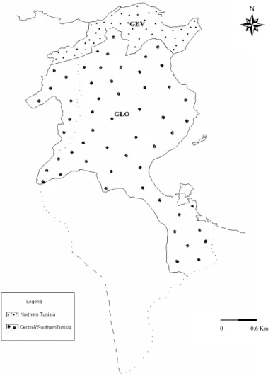
ing the boundaries of the previously delineated regions. The final delineation is pre-sented in Fig. 2 and the corresponding H values are 1.9 and 0.68 for northern and central/southern Tunisia respectively.

Figures 3 to 5 compare the observed relationships between kurtosis and L-skewness of annual maximum flood flows with the theoretical probability distributions:

5

GLO, GEV, GPA, P III, and GN. Also shown on the same figures are the locally weighted scatterplot smoothings (LOWESS) of L-skewness/L-kurtosis data, with the correspond-ing correlation coefficients. The distributions selected based on this graphical exercise, are GLO for the whole country and central part and GEV for northern Tunisia. The distribution selection from L-moment ratio diagrams was confirmed using the Z-test.

10

The distribution selection from L-moment ratio diagrams was confirmed using the Z-test. The only exception was for Central and Southern Tunisia, where L-moment ratio diagrams using LOWESS, yielded GN distribution and Z-tests resulted in recommend-ing GLO distribution. Since the distributions selected from L-moment ratio diagrams using LOWESS, as was recommended by Peel (2001), should only be used for

het-15

erogeneous zone, the Z-test selection is considered more appropriate. The average Weighted L-Skewness and L-Kurtosis for the region was also represented in the dia-gram. Therefore GLO distribution is assigned to central and southern Tunisia.

The final outcome of both L-moment diagram and Z statistical test is therefore the distribution GEV for northern Tunisia and GLO for central Tunisia. These zones are in

20

fact, characterized by relatively different physiographic and climatic conditions, which reflects the importance of these characteristics in selecting the appropriate flood fre-quency model.

8 Conclusions

Flood frequency analysis procedure was adopted to identify appropriate distributions

25

for arbitrarily delineated zones within Tunisia. Hosking and Wallis (1993) statistical measures were used to eliminate grossly discordant sites from the analysis, determine

(15)

HESSD

4, 957–981, 2007

Full Screen / Esc

EGU

the extent of heterogeneity for a given study region, and test the goodness-of-fit of a particular flood frequency distribution to observed data. Distributions were selected from L-moment diagrams, based on a comparison between the line of best fit through the data points and theoretical distribution curves.

Unlike similar previous work, such as the studies by Vogel et al. (1993b) and Vogel

5

and Wilson (1996), in which flood frequency distributions were determined for all of Australia and the United States respectively, Tunisia, in this study, was divided into two sub-regions, for which separate flood frequency analysis procedures were applied.

H-values for the study regions, describing homogeneity, generally increase from south to north. Spatial trends, with respect to best-fit flood frequency distribution, were

10

identified. Northern Tunisia was found to be represented by GEV distribution, while the GLO distribution was shown to be most suitable for the center and the south of the country.

References

Abdul Karim, M. and Chowdhury, J. U.: A comparison of four distributions used in flood

fre-15

quency analysis in Bangladesh, Hydrological Sciences, 40(1), 55–66, 1995.

Alila, Y. and Mtiraoui, A.: Implications of heterogeneous flood-frequency distributions on tra-ditional stream-discharge prediction techniques, Hydrological Processes, 16, 1065–1084, 2002.

Beard, L. R.: Flood flow frequency techniques, Center for research in water Resources, The

20

University of Texas at Austin, 1974.

Benson, M. A.: Uniform flood frequency estimation methods for federal agencies, Water Re-sources Research, 4(5), 891–908, 1968.

Bobee, B. and Rasmussen, P. F.: Reviews of Geophysics, US National Report, twent-first General assembly, International Union of Geodesy and Geophysiscs, Boulder, Colorado,

25

1111–1116, 1995.

Cathcart, J. G.: The effects of scale and storm severity on the linearity of watershed response revealed through the regional L-moment analysis of annual peak flows, Ph.D Thesis, Institute of Resources and Environment, University of British Columbia, Canada, 2001.

(16)

HESSD

4, 957–981, 2007

Full Screen / Esc

EGU

Cong, S., Li, Y., Vogel, J. L., and Schaake, J. C.: Identification of the underlying distribution form of precipitation by using regional data, Water Resources Research, 29(4), 1103–1111, 1993.

Cunnane, C.: Statistical distributions for flood frequency analysis, Operational hydro. Rep. No. 33, World Meteorological Org. (WMO), Geneva, Switzerland, 1989.

5

Farquharson, F. A. K., Green, C. S., Meigh, J. R., and Sutcliffe, J. V.: Comparison of flood fre-quency curves for many different regions in the world, in: Regional flood frefre-quency analysis, edited by: V. P. Singh, D. Reidel Publishing Co., Dordrecht, Holland, 223–256, 1987.

Finlayson, B. L. and McMahon, T. A.: Global runoff Encyclopedia of earth system science, volume 2, Academic Press Inc., San Diego, Calif., 1992.

10

Gingras, D. and Adamowski, K.: Coupling of non-parametric frequency and L-moment analysis for mixed distribution identification, Water Res. Bull., 28(2), 263–272, 1992.

Gupta, V. K., Mesa, O. J., and Dawdy, D. R.: Multiscaling theory of flood peaks: Regional quantile analysis, Water Resources Research, 30(12), 3405–3421, 1994.

Gunasekara, T. A. G. and Cunnane, C.: Split sampling technique for selecting a flood frequency

15

analysis procedure, J. Hydrol., 130, 189–200, 1992.

Hosking, J. R. M.: L-moments: analysis and estimation of distributions using linear combi-nations of order statistics, Journal of the Royal Statistical Society, Series B, 52, 105–124, 1990.

Hosking, J. R. M. and Wallis, J. R.: Regional flood-frequency analysis using L-moments,

Re-20

search Report, RC 15658, IBM Research, Yorktown Heights, New York, 1990.

Hosking, J. R. M. and Wallis, J. R.: Some statistics useful in regional frequency analysis, Water Resources Research, 29(2), 271–281, 1993.

IEA (Institution of Engineers, Australia): Australia rainfall and runoff: Flood analysis and design, IEA, Canberra, 1977.

25

Jingyi, Z. and Hall, M. J.: Regional flood frequency analysis for the Gan-Ming River basin in China, J. Hydrol., 296(1–4), 98–117, 2004.

Klemes, V.: Tall tables about tails of hydrological distributions I, J. Hydrol. Eng., 5(3), 227–231, 2000a.

Klemes, V.: Tall tables about tails of hydrological distributions II, J. Hydrol. Eng., 5(3), 232–239,

30

2000b.

Kritsky, S. N. and Menkel, F. M.: On principles of estimation methods of maximum discharge, IAHS Publ., Vol. 84, 1969.

(17)

HESSD

4, 957–981, 2007

Full Screen / Esc

EGU

McMahon, T. A. and Srikanthan, R.: Log Pearson III distribution – is it applicable to flood frequency analysis of Australian streams?, J. Hydrol., 52, 139–147, 1981.

McMahon, T. A., Finlayson, B. L., Haines, A. T., and Srikanthan, R.: Global runoff – continen-tal comparisons of annual flows and peak discharges, Catena Verlag, Cremlingen-Destedt, Germany, 1992.

5

Nathan, R. J. and Weinmann, P. E.: Application of at-site and regional flood frequency analysis, Proceeedings of the International Hydrology and Water Resources Symposium, 769–774, 1991.

NERC: Flood studies report: volume I, hydrological studies, Natural Environment Research Council, London, England, 1975.

10

Nguyen, V-T-V: On Regional Estimation of Floods for Ungaged Sites, Asia Oceania Geo-sciences Society, McGill University, Singapore, 2006.

Onoz, B. and Bayazit, M.: Best fit distributions of largest available flood samples, J. Hydro., Amsterdam, The Netherlands, Vol. 167, 195–208, 1995.

Pearson C. P.: New Zealand regional flood frequency analysis usingL-moments, J. Hydrol.,

15

30(2), 53–63, 1991.

Peel, M. C., Wang, Q. J., Vogel, R. M., and McMahon, T. A.: The utility of L-moment ratio diagrams for selecting a regional probability distribution, Hydrological Sciences, 46(1), 147– 155, 2001.

Pilon, P. J. and Adamowski, K.: The value of regional information to flood frequency analysis

20

using the method of L-moments, Canadian Journal of Civil Engineering, Ottawa, Canada, 19, 137–147, 1992.

Pilon, P. J. and Harvey, K. D.: Consolidated frequency analysis, Reference manual, Envirinment Canada, Ottawa, Canada, 1994.

Rakesh, K. and Chandranath, C.: Regional Flood Frequency Analysis Using L-Moments for

25

North Brahmaputra Region of India, J. Hydrologic Engrg., 11(4), 380–382, July/August, 2006.

Rao, A. R. and Hamed, K. H.: Regional frequency analysis of Wabash River flood data by L-moments, J. Hydrol. Eng., 2(4), 169–179, 1997.

Vogel, R. M. and Fennessey, N. M.: L-moment diagrams should replace product moment

dia-30

grams, Water Resources Research, 29(6) 1745–1752, 1993.

Vogel, R. M., Thomas Jr., W. O., and McMahon, T. A.: Flood flow frequemcy model selection in Southwestern United States, Journal of Water Resources Planning and Management,

(18)

HESSD

4, 957–981, 2007

Full Screen / Esc

EGU

ASCE, 119(3), 353–366, 1993a.

Vogel, R. M., McMahon, T. A., and Chiew, F. H. S.: Floodflow frequency model selection in Australia, J. Hydro., Amsterdam, The Netherlands, 146, 421–449, 1993b.

Vogel, R. M. and Wilson, I.: Probability distribution of annual maximum, mean, and minimum streamflows in the United States, J. Hydrol. Eng., 1(4), 69–76, 1996.

5

Wallis, J. R.: Catastrophes, computing and containment: living with our restless habitat, Spec-ulation in Science and Technology, 11(4), 295–324, 1988.

(19)

HESSD

4, 957–981, 2007

Full Screen / Esc

EGU

Table 1. Previous L-moment based flood frequency studies.

Location Number of Recommended Reference

stations distribution

Eastern United States 55 GEV Wallis (1988)

Central Victoria, Australia 53 GEV Nathan and Weinmann (1991)

South Island, New Zealand 275 EV1, EV2, and GEV. Pearson (1991)

New Brunswick, Canada 53 GEV Gingras and Adamowski (1992)

Nova Scotia, Canada 25 GEV Pilon and Adamowski (1992)

Southwestern United States 383 LN2, LN3, GEV, and LP3 Vogel et al. (1993a)

Australia 61 GEV, GAP, LP3, and LN3 Vogel et al. (1993b)

United States 1455 LN3, GEV, and LP3 Vogel and Wilson (1996)

(20)

HESSD

4, 957–981, 2007

Full Screen / Esc

EGU

Table 2. Properties of the stream flow data.

Region Number of Maximum record Number of Average record stations length (years) site years length (years)

Tunisia 31 72 799 25.8

Northern Tunisia 17 52 437 25.7 Central Tunisia 10 42 231 23.1 Southern Tunisia 4 72 131 32.8

(21)

HESSD

4, 957–981, 2007

Full Screen / Esc

EGU

Table 3. Homogeneity and goodness-of-fit tests results.

Simulation Region Average Average H-value Best-fit Z-value experiment L-skewness L-kurtosis distribution

1 Tunisia 0.391 0.261 2.02 GLO 0.35 2 Northern Tunisia 0.322 0.219 2.63 GEV −0.18 Central Tunisia 0.448 0.296 0.57 GLO −0.02 Southern Tunisia 0.521 0.340 −0.04 GLO 0.08 3 Northern Tunisia 0.333 0.217 1.90 GEV 0.09 Central/Southern 0.426 0.287 0.68 GLO −0.02 Tunisia

(22)

HESSD

4, 957–981, 2007

Full Screen / Esc

Printer-friendly Version Interactive Discussion EGU N 0 0.4 Km

Figure 1: Physiographic zones of Tunisia. Fig. 1. Physiographic zones of Tunisia.

(23)

HESSD

4, 957–981, 2007

Full Screen / Esc

Printer-friendly Version Interactive Discussion EGU N 0 0.6 Km

Figure 2: The final classification of homogeneous regions adjusted for L- Skewness and L-

Fig. 2. The final classification of homogeneous regions adjusted for Skewness and L-Kurtosis.

(24)

HESSD

4, 957–981, 2007

Full Screen / Esc

EGU

(25)

HESSD

4, 957–981, 2007

Full Screen / Esc

EGU

(26)

HESSD

4, 957–981, 2007

Full Screen / Esc

EGU