HAL Id: halshs-00564567
https://halshs.archives-ouvertes.fr/halshs-00564567
Preprint submitted on 9 Feb 2011HAL is a multi-disciplinary open access archive for the deposit and dissemination of sci-entific research documents, whether they are pub-lished or not. The documents may come from teaching and research institutions in France or abroad, or from public or private research centers.
L’archive ouverte pluridisciplinaire HAL, est destinée au dépôt et à la diffusion de documents scientifiques de niveau recherche, publiés ou non, émanant des établissements d’enseignement et de recherche français ou étrangers, des laboratoires publics ou privés.
Jean-Louis Arcand, Daniela Borodak
To cite this version:
Jean-Louis Arcand, Daniela Borodak. Explaining Productivity Differentials in Eastern European Agriculture: Efficiency or Class Structure ?. 2011. �halshs-00564567�
Document de travail de la série Etudes et Documents
E 2006.12
Explaining Productivity Differentials
in Eastern European Agriculture:
Efficiency or Class Structure ?
† Jean-Louis ARCAND and DanielaBORODAK21 p.
CERDI-CNRS, Université d’Auvergne 65, boulevard François Mitterrand 63000 Clermont Ferrand - FRANCE
Tel: (+33-4) 73431200 Fax: (+33-4) 73431228 Email(Borodak) : [email protected] Email(Arcand) : [email protected]
http://www.u-clermont1.fr/cerdi/
† The data in this study derive from a farm survey conducted by the World Bank in Moldova from February to
April 1997, and are used with their permission. The findings, interpretations, and conclusions are the authors’ own and should not be attributed to the World Bank, its Board of Directors, its management, or any member country. We thank the World Bank for making the data available, as well as participants in the CERDI development workshop for useful comments on an earlier draft. We acknowledge Zvi Lerman and Jo Swinnen for their advice and help at the very beginning of our research.
Abstract
This paper considers whether it is differences in technical efficiency or differences in factor endowments that explain productivity differentials in Moldovan agriculture. We compute non-parametric measures of technical efficiency for a sample of Moldovan small-holders using the four-step Data Envelopment Analysis (DEA) approach suggested by Fried, Schmidt and Yaisawang (1999). We also consider a model of class structure inspired by the work of Eswaran and Kotwal (1986), and estimate a bivariate probit model that explains a household's labor market participation decisions (and hence class membership) in terms of its factor endowments. These constructs are then used in an effort to understand the determinants of output per hectare in Moldovan agriculture. We find that differences in technical efficiency explain very little of the great heterogeneity in productivity observed in our sample, while class membership is slightly more successful. Our empirical model of class structure suggests that self sufficient households will disappear and be replaced by a class of small capitalist farmers as land and credit markets develop.
Key words: transaction costs, technical efficiency, household model, transitional economy, agrarian reform
1.INTRODUCTION
This paper considers the determinants of agrarian organization and productivity in transition economies, focusing on the specific case of Moldova. The debate is a particularly interesting one, first because it highlights the relative advantages of different empirical approaches and, second, because implications of the competing approaches in terms of the future evolution of agrarian structure are fundamentally different. The basic question we seek to answer is the following: what determines productivity differentials among small-scale producers in Moldova ?
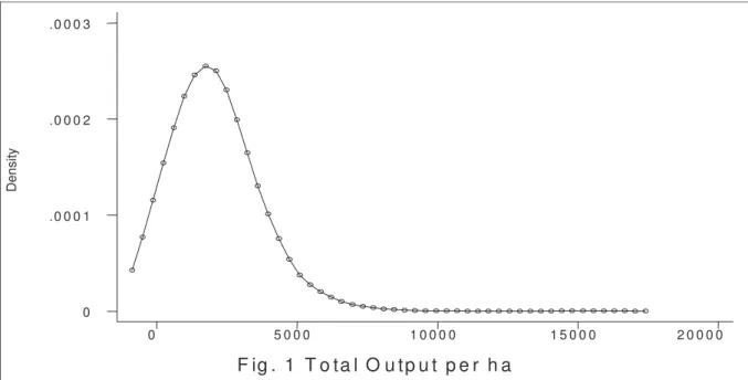
In order to provide some empirical motivation for what follows, Figure 1 displays a kernel density estimate of output per hectare for a sample of 1,019 Moldovan small-holders in 1996 and highlights the great dispersion in productivity. There are at least two ways in which these productivity differentials may be explained. First, it may be that there are important differences in the efficiency of producers. Differences in the relative deviation with respect to the efficient frontier will then explain productivity differences. This has been the explanation chosen by most authors working on the agricultural sector of transition economies. Second, it may be that there are significant differences in input choices among producers, although production decisions do lie on the relevant isoquant (frontier). These explanations are not mutually exclusive in that it may be a combination of heterogeneity in productive efficiency and in input use that explains observed productivity differentials. In this paper, one of our aims is to disentangle these two competing explanations and to assess their relative importance.
In the present paper, it will be shown, at least for the case of Moldova, that non-parametric methods (Data Envelopment Analysis) commonly used in the study of the efficiency of agricultural producers in transition economies provide only part of the explanation for observed differences in productivity among small farmers. In producer theory parlance, this means that the distance from the isoquant constitutes only a small part of what differentiates producers. Given that measures of technical efficiency for Moldovan small-holders are extremely concentrated and display relatively little heterogeneity, it is not surprizing that these measures of efficiency are not able to explain a very important portion of the observed heterogeneity in productivity.
Our complementary explanation for productivity differentials is based on a model of class structure. Differences in constraints faced by producers, particularly in terms of access to credit, lead to different degrees of participation in the labor market which in turn lead to productivity differentials. These productivity differentials are entirely consistent with productive efficiency (in the sense of being on the isoquant) and follow from differences in factor endowments.
If differences in productive efficiency do not explain an important portion of productivity differentials among producers, it follows that class membership may provide part of the answer to the productivity puzzle. Access to credit is one important factor that may determine class membership. Factors that will lead to farmers moving from one class to another will then constitute one of the channels through which the overall productivity of Moldovan agriculture will evolve.
A case in point is provided by farmers who are in a state of autarky in that they do not participate at all in the labor market: we find that the probability of a farmer belonging to this class is a decreasing function of access to credit and land ownership. This suggests, as the land sale market is liberalized (and more productive producers buy out less productive ones), that there will be a decrease in the relative importance of this class of producers, who also display the lowest productivity levels. Average productivity in the agricultural sector will then increase not because producers become more efficient, but rather because constraints that affect their participation on factor markets are loosened thereby allowing them to reduce the deviation with respect to the first-best optimum.
The relative efficiency of producers in transition economies
Most of the literature on the agricultural sector in transition economies has been concerned with measuring the relative efficiency of different types of producers. In particular, a number of studies have considered the relative efficiency of large collective farms versus that of small-scale producers, using either non-parametric methods (Data Envelopment Analysis) or parametric (stochastic frontier) approaches. Representative studies include Mathijs and Swinnen (2001), Mathijs et Vranken (1999), Piesse, Thirtle et Turk (1996), Brooks et Meurs (1994) and Brada et King (1993).
Though interesting, these results suffer from a fundamental flaw : it is inappropriate to compute measures of relative efficiency through methods such as DEA while pooling producers with intrinsically different organizational forms. In other words, while one may compute the relative efficiency of different large-scale farms with respect to each other, and do the same for small-scale producers, one may not directly compute relative efficiency measures in a dataset that includes both categories of producers. Parametric methods such as the estimation of production or cost frontiers over a heterogeneous sample of large and small producers are also inappropriate in that the underlying assumption is that they share the same production technology (the deterministic portion of the frontier): this assumption is patently untenable. It is therefore not possible to provide an empirically motivated answer to the question of whether large (ex collective) farms are more or less efficient than small-scale producers. On the other hand, it is possible to analyze the relative degree of inefficiency of small-scale producers as a group, and to analyze the determinants of any differences that may be detected.
2.NON-PARAMETRIC APPROACHES
Differences in the efficiency of farms can be attributed to two distinct sets of factors: (i) intra-farm characteristics, and (ii) inter-intra-farm differences in the environment. The ranking computed by traditional DEA methods does not allow one to distinguish between these two sources of differences in efficiency. The four-step methodology recently proposed by Fried, Schmidt and Yaisawang (1999) does.
In the first step, one computes conventional efficiency scores using the standard input-oriented DEA method. This approach would appear to be that most appropriate to agricultural producers in transition economies since their oft-stated objective is to maintain a given level of output while facing shortages of various inputs. We assume variable returns to scale (Banker, Charnes and Cooper, 1984), allowing us to compute technical efficiency scores purged of scale efficiency effects. This first stage yields conventional efficiency scores as well as a total input slack for each of the inputs under consideration.
In the second step, each total input slack is regressed on a set of variables that characterise the environment faced by the farm. Given that total input slacks are bounded from below by
zero, a tobit specification is appropriate. This second stage allows conventional statistical inference regarding the determinants of each of the total input slacks.1
Different environmental factors have been suggested in the literature. In the present context, we consider seven factors: (i) human capital (years of education of the head of the farm), (ii) age of the farm, (iii) the availability of credit (a dummy variable equal to one when the farm can obtain credit), and the quantity of credit obtained, (iv) government aid received, (v) the level of investments undertaken, (vi) non-farm income available (constituted in large part by migrant remittances), (vii) the amount of land tax paid and (viii) the availability of irrigation equipment, electricity, water and roads, as well access to common property resources.
Factors (iii) and (iv) (government aid and credit) represent a softening of the budget constraint and, according to the usual incentive arguments, should increase inefficiency. Factors (v) and (viii) (investment, irrigation, etc.), on the other hand, should be associated with a decrease in inefficiency. Factor (vii) (land tax) should increase inefficiency through the usual distortionary effects of taxation. Factor (i) (human capital) is expected to increase efficiency, but is sometimes associated with perverse effects in the context of developing country agriculture.
There remains factor (vi) (non-farm income). On the one hand, a rise in non-farm income should render the credit constraint faced by the farm less binding and should increase wastage and therefore inefficiency. On the other, non-farm income may not be treated as part of revenue in the credit constraint, especially when it stems from migrant remittances. This is because migrant remittances, in many contexts, are allocated (sometimes explicitly by the migrant) to productive investments on the farm. As such, an increase in this form of revenue may be associated with investment activity and thus with an increase of efficiency.
In the third step, one computes adjusted inputs, defined as the observed level of the input, plus the difference between the maximum fitted value of the input slack and the fitted value of the input slack for the producer in question. Since the maximum fitted value of the input slack corresponds to the worst environment faced by any farm in the sample, this step effectively
1 In addition to the references cited above, several recent papers examine the determinants of technical efficiency
in agriculture. They include, Gallagher, Goetz and Debertin, 1997, Ngwenya, Battese and Fleming, 1997, and Jones, Klinedinst and Rock, 1998.
places all producers in the same conditions. Finally, in the fourth step, conventional DEA estimation is used to recomputed efficiency scores, where one uses the adjusted inputs in place of the actual inputs.
3.THE RELATIVE EFFICIENCY OF SMALL-SCALE PRODUCERS:
EMPIRICAL RESULTS FOR MOLDOVA
The data used in this paper stem from a survey undertaken by the World Bank and the Agency for Agricultural Restructuring between February and April 1997, at which point the reform process in Moldova was well underway. The survey covers 28 out of 36 districts over the three agro-climatic zones (North, Center, South) of the country. Small farms included in the survey were randomly drawn at the village level.
As of mid-1996, 91.4% of agricultural land was deemed to have been "privatized" and 983,000 households had rights to a land share. These ownership certificates represented a total of 2.2 million plots of land with the average plot size being 1.5 hectares. These figures are somewhat misleading since, as of April 1998, only 21% of land was being cultivated as household plots or as independent family farms. Many kolkhozes had already been technically dismantled but continued apparently to appropriate a large share of arable land. Most (95%) of the small-holders included in our sample engage in agricultural production and animal husbandry. Most (94%) of these producers operate on the plots that were redistributed to peasants during the privatization process, with an average farm size of 2.4 hectares. For the remainder, who rent in land, average farm size was of 7.5 hectares (the average amount of land rented in was equal to 4.2 hectares).
Agricultural technology used by Moldovan small-holders follows traditional patterns although some producers do use chemical fertilisers and new seed varieties. Individuals who are members of large (former collective) farms enjoy preferential access to subsidized inputs to be used on their own household plots which explains their continued membership in these organizations. Agricultural machinery was largely distributed to the former collective farms: among small-holders, only 10% possess a tractor.
presented in Table 1. The mean initial and adjusted efficiency score for small farms are 52% and 91%, respectively. As is obvious from the kernel estimates presented in Figure 2, adjusting our estimates of technical efficiency so that all small-holders are placed within the same environment leads to a highly concentrated distribution: the standard deviation of adjusted technical efficiency is equal to 0.06. Moreover, the minimum level of adjusted technical efficiency is equal to 67%. There is thus relatively little scope for increasing the productivity of Moldovan small-holders by increasing their technical efficiency, at least as far as the full sample results are concerned.
Determinants of total input slacks
Though increasing technical efficiency may not offer the most promising manner of improving the overall productivity of Moldovan small-holders it is nevertheless interesting to understand what lies behind these adjusted measures, as those variables that are significant determinants of raw technical efficiency may be amenable to policy interventions. Table 2 reports results corresponding to the second stage of the procedure, whereas Table 3 presents the corresponding marginal impacts of the explanatory variables. A positive coefficient means that an increase in the variable in question leads to an increase in the total slack and thus to a fall in efficiency.
Surprisingly, human capital, represented by the number of years of education of the farm head, has no statistically significant impact on the total input slacks.2 The use of irrigation, on the other hand, reduces inefficiency associated with the use of the land input (as well as other, non-labor, inputs). Unsurprisingly, the distortionary effect of taxation, and its impact on efficiency is apparent: the amount paid in land taxes increases the total slack associated with all three factor inputs.
Credit availability, as well as the amount of credit received, in conformity with the soft budget constraint view that is often alluded to in order to explain inefficiency, increases the total slack associated with the land input and with other inputs. The same is true for the amount of government aid received by the farm (all three total slacks are increased). On the other hand, revenue stemming from non-agricultural activities (including transfers from migrants)
2 Mathijs and Vranken (1999) found a statistically significant effect of education on total technical efficiency for
improves the efficiency with which land and labor are utilized (while its impact on other inputs is the opposite). Similarly, an increase in farm investments increases the efficiency with which all three inputs are utilized.
These results suggest an important distinction. While it is true that an increase in credit availability can, potentially, lead to an increase in productive efficiency through a relaxation of the farm’s resource constraint, the fact that credit increases inefficiency when one controls for investment indicates that it is the disincentive effect of the soft budget constraint that dominates, by reducing competitive pressures on the farm. The same argument holds for government aid. On the other hand, it may at first seem surprising that non-agricultural income decreases inefficiency, especially in light of the negative impact of government aid and credit. This result becomes less surprising when one keeps in mind that diversification of activities may reflect a high degree of managerial initiative, as well as the fact that a major component of non-agricultural income —migrant remittances— are often specifically earmarked for productive investment uses. The upshot is that resources, at least in the case of Moldovan agriculture, are manifestly not fungible.
Can differences in efficiency explain differences in productivity ?
In order to assess whether differences in efficiency can provide one with a coherent explanation for the observed heterogeneity in the productivity of Moldovan small-holders, we regress output per hectare on our adjusted measure of efficiency. If differences in efficiency constitute an important piece of the productivity puzzle, one would expect that they would be able to explain an important portion of differences in productivity. As should be obvious from the results presented in the first column of Table 5, this is not the case. Although adjusted technical efficiency does constitute a statistically significant determinant of agricultural productivity (output per hectare), it is able to account for only an infinitesimal share of that variable's variance (as evidenced by the extremely low R-squared). Other factors, outside of differences in technical efficiency per se, must therefore lie behind the great heterogeneity in the productivity of Moldovan small-holders.
4.HOUSEHOLD MODELS AND CLASS STRUCTURE
One of the most useful corollaries of the unitary household model of agricultural production that is extensively used in development microeconomics is constituted by models of class structure. Building on the seminal contributions of Roemer (1982) and Bardhan (1982), Eswaran and Kotwal (1986) develop a household model in which credit constraints, coupled with supervision costs on hired labor, generate a taxonomy of peasant classes that are differentiated according to their participation on either side of the labor market. Other models of class structure permit one to investigate the determinants of participation on other factor markets, such as the land rental market, or of the ability of farmers to commercially market their output. The Eswaran-Kotwal (1986) model, in particular, predicts productivity differentials generated by class membership which in turn is determined by factor endowments. Carter and Wiebe (1990) and Wydick (1999) focus on the impact of the access to credit on the productivity of farmers, as well as on class membership.
One commonly-noted feature of the organizational structure of the agricultural sector in transition economies following decollectivization is the emergence of different classes of farmers characterized by differing degrees of participation on various markets. While the process of decollectivization and the distribution of land titles was often driven by egalitarian goals, a good deal of heterogeneity has already emerged, leading rapidly to polarization into easily recognizable classes of producers. In the case of Moldova, a number of class taxonomies are possible. In what follows, we focus, in the tradition of Eswaran and Kotwal, on a model with four classes defined by the hiring in and hiring out of labor.
Class structure: a model for Moldova
Consider a simple unitary household model where a household's inelastically supplied endowment of labor will be denoted by L and its endowment of land by T . The production technology will be represented by a Cobb-Douglas specification in which family labor and land are essential inputs, whereas hired labor may be dispensed with if it is so desired. We express this by writing the production technology as q
(
1 Lin)
L Tα β γ
= + , where L is hired in
labor, L is family labor used on the farm, and T is the size (in hectares) of the farm. The rental prices of labor will be assumed to differ depending upon whether one is hiring in (w1)
or hiring out (w2), where we assume that w2 < . The rental price of land will be denoted by w1
r and we choose agricultural output as the numeraire. Apart from the technology of production, the household is potentially constrained by the availability of working capital or, in other words, credit. We express this writing
1 in 2( ) ( )
w L −w L L− +r T T− ≤B,
the usual assumption being that factor inputs must be paid for at the beginning of the season, while output, and hence liquidity, obtains only at the end. In the preceding inequality, B
denotes available liquidity. Note that this credit constraint can be re-expressed as
1 in 2 2
w L +w L rT+ ≤ +B w L rT+ .
That is, production costs (on the left-hand-side) must be less than or equal to total available liquidity, given by the rental value of the household's endowment of labor and land plus available short-term credit (which may be constituted by a roll of bills under the bed). The household's optimization problem is then posed as follows:
{ , , }
(
)
1 2 1 2 max 1 ( ) ( ) ( ) ( ) ; . . 0; . in in in L L T in in L L T w L w L L r T T w L w L L r T T B s t L L L α β γ + − + − − − − − + − ≤ ≥ ≥There are potentially eight classes in this model since there are 3 constraints (8 2= 3). We will abstract from these concerns and consider the cases which correspond to a binding credit constraint.3 When this is case, we can solve out for the amount of land being farmed, and transform our initial problem into the following maximization program:
{ }
(
)
1 2 , max 1 ( ) in in in L L w w B L L L L L T r r r γ α β + − + − + .If we allow the two remaining constraints to hold with strict inequalities, the corresponding first-order conditions (FOCs) allow one to write:
(
)
(
1 2)
2 B w w L rT L wβ
α β γ
+ + + = + + , 1 1 1 2 1 in w B w w L rT Lα
α β γ
− + + + = − + + , and 1 1 2 B rT w w L r Tγ
α β γ
− + + + = + + .The household will "import" labor whenLin > , which corresponds to the condition that 0 1 1 1 2 1 0 w B w w L rT
α
α β γ
− + + + − > + + .Rearranging this expression yields (1) B rT+ >
β γ
α
+ w w L1− 2 .Conversely, the household will "export" labor when its endowment of labor is greater than the amount of labor it desires to use on its own farm: L L− >0. This can be written as
(
)
(
1 2)
2 0 B w w L rT L wβ
α β γ
+ + + − > + + , which simplifies to (2) B rTα γ
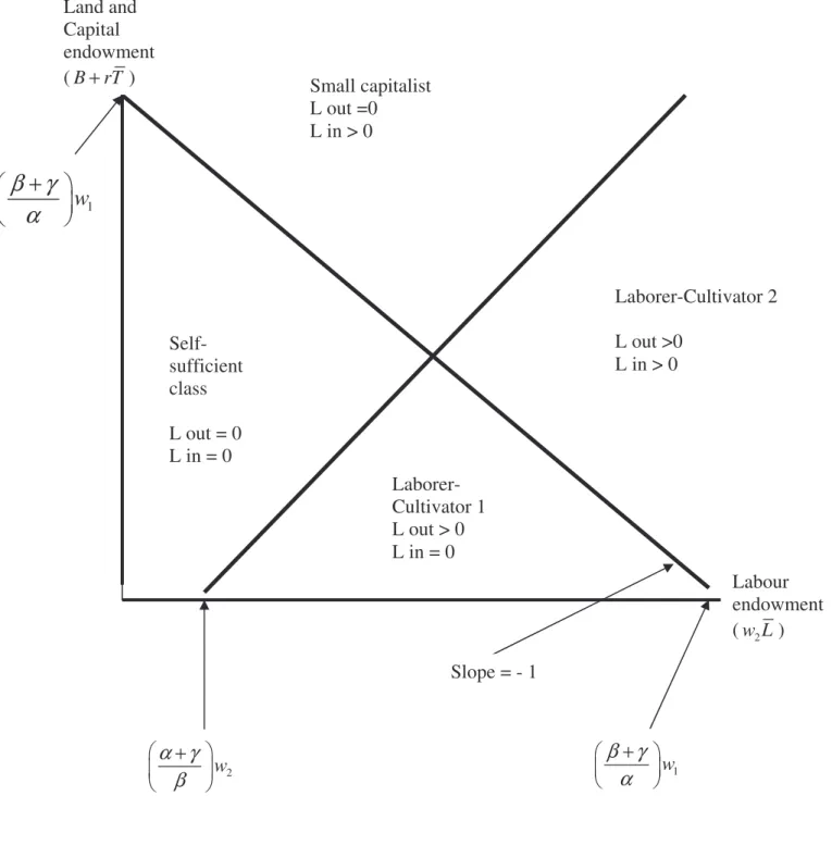
w L w2 1β
+ + < − .These two conditions are represented graphically in (w L B rT2 ; + ) space in Figure 3, with four classes emerging, corresponding to (i) autarky (Lin =0,Lout = ), (ii) type 1 labourer 0 cultivators (Lin =0,Lout > ), (iii) type 2 labourer cultivators (0 Lin >0,Lout > ), and (iv) small 0
capitalists (Lin >0,Lout = ).0 4
5.CLASS STRUCTURE:EMPIRICAL RESULTS FOR MOLDOVA
Table 4 provides empirical results from a bivariate probit model that represents the conditions given by equations (1) and (2). Ceteris paribus, our theoretical model leads us to expect that the probability of labor being hired in is a decreasing function of the labor endowment of the household and an increasing function of its endowment of land and its access to working capital. Conversely, the probability of hiring out family labor should be increasing in the household's endowment of labor, and decreasing in its land ownership and access to working capital. A number of additional explanatory variables, particularly those linked to the human capital and previous experience of the household head, are included as controls.
As should be clear from the empirical results, the predictions of the theoretical model are confirmed by our estimates. The probability of hiring in is a decreasing function of family
size (measured by the number of economically active family members) and an increasing function both of land ownership (in hectares) and exogenous (i.e., non-agricultural) income.5
All of these effects are statistically significant at the usual levels of confidence. The converse is true of the probability of hiring out and, once again, all of the relevant effects are statistically significant at the usual levels of confidence.
In order to address our initial question of what lies behind the great heterogeneity in the output per hectare of Moldovan small-holders, Table 5 presents results where the dependant variable is output per hectare and explanatory variables include the household's factor endowments and available credit, as well as its adjusted technical efficiency score. Note that we carry out four regressions, corresponding to each of the four classes suggested by our theoretical model of class structure. In order to control for potential sample selection bias, we include the predicted probability of a given household belonging to the class in question computed from the bivariate probit results presented in Table 4.6
The first important result to retain from Table 5 is that, once one controls for class structure and household endowments, technical efficiency is no longer a statistically significant determinant of output per hectare (the lowest p-value associated with this variable obtains in the type 2 laborer-cultivator class and is equal to 0.261). In contrast, membership in a class per se (the coefficient associated with the predicted probability) is statistically significant in all but the small capitalist equation. This is particularly true of the self sufficient class (households who choose to remain autarkic). Second, the relaxation of a household's credit constraint increases output per hectare for type 1 laborer-cultivators, whereas it reduces output per hectare for small capitalists. Third, an increase in the endowment of land decreases output per hectare for type 1 laborer-cultivators. Fourth, the output per hectare of small capitalists is an increasing function of the household's labor endowment. It is worth noting that a disappointing aspect of these estimation results is that the explanatory power of the specification is extremely low, with the adjusted R-squared never exceeding 0.05.
In terms of the future evolution of the aggregate productivity of Moldovan agriculture, one must take care to interpret the bivariate probit results before turning to the productivity equations. For example, consider the impact of an increase in the availability of credit to self
5 We cannot consider agricultural or wage income as they are endogenous variables in the model. 6 As such, these estimation results resemble those carried out in tests of "selective separability".
sufficient producers. While credit does not have a statistically significant impact on the output per hectare of self sufficient producers, an increase in credit availability will tend to move members of this class toward the small capitalist class (a vertical shift in Figure 3). If there is an "insufficient" number of household's in the small capitalist class with respect to the self sufficient class in that the marginal productivity of land is higher for the former than for the latter, then this shift in class structure should move one towards the equalization of the marginal productivity of land (and hence increase the aggregate output stemming from these two classes recall that the optimal allocation of land is obtained when its marginal productivity is equated across classes).
6.CONCLUDING REMARKS
The purpose of this paper was to understand why there is a great dispersion in the productivity of small-holders in Moldova. Two competing explanations were considered. First, that productivity differences are driven by differences in technical efficiency, which has been the focus of much of the empirical literature on the agricultural sector of transition countries in Eastern Europe and the FSU. Second, that productivity differences can be explained in terms of class structure, where class structure emerges as a result of market imperfections (particularly in terms of access to credit) and differences in the relative factor endowments of different producers. Our empirical results highlight that differences in technical efficiency do not furnish one with a sound explanation for productivity differentials and that, while class structure does contribute something, it does not represent as yet a satisfactory answer.
Though the productivity puzzle remains just that —a puzzle— this paper does provide answers to two important questions concerning the transition process in Eastern Europe and the FSU, at least as far as the example of Moldova can be generalized. To the question : "Can small producers escape the fetters of autarky and improve their productivity ?" our answer is yes, as long as the land market is liberalized and access to credit is improved, since this will tend to transform self sufficient producers into what Eswaran and Kotwal (1986) refer to as "small capitalists". To the question: "Will the private agricultural sector become rapidly polarized into different agrarian classes ?" our answer is that it already is. Moreover, certain classes of producers, such as those in autarky, are destined to disappear as the reform process moves forward and the market mechanism becomes more solidly entrenched.
REFERENCES
AGENCY FOR RESTRUCTURING AGRICULTURE & WORLD BANK (1998), Moldova: Agricultural Policy Update 1997-1998, Chisinau.
BRADA, J. and A. KING (1993), “Is Private Farming More Efficient than Socialized Agriculture?” Economica, vol. 60, n 1, pp. 41-56.
BROOKS, K. and M. MEURS (1994), “Romanian Land Reform: 1991-1993,” Comparative Economic Studies, vol. 36, n 2, pp. 17-32.
ESWARAN, M. and A. KOTWAL (1986), “Access to capital and agrarian production organization,” Economic Journal 96:482-498.
FRIED, H. O., S. S. SCHMIDT and S. YAISAWARNG (1999), “Incorporating the Operating Environment into a Nonparametric Measure of Technical Efficiency,” Journal of Productivity Analysis, vol. 12, n 3, pp. 249-267.
GALLAGHER, M., S. J. GOETZ and D. L. DEBERTIN (1997), “Efficiency Effects of Institutional Factors: Limited-Resource Farms in Northeast Argentina,” in Rose, R., C. Tanner and M. A. Ballamy IAAE Occasional Paper N° 7 "Issues in Agricultural Competitiveness: Markets and Policies", The International Association of Agricultural Economists, pp. 68-76.
JONES, D., M. KLINEDINST and C. ROCK (1998), Productive Efficiency during Transition: Evidence from Bulgarian Panel Data, Journal of Comparative Economics, vol. 26, n 4, pp. 446-464.
MATHIJS, E. and J. F. M. SWINNEN (1999), “Efficiency Effects of Land Reforms in East Central Europe and the Former Soviet Union” Paper presented at the IAMO-FAO/REU seminar on “Land Ownership, Land Markets and their Influence on the Efficiency of Agricultural Production in Central and Eastern Europe”, 9-11 May, Halle/Saale, Germany.
MATHIJS, E. and J.F.M. SWINNEN (2001), “Production and Efficiency During Transition: An Empirical Analysis of East German Agriculture”, The Review of Economics and Statistics, 1(2): 100-108.
MATHIJS, E. and L. VRANKEN (1999), “Determinants of Technical Efficiency in Transition Agriculture: Evidence from Bulgaria and Hungary,” EU Phare ACE and The World Bank/ECSSD/DECRG Working Paper N° 1.
NGWENYA, S. A., G. E. BATTESE, and E. M. FLEMING (1997), “The Relationship Between Farm Size and the Technical Inefficiency of Production of Wheat Farmers in the Eastern Free State, Province of South Africa,” Agrekon, vol. 36, n 3, pp. 283-301.
PIESSE, J., C. THIRTLE and J. TURK (1996), “Efficiency and Ownership in Slovene Dairying: A Comparison of Econometric and Programming Techniques,” Journal of Comparative Economics, vol. 22, n 1, pp. 1-22.
Figure 2. Kernel Density Estimates
Distribution of Initial and Final Performance Rankings (technical efficiency, variable returns to scale)
D en si ty F ig . 1 T o ta l O u tp u t p e r h a 0 5 0 0 0 1 0 0 0 0 1 5 0 0 0 2 0 0 0 0 0 .0 0 0 1 .0 0 0 2 Table 1.
Initial and Final Results of Four-Step DEA Estimation (1019 observations)
Average Standard
Deviation Minimum
Initial
Results ResultsFinal ResultsInitial ResultsFinal ResultsInitial ResultsFinal
Total Efficiency 0.1966 0.1146 0.1342 0.0977 0.0110 0.0040
Technical Efficiency 0.5179 0.9015 0.1848 0.0647 0.1250 0.6710
Scale Efficiency 0.3868 0.1293 0.2082 0.1098 0.0340 0.0040
Technical efficiency, variable returns to scale
initial efficiency scores adjusted efficiency scores
.1 .2 .3 .4 .5 .6 .7 .8 .9
.016372 3.07314
Table 2.
Determinants of total input slacks Method of estimation: Tobit
(1019 observations, p-values next to estimated coefficients)
Dependents Variables
Total Slack
(Total Land Surface) (Permanent Workers) Total Slack (Other Inputs) Total Slack
Coefficient p-value Coefficient p-value Coefficient p-value
Constant 0.4085 0.2371 1.1550 0.0000 -1419.6 0.0003
Education of Head 0.0228 0.3753 0.0196 0.1677 116.9 0.0001 Age of the farm 0.0834 0.1115 0.0190 0.5123 11.4 0.8482 Credit (lei) 0.0000 0.8208 0.0000 0.2147 0.1 0.0297 Credit Availability(dummy) 0.5481 0.0050 0.2873 0.0073 491.5 0.0259 Government Grants (lei) -0.0010 0.4224 -0.0002 0.7478 1.4 0.1836 Investments (lei) 0.0000 0.1735 0.0000 0.7444 -0.1 0.5376 Other Revenues (lei) 0.0001 0.0339 0.0001 0.0023 0.2 0.6710 Land Tax (lei) 0.0046 0.0000 0.0007 0.0000 3.6 0.0000 Irrigation (dummy) 0.3827 0.1919 0.4627 0.0045 419.2 0.2107 Infrastructure (dummy) -0.2405 0.1970 -0.2435 0.0174 -186.5 0.3759 Equipment (dummy) -0.0115 0.9594 -0.1225 0.3272 271.5 0.2909 Region Center (dummy) -1.1302 0.0000 -0.2037 0.0316 541.2 0.0055 Region North (dummy) -0.7814 0.0001 -0.1774 0.1111 48.3 0.8327
Sigma 2.1383 0.0000 1.1870 0.0000 2441.5 0.0000
Log-likelihood -2149 -1607 -9219
Note: 1 lei = 0.22 US$, "infrastructure" corresponds to a dummy variable indicating whether electricity, water and roads are available; equipment is constructed in the same manner.
Table 3.
Determinants of total input slacks
Method of estimation: Tobit, Marginal Effects
(1019 observations, p-values next to estimated coefficients)
Dependents Variables
Total Slack
(Total Land Surface) (Permanent Workers) Total Slack (Other Inputs) Total Slack
Marginal effect p-value Marginal effect p-value Marginal effect p-value
Constant 0.3374 0.2382 1.0713 0.0000 -1070.0 0.0003
Education of Head 0.0188 0.3753 0.0182 0.1678 88.1 0.0001
Age of the farm 0.0689 0.1116 0.0176 0.5123 8.6 0.8482
Credit (lei) 0.0000 0.8208 0.0000 0.2147 0.1 0.0298
Credit Availability(dummy) 0.4528 0.0050 0.2665 0.0073 370.4 0.0260 Government Grants (lei) -0.0008 0.4223 -0.0002 0.7478 1.0 0.1837
Investments (lei) 0.0000 0.1735 0.0000 0.7444 -0.01 0.5376
Other Revenues (lei) 0.0001 0.0339 0.0001 0.0023 0.02 0.6710
Land Tax (lei) 0.0038 0.0000 0.0006 0.0000 2.73 0.0000
Irrigation (dummy) 0.3161 0.1920 0.4292 0.0045 316.0 0.2108
Infrastructure (dummy) -0.1987 0.1970 -0.2259 0.0174 -140.5 0.3760
Equipment (dummy) -0.0095 0.9594 -0.1137 0.3273 204.6 0.2909
Region Center (dummy) -0.9335 0.0000 -0.1889 0.0316 407.9 0.0055
Figure 3 : Partition of factor endowment space implied by the model of class structure
Labour endowment (w L ) 2 Land and Capital endowment ( B rT+ ) 2 w
α γ
β
+ 1 wβ γ
α
+ 1w
β γ
α
+
Slope = - 1 Small capitalist L out =0 L in > 0 Self-sufficient class L out = 0 L in = 0 Laborer-Cultivator 1 L out > 0 L in = 0 Laborer-Cultivator 2 L out >0 L in > 0Table 4.
Determinants of Class Structure: Bivariate Probit Estimation (1019 observations, p-values next to coefficients)
Dependent Variable 1 0 0 in if L y otherwise > = 1 0 0 out if L y otherwise > =
Coefficient p-value Coefficient p-value
Labor endowment -0.1074 0.0010 0.3578 0.0000
Land endowment 0.1809 0.0000 -0.0846 0.0020
Exogenous revenues (lei) 0.0000 0.1750 -0.0001 0.0590
Proportion of qualified hh. members 0.1403 0.4970 0.3285 0.1490
Education of Head -0.0153 0.4710 0.0441 0.0560
Previous employment of Head :
farm enterprise -0.2401 0.1960 -0.8266 0.0000
industrial or construction enterprise 0.0547 0.8260 -0.7914 0.0010
social services -0.1821 0.4570 -0.4028 0.1030
local administration 0.2389 0.4980 -0.5913 0.1140
Age of the farm (years) 0.0481 0.1450 0.0551 0.0790
Access to CPRs (dummy) 0.1486 0.1100 -0.0007 0.9940
Infrastructure (dummy) 0.1724 0.1140 0.0549 0.6220
Availability of technical and transport equipment (dummy) 0.2582 0.0870 -0.0373 0.7980
Constant -0.6921 0.0190 -0.5501 0.0640
Rho [p-value] -.106 [.002]
Table 5.
Determinants of Productivity: Technicial Efficiency versus Class Structure (OLS estimation with correction for sample-selection bias)
Full sample Self-sufficient Laborer-cultivator1 Small Capitalist Laborer-cultivator 2
0, 0
in out
L = L = Lin =0, Lout > 0 Lin >0, Lout = 0 Lin >0, Lout > 0
Coefficient p-value Coefficient p-value Coefficient p-value Coefficient p-value Coefficient p-value
Constant -389.3668 0.566 -17.6591 0.6510 -22.4582 0.5750 -17.6649 0.7680 6.8964 0.9220
Land endowment 11.2953 0.8650 -176.6703 0.0120 -65.5558 0.3840 -139.7731 0.3650
Labor endowment -0.0209 0.3560 -0.0266 0.6490 0.0513 0.0130 -0.0490 0.4200
Credit (lei) -547.8578 0.4380 1223.4810 0.0750 -1554.6040 0.0090 -281.3031 0.7580
Predicted probability of
belonging to the class 2918.5050 0.0090 2590.4180 0.0420 389.0946 0.8660 5529.5410 0.0280
Adjusted efficiency score
from 4-stage DEA 2743.181 0.000 -368.8586 0.7120 -71.7577 0.9520 2182.0660 0.2780 -2300.5710 0.2610
Adjusted R-Squared 0.0152 0.0248 0.0388 0.0220 0.0551