HAL Id: hal-01022470
https://hal-enac.archives-ouvertes.fr/hal-01022470
Submitted on 22 Jul 2014
HAL is a multi-disciplinary open access
archive for the deposit and dissemination of
sci-entific research documents, whether they are
pub-lished or not. The documents may come from
teaching and research institutions in France or
abroad, or from public or private research centers.
L’archive ouverte pluridisciplinaire HAL, est
destinée au dépôt et à la diffusion de documents
scientifiques de niveau recherche, publiés ou non,
émanant des établissements d’enseignement et de
recherche français ou étrangers, des laboratoires
publics ou privés.
From movement tracks through events to places :
extracting and characterizing significant places from
mobility data
Gennady Andrienko, Natalia Andrienko, Christophe Hurter, Salvatore
Rinzivillo, Stefan Wrobel
To cite this version:
Gennady Andrienko, Natalia Andrienko, Christophe Hurter, Salvatore Rinzivillo, Stefan Wrobel. From
movement tracks through events to places : extracting and characterizing significant places from
mo-bility data. VAST 2011, IEEE Conference on Visual Analytics Science and Technology, Oct 2011,
Providence, United States. pp 161-170, �10.1109/VAST.2011.6102454�. �hal-01022470�
From Movement Tracks through Events to Places: Extracting and
Characterizing Significant Places from Mobility Data
Gennady Andrienko1, Natalia Andrienko1, Christophe Hurter2, Salvatore Rinzivillo3, Stefan Wrobel1
1
Fraunhofer Institute IAIS (Intelligent Analysis and Information Systems) and University of Bonn, Germany
2
DGAC/DTI R&D, ENAC and the University of Toulouse, France
3
KDDLab, ISTI – CNR, Pisa, Italy
ABSTRACT
We propose a visual analytics procedure for analyzing movement data, i.e., recorded tracks of moving objects. It is oriented to a class of problems where it is required to determine significant places on the basis of certain types of events occurring repeatedly in movement data. The procedure consists of four major steps: (1) event extraction from trajectories; (2) event clustering and extraction of relevant places; (3) spatio-temporal aggregation of events or trajectories; (4) analysis of the aggregated data. All steps are scalable with respect to the amount of the data under analysis. We demonstrate the use of the procedure by example of two real-world problems requiring analysis at different spatial scales.
KEYWORDS: movement, trajectories, spatio-temporal data, spatial
events, spatial clustering, spatio-temporal clustering
1 INTRODUCTION
Movement data (also called mobility data) describing changes of
spatial positions of discrete mobile objects are nowadays collected in growing amounts by means of current tracking technologies, such as GPS, RFID, radars, and others. Automatically collected movement data are semantically poor as they basically consist of object identifiers, coordinates in space, and time stamps. Despite that, valuable information about the objects and their movement behavior as well as about the space and time in which they move can be gained from movement data by means of analysis [2].
Movement can be viewed as consisting of continuous paths in space and time [18], also called trajectories, or as a composition of various spatial events [3]. As noted in [6] and [30], there are many definitions of the term event. We adhere to Kim’s definition of events as exemplifications of properties or relationships at some times [22]. Spatial events are events localized in space [6].
The event-based view of movement is particularly suitable for applications and tasks where analysts are interested in occurrences of certain movement characteristics such as very high or very low speeds. Each occurrence is a spatial event. Events that are relevant to the goals of analysis need to be extracted from movement data. Such events will be further called movement events, or m-events.
There is a class of problems where analysts need to determine
places in which m-events of a certain type occur repeatedly and
then use these places in the further analysis. For example, having tracks of multiple cars in a city, a traffic analyst may first need to find places where traffic jams occur and then investigate in which times of the day they happen and how long they last. From trails of migratory birds, an ornithologist may wish to extract places
where the birds stop for resting and feeding and then analyze the temporal patterns of visiting these places and travelling between the places. We point out that relevant places can only be delineated by processing movement data, that is, there is no predefined set of places (e.g., compartments of a territory division) from which the analyst can select places of interest. The relevant places may have arbitrary shapes and sizes and irregular spatial distribution. They may even overlap in space; hence, approaches based on dividing the territory into non-overlapping areas (as in [4]) are not appropriate.
We propose a visual analytics procedure for place-centered analysis of mobility data that includes (1) visually-supported extraction of relevant m-events, (2) finding and delineating significant places on the basis of interactive clustering of the m-events according to different attributes, (3) spatio-temporal aggregation of the m-events and movement data by the defined places or pairs of places and time intervals; (4) analysis of the aggregated data for studying the spatio-temporal patterns of event occurrences and/or connections between the places. We demonstrate the use of the procedure by applying it to two real-world problems differing in the spatial scale and character of the movement that is analyzed.
The main contributions of this paper are following:
• We suggest a generic visual analytics procedure for a certain class of problems, which is explicitly specified. The existing literature describes particular techniques that can be used in different steps of the procedure. We put the techniques in a workflow, in which outputs of one technique are used as an input for another technique.
• The procedure can be scaled to large amounts of data. We explicitly describe the use of the procedure in a case when the data do not fit in the RAM (section 4.5).
• We suggest an original approach to clustering of events, which uses a special distance function capable to account for distances between events in geographic space, in time, and with regard to values of thematic attributes. The function properly deals with cyclic attributes such as movement direction or time of a day. The remainder of the paper is structured as follows. After introducing the main concepts in section 2, we discuss the related research (section 3) and describe the suggested procedure (section 4). Sections 5 and 6 present two examples of the use of the procedure; a supplement with larger figures and more details is given at http://geoanalytics.net/and/papers/vast11att.pdf. Section 7 concludes the paper.
2 MOVEMENT DATA AND POSSIBLE DERIVATIVES
Movement data consist of position records <object identifier, time,
spatial coordinates>. Temporally ordered position records of one object represent the trajectory of this object. The real trajectory is continuous (i.e., the object has some position at any time moment) while the data representing it are discrete (i.e., positions are specified for a sample of time moments). When the time intervals between the known positions are sufficiently short, the http://geoanalytics.net/and; andrienko@geoanalytics.net
IEEE Symposium on Visual Analytics Science and Technology October 23 - 28, Providence, RI, USA
intermediate positions can be estimated by means of linear or non-linear interpolation [26][2].
From reconstructed trajectories, one can compute a number of
instant, interval, and cumulative characteristics of the movement.
Instant movement characteristics include instant speed, direction, acceleration (change of speed), and turn (change of direction) [17]. Interval characteristics are computed for time intervals of a chosen constant length before, after, or around a given time moment. They include traveled distance, displacement, average speed, sinuosity, tortuousity, as well as statistics of the instant characteristics. Cumulative characteristics are computed for the interval from the start of the trajectory to a given time moment or for the remaining interval to the end of the trajectory. Cumulative measures include all interval measures and the temporal distances to the starts and ends of the trajectories.
Movement takes place in spatio-temporal context [3], which includes spatial locations and time moments or intervals with their specific properties, as well as various spatial, temporal, and spatio-temporal entities existing in the space and/or time. For each particular point or segment of a moving object’s trajectory, all previous and following movements of this object also belong to the spatio-temporal context.
As an object moves, various spatial, temporal, and spatio-temporal relations occur between this object and elements of the context. Some types of relations, such as topological relations ‘in’, ‘cross’, ‘touch’, are called qualitative [13] and are represented by predicates. Other types of relations, such as spatial and temporal distance and spatial direction, are called metric [25] and are represented by numeric-valued functions. For a selected element or set of elements of the context and a selected relation type, it is possible to compute the value of the respective predicate or function in each time moment of a moving object’s trajectory. This requires availability of data about the spatial and temporal positions of the selected context elements. For some context elements, such as other moving objects or previous movements of an object, the positions can be extracted from the set of trajectories. For other context elements, additional data (called
context data) need to be provided, for example, coordinates of
places of interest or times and locations of events of interest. Movement characteristics and relations to the context can be represented by dynamic (i.e., time-varying) attributes. Besides the attributes that can be computed from reconstructed trajectories and context data, some dynamic attributes may be originally available in the movement data. By means of queries, one can find points and segments of trajectories having particular values of one or more dynamic attributes. According to the event-based view [3], these are movement events (m-events), which can be extracted from the trajectories and analyzed independently of the set of trajectories or in combination with it.
3 RELATED WORK
There is abundant literature concerning analysis of movement, which is currently a hot research topic. Paper [2] gives a summary of major approaches and classes of techniques. Here we consider only the works strongly related to the steps of our procedure. The works are grouped according to these steps.
Extraction of events from movement data. The possibility of
extracting spatial events from different types of spatio-temporal data is discussed in [6] but concrete methods are not presented. Moving object databases [17] compute various dynamic attributes (numeric functions and predicates) and provide a powerful query language for extracting parts of trajectories based on these attributes. However, there is no convenient user interface for query specification and for viewing the results. Paper [3] describes a visual query tool that computes and visualizes some of the movement characteristics and distances to selected context
elements and filters trajectory segments according to values of one or more of the dynamic attributes. In [11], a graphical user interface is used for specifying queries in terms of instant and interval characteristics, particularly, fractal characteristics (e.g., tortuousity) expressing the geometrical complexity of trajectory segments. The tool provides an immediate visual feedback on a map display. In [16], multiple coordinated views and interactive visual queries are used for detecting microscopic traffic patterns and abnormal behaviors on a road crossing; however, filtering is applied to whole trajectories rather than segments.
In [8], relations to the spatio-temporal context are used for computational extraction of m-events from trajectories of mobile phone users. The authors extract sufficiently long stops occurring in spatial and temporal proximity to known public events. They also extract stop events occurring in the night hours in order to determine the home locations of the people. In [31], stop events are extracted from car trajectories based on the speed values; then, additional context information (e.g., points of interest) is used to separate meaningful stops from non-meaningful.
In [24] and [10], instant and interval movement characteristics are used to decompose trajectories into episodes of homogeneous movement, which are then used for detecting particular movement patterns [24] or classification of movement modes [10].
Spatial clustering of events and definition of relevant places.
Paper [15] applies density-based spatial clustering to points of multiple trajectories to delineate areas of intense traffic. Then frequent sequences of visited areas with typical transition times (T-patterns) are extracted by means of data mining methods. In [28], a specific kernel density estimation method is applied to trajectories. It allows detecting particular places, e.g., anchoring areas of ships. In [4], a special algorithm for spatially constrained clustering is applied to points extracted from trajectories. It makes clusters of desired spatial extents, which are then used for territory tessellation. Density-based clustering of trajectory points over successive time slices is used in [21] for finding moving clusters of objects rather than places of interest.
Aggregation of event and movement data. In [14], spatial,
temporal, and categorical (attribute-based) aggregation of traffic events is done using predefined areas of interest. Paper [1] surveys the existing approaches to aggregation of movement data and visual exploration of the aggregates. The data are typically aggregated by predefined areas. In [4], a territory is first divided into compartments based on the spatial distribution of characteristic points extracted from trajectories and then the compartments are used for spatio-temporal aggregation of the data. The most usual types of aggregated movement data are time series associated with places or with flows between places. T-patterns extracted in [15] can be viewed as a particular kind of aggregates: the motion dynamics between places are represented as typical transition times.
Analysis of aggregated movement data. There are many
visual and computational methods that can be suited to aggregated movement data. Paper [2] includes a taxonomy of possible approaches, considered on a high abstraction level. Paper [1] surveys specific methods and demonstrates the use of various visualization and interaction techniques. In [29], two-level spatial treemaps are used to study flows among locations. Since aggregated movement data have the form of spatially referenced time series, it is possible to use interactive visualizations [7] and computational methods from statistics [19] and data mining [27] devised for time series data.
4 VISUAL ANALYTICS PROCEDURE
The suggested procedure is oriented to a class of movement analysis problems that require determining places of interest based on dynamic attributes of movement, i.e., characteristics of
the movement itself and/or its relations to the spatio-temporal context. The spatial boundaries of the places need to be explicitly defined and used in the further analysis. It is essential that the relevant places are not selected from a predefined set of candidate places but need to be delineated by analyzing movement data. The relevant places may have arbitrary shapes and sizes and may even overlap in space. For example, traffic congestion places may have elongated shapes and reflect road curves and turns. Furthermore, congestions on different sides of a street need to be distinguished. Taking into account the indispensable imprecision of the position measurements, it may be necessary to deal with overlapping areas enclosing congested movements in different directions.
The procedure consists of the following steps: (1) extraction of relevant m-events from trajectories; (2) delineation of relevant places using density-based clustering of the events by their positions in space and time and additional attributes; (3) spatio-temporal aggregation of events and movement data by the places and selected time intervals; (4) analysis of the aggregated data.
4.1 Step 1 - Extracting events from trajectories
As noted in section 2, relevant m-events can be specified in terms of values of dynamic attributes, which represent characteristics of the movements and relations between the moving objects and selected elements of the spatio-temporal context. The analyst needs a tool for computing suitable dynamic attributes and a query tool for finding and extracting trajectory points and segments with particular values of these attributes. Thus, for determining the places of traffic jams, the analyst needs to extract points and segments with low values of the speed. Landings of aircrafts can be identified from low altitudes and negative accelerations.
There are many possible ways in which the tools for event extraction can be implemented. In our example implementation, m-events are defined and extracted using interactive visual tools, which are applied to data in the RAM (Section 4.5 describes a possible extension to larger datasets). The user can choose a dynamic attribute of interest from a structured list including • instant, interval, and cumulative characteristics of the
movement (see section 2);
• additional attributes measured along the trajectories, such as altitude or temperature, when available in the original data; • date/time components of the time references, e.g., day of the
week or hour of the day;
• attributes expressing relations to the spatio-temporal context. To use the latter group of attributes, the user selects one or more elements of the context from the following categories:
• spatial context elements (SCE): static spatial objects; arbitrarily chosen locations; specific locations in a trajectory such as the start position, end position, middle, and medoid (the closest position to all other positions);
• temporal context elements (TCE): events; arbitrarily chosen time moments; specific time moments in a trajectory such as start time, end time, half-way time, etc.;
• spatio-temporal context elements (STCE): moving objects; spatial events; positions <time, location> of a trajectory. Depending on the category of the selected elements, the user may choose one of the following context-oriented dynamic attributes: • spatial distance
o to the nearest or the n-th nearest SCE;
o to the nearest or to the n-th nearest STCE within a given temporal window;
• temporal distance
o to the nearest or to the n-th nearest TCE;
o to the nearest or to the n-th nearest STCE within a given spatial window;
• neighborhood:
o count of SCE within a given spatial window;
o count of TCE within a given temporal window;
o count of STCE within given spatial and temporal windows. A temporal window is specified relatively to the time moment t for which the attribute value is computed, e.g., last 10 minutes (i.e., from t-10 minutes to t), from t-5 to t+5 minutes, from tstart
(the start time of the trajectory) to t-5 minutes, etc. A spatial
window is specified relatively to the spatial position attained at the
moment t, for example, within 500 meters distance, more than 500 meters distance, within 500 meters to the north, etc.
Computed dynamic attributes are visualized on temporal displays, specifically, time graph [9][3] and bar chart, in which bar segments are colored according to the attribute values [24][3]. The user interactively divides the value range of the dynamic attribute into arbitrary intervals, which are associated with colors used to paint the bar segments. The user sets queries by unselecting and selecting value intervals. In response, the trajectory points and segments where the attribute values belong to the unselected intervals are hidden from all spatial and temporal displays. The user can see the spatial and temporal distributions of the parts of the trajectories satisfying the query. Using multiple coordinated views, the user may compose queries with two or more attributes. All displays immediately react to changes of the value intervals (e.g. the user may shift a break between intervals by moving a slider) and interval selection. This allows the user to refine the query and to test its sensitivity to the choice of the thresholds (interval breaks). After that, the user commits event extraction. From all segments satisfying the query, the system generates spatial events. When two or more consecutive points of a trajectory satisfy the constraints, several strategies are possible: 1) treat all points as independent events;
2) select a representative point from the sequence: the first, the last, the middle point, or the medoid;
3) construct an average point from the sequence;
4) create a single multi-point event, which is prolonged in time. The user selects the strategy according to the semantics of the m-events. For example, for aircraft takeoff and landing events, it is reasonable to take the first and the last point of a sequence, respectively. For traffic jams, multi-point events are suitable. Strategy 1 may be invalid if the trajectories have irregular time intervals between the positions: where the intervals are shorter, there may be more consecutive points satisfying the constraints and, hence, more m-events will be generated. Then, a high number of m-events in a place may be not meaningful for the application but only reflect the specifics of data collection. One approach to deal with this problem is re-sampling of the data [2] so that the time intervals between the records become equal. However, this is not needed when strategies 2, 3, or 4 are used because they generate a single event irrespectively of the number of consecutive points satisfying the constraints.
Each m-event has positions in space and in time. The spatial position of a single-point event is a point in space. The spatial position of a multi-point event may be represented as a collection of points or as a continuous line connecting all points. The temporal position of an event may be an instant or interval.
Besides the spatial and temporal positions, other attributes of the m-events (further called thematic attributes) are automatically generated: duration, spatial extent, average speed and direction of the movement, and statistical aggregates (average, minimum, maximum, median, etc.) of user-selected dynamic attributes. The extracted events and their attributes form a new dataset.
4.2 Step 2 - Determining relevant places
The suggested analytical procedure assumes that the analyst is interested in places (areas) where events occurred repeatedly or frequently rather than in places of occasional event occurrences. Repeated occurrences of events can be found by means of
density-based clustering [12][5], which produces clusters from sufficiently dense concentrations of objects and treats sparsely scattered objects as noise. Partition-based clustering methods such as k-means are not appropriate for this kind of analysis because they assign every object to some cluster, whereas occasional events need to be ignored. Besides, these methods usually require the number of clusters to be specified as a parameter. In our case, the number of relevant places is not known in advance. Even if the number of clusters is known (e.g., the number of airports in France), the extracted clusters are limited to have a circular shape, which is a strong limitation, e.g., for aircraft approach patterns.
Basically, for determining places of repeated event occurrences, the events need to be clustered according to their positions in space. However, it may be necessary to account also for other attributes, particularly, movement direction. Thus, in studying traffic congestions, opposite movement directions on the same street should be distinguished: there may be congestion in one direction and free movement in the other direction. In analyzing aircraft landings, it can be useful to consider the directions of the landings, which may change depending on the wind.
It may be meaningful to do clustering in two stages. At the first stage, spatio-temporal clusters of events are found, that is, the events are clustered according to their positions in space and in time (plus, possibly, some thematic attributes). As a result, occasional events that occur closely in space but in different times will go to the noise. At the second stage, spatial clustering is applied only to the subset of events that belong in the spatio-temporal clusters, i.e., the noise is excluded. This stage unites the spatio-temporal clusters having the same or close positions in space. If additional thematic attributes have been used at the first stage of the clustering, they are also used at the second stage.
The two-stage procedure is suitable, in particular, for finding places of traffic congestions. Occasional low speed values that occur from time to time in about the same place do not signify a traffic jam whereas multiple low speed events that occurred closely both in space and in time provide a more valid indication. The spatio-temporal clustering, hence, finds probable traffic congestions and filters out occasional low speed events.
To enable flexible clustering, the clustering algorithm needs to be implemented in such a way that the function evaluating the distances (dissimilarities) between objects could be defined separately. This allows the use of custom distance functions oriented to specific data types and/or analysis tasks. The distance function needed for clustering spatial events must be able to take into account the spatial positions, temporal positions, and thematic attributes of events. We suggest the function described below.
The user selects the attributes of the events to be used for the clustering besides their spatial positions. The latter are always used since the goal is to find spatial clusters. Let s,a0,a1,…,aN be
the attributes to be used in the clustering, where s is the spatial position and a0,a1,…,aN are the user-selected attributes, which
may include the temporal position. Distances between events in terms of these attributes, denoted ds,d0,d1,…,dN, are computed as
follows. The spatial distance ds is the great-circle distance on the
Earth for geographical coordinates and Euclidean distance otherwise. The temporal distance is computed as
>
−
<
−
=
otherwise
t
t
if
t
t
t
t
if
t
t
t
t
d
start end start endstart end end start t
0
)
1
(
)
(
1 2 1 2 2 1 1 2 2 , 1where t1 and t2 are the intervals of the existence of two events and tkstart and tkend denote the start and end of an interval tk. The
distance between values v1 and v2 of a non-numeric thematic
attribute is 0 if v1 = v2 and ∞ otherwise. The distance between
values v1 and v2 of a numeric thematic attribute is |v1 – v2|.
For cyclic attributes, such as time of a day, day of a week, month of a year, or movement direction, distances cannot be determined by simply subtracting one value from another. Thus, the values of movement direction range from 0 to 359 degrees; the value 360 means the same direction as 0. Hence, the distance between 0 and 359 is 1 rather than 359. For dealing with any cyclic attribute, it is necessary to know its cycle length, denoted V: Vdirection = 360 degrees, Vtime of day = 24 hours, Vday of week = 7
days, and so on. The distance between two values is assessed as , , = − | − |,| − |, | − | < ⁄ℎ The distance function requires that the user specifies a vector of distance thresholds <Ds,D0,D1,…,DN>, which defines the
neighborhood of an event in the multi-dimensional space formed by the attributes s,a0,a1,…,aN. For example, for the spatial
position, temporal position, and movement direction, the user may choose the thresholds <100 meters, 10 minutes, 20 degrees>. This means that two events can be treated as neighbors only if they lie no more than 100m apart in space, no more than 10 minutes apart in time, and their directions differ by no more than 20 degrees. For non-numeric thematic attributes, the distance threshold is assumed to be zero. Besides the specific distance threshold for each dimension, the user specifies the way to transform the vector of distances <ds,d0,d1,…,dN> into a single distance, which is
required by the clustering algorithm. The distances can be aggregated either by taking the maximum (a) or according to the formula of Euclidean distance (b). Prior to the aggregation, the distances are divided by the respective thresholds D0,D1,…,DN
and multiplied by Ds, to become compatible with ds.
Hence, the distance function computes the distance between two events according to the following formula:
=
∞, > ∃ | > , = 0. .
∗ , , … , ,
∗ + ,
Option (a) defines the neighborhood of an event as a cube in the multi-dimensional space s,a0,a1,…,aN and option (b) as a sphere.
In the latter case, two events will not be treated as neighbors when the distances d0,d1,…,dN do not reach the respective thresholds but
are very close to them. This may be counter-intuitive; therefore, option (a) is preferable.
Distance function (3) is used for clustering by means of a density-based algorithm such as DBScan [12] or OPTICS [5].
Selection of thresholds is done based on analyst’s background
knowledge of the physics of the movement, properties of the space where it takes place, characteristics of the data, and the goals of the analysis. Thus, the spatial and temporal distance thresholds should be much lower for cars slowly moving in a traffic jam than for landing aircrafts. Suitable threshold values can be estimated using interactive visualizations of the extracted events. Note that spatial concentrations of events can be detected visually on a map where symbols representing events are drawn in a semi-transparent mode (figures 1 and 7, right). The user can interactively vary the degree of transparency (e.g. by moving a slider) until the concentrations become well visible. Then the user can zoom in to several selected concentrations and measure the spatial distances from a few selected events to their third or fourth nearest neighbors. The maximum of these distances will give a suitable approximate value for the spatial distance threshold. In a similar way, the user can select the temporal threshold using a display of the events where one dimension represents time, e.g.,
dot plot, scatter plot, or space-time cube [23]. To focus on events within spatial concentrations, the user applies spatial filtering, e.g., by drawing a rectangle or another shape on a map around a group of symbols representing the events. The filtering hides the events that are not in the enclosed area from all displays, which simplifies measuring the temporal distances between the events within the area. The same approach can also be used to select thresholds for other attributes; however, the semantics of the attributes often suggests suitable values. For instance, when cars move closely to each other on the same side of a street in a city, the directions can hardly differ by more than 20 or 30 degrees since sharp curves are not usual for city streets.
Still, the initial selection of the thresholds may be not good enough. When the thresholds are too high, clusters produced by the clustering algorithm may be very large in space and/or time, e.g., a cluster of low speed events of cars may stretch over several streets and/or many hours. When the values are too low, the algorithm will produce very few small clusters. Therefore, it is recommended to run clustering several times. Depending on the previous results, one of the thresholds is increased (if the clusters are small) or decreased (if the clusters are large) by a small amount, such as 10 to 25% of the previous value. To enable user’s evaluation of the clusters, they are visualized on a map, in a space-time cube, and, possibly, other displays.
After the user is satisfied with the clustering results, spatial buffers or convex hulls are constructed around the clusters. These areas represent the relevant places that have been sought for.
In the case studies presented in sections 5 and 6, we selected the thresholds for the clustering in the way described above. For the brevity sake, we shall not describe all trials of the clustering but report only the finally chosen threshold values.
4.3 Step 3 - Aggregating events and trajectories
Spatio-temporal aggregation of events is used for studying the temporal patterns of event occurrences in different places [14]. For the aggregation, the user divides the time span of the data into suitable intervals based on the linear or cyclic time model. In the latter case, the user selects one of the temporal cycles: daily, weekly, or yearly. The cycle is divided into intervals. Events whose times fit in the same interval of the cycle are grouped together irrespectively of their absolute temporal positions, which may be one or more cycles apart.
The aggregation groups together events with the spatial positions being in the same place and temporal positions in the same interval. For each group of events (i.e., for each combination of place and interval), the count of the events is computed as well as the count of different moving objects and statistics of the event attributes such as duration, movement speed, direction, etc. These values are attached to the places as dynamic (time-dependent) attributes. Hence, each place is characterized by a time series of values of each count and aggregate attribute.
Spatio-temporal aggregation can also be applied to trajectories [1]. Two kinds of aggregates can be obtained:
• aggregates characterizing each place: number of visits of the place, number of different visitors, statistics of the durations of staying within the place, movement speeds, directions, etc.; • aggregates for pairs of places: number of moves from place 1 to
place 2, number of different objects that moved from place 1 to place 2, statistics of the path lengths, durations, speeds, etc. Aggregates of the first kind are computed for each individual place by user-defined time intervals. As a result, the place is characterized by a time series of values of each attribute. Aggregates of the second kind are computed for each possible pair of places. For a pair of places A and B, trajectories that visit place B immediately after place A (i.e., no other relevant place is visited in between) are selected. The time interval between the last
position in place A and the first position in place B is matched to the user-specified time intervals. If the interval of the move from A to B lies fully within some of the predefined intervals, the move is added to the statistics for this interval. In other cases, the interval that contains the largest part of the time of the move is chosen. Pair of places for which there are no moves connecting them are discarded. The result of this kind of aggregation is a set of aggregate moves, or flows [4][29]. Geometrically, a flow is a vector connecting the start and end places of the respective moves. It is characterized by a time series of values of each attribute computed from the trajectories.
Besides the time series, places and flows may be characterized by static attributes representing the total numbers of events, visits, visitors, and other statistics for the whole time span of the data.
4.4 Step 4 - Analysis of aggregated data
The main result of the aggregation step is time series of attribute values associated with the relevant places or flows between the places. There are many methods that can be used for analyzing spatially referenced time series, including spatial and non-spatial interactive visualizations [1][7] and computational methods from statistics [19] and data mining [27]. We shall demonstrate some possibilities in the examples that follow.
4.5 Data types and scalability
The presented procedure involves multiple transformations of data types. The first step is applied to trajectories and produces spatial events. The second step is applied to spatial events and produces places (areas in space). The third step is applied to places and events or trajectories and produces time series of attribute values and, possibly, vectors representing aggregate moves between the places. Hence, for using this procedure, an analyst needs a combination of tools capable to visualize and process all these different data types.
In the case studies presented in this paper, we used a research system working with data in RAM, which limits the amount of the data that can be analyzed. The system can deal with up to 50,000 trajectories and up to 2,000,000 recorded positions. With this amount of data, the event extraction takes a few seconds and the clustering may take up to ten minutes. However, these are the limitations of this specific system and not of the suggested generic procedure, which can be scaled to larger amounts of data by combining interactive visual tools with computations and queries in a database. In the following, we describe how each step can be supported in a scalable way.
Event extraction. Relational databases do not provide the
necessary data types and functions for dealing with mobility data. Database researchers are now developing specialized moving object databases (MOD), which can compute various dynamic attributes of trajectories and fulfill sophisticated queries for event extraction [17]. A possible scenario for integrating interactive visual query tools with the power of MOD may be as follows: A sample of data is loaded in the RAM. The interactive visual tools are used to explore the data and compose, test, and refine a query. The visual query is translated into a corresponding MOD query, which is fulfilled in the database. The query creates a set of event objects with attributes. If the set is not very large, it can be loaded in the visual analytics system for interactive clustering; otherwise, the clustering is done as described below.
Event clustering can be done in the database or by loading
event subsets in the main memory. The first approach requires a special implementation of the clustering algorithm within the database. The second approach uses a moving temporal window [t1,t2]. The events fitting in the window are loaded in the RAM,
spatio-temporal clusters are discovered, and the assignment of the events to the clusters is stored in the database. Then all events
that ended before the time t2-εt, where εt is the temporal threshold
used for the clustering, are removed from the RAM. The events from the next time window [t2,t3] are loaded. The clustering tool
first re-visits the events from the interval [t2-εt,t2] belonging to
previously discovered clusters and tries to expand the clusters by attaching the spatio-temporal neighbors of these events lying in the window [t2,t3]. After that, regular clustering is applied to the
remaining events in the RAM, and the process is iterated. The length of each time window is chosen so that the respective subset of events fits in the RAM. Hence, the length may vary depending on the temporal density of the data. In both approaches, spatial and spatio-temporal indexes may be used for a quick retrieval of neighbors of a given event.
To unite spatio-temporal clusters into spatial clusters, a moving spatial window can be used. All spatio-temporal clusters fitting in the window are loaded in the RAM for spatial clustering.
Aggregation. Spatial buffers or convex hulls around spatial
clusters of events can be built in a spatial database, e.g., Oracle Spatial. The spatio-temporal aggregation can also be done in the database, and only the resulting aggregates loaded in the RAM for visualization and exploration.
Hence, there is a principal possibility to do all steps of the suggested procedure without loading all data in the RAM.
The following examples demonstrate the use of the procedure. It should be borne in mind that the procedure is generic and not limited to these particular data and tasks.
5 ANALYZING TRAFFIC CONGESTIONS IN MILAN
Traditionally, traffic congestions are detected using stationary sensors such as video cameras or induction loops installed on key road segments. This approach has obvious disadvantages as it cannot capture congestions occurring in unusual places. We propose an alternative approach using GPS tracks of cars. As an example, we use a set of 8,206 car trajectories in Milan, Italy, consisting of 235,448 points collected during one day (Wednesday, the 4th of April, 2007), see figure 1 left.
Figure 1. Left: all trajectories are drawn with 5% opacity; right: extracted low speed events are drawn with 50% opacity
In the first step of analysis, we have extracted 39,537 m-events when the speed was less than 10 km/h. Some of these are multi-point events. In figure 1 right, one can see that the m-events are located on the highways around the city, on the major streets, and in many places in the city center. Not all of these m-events correspond to traffic jams. Low speed values may also have other reasons such as waiting for a green traffic light or parking. For detecting traffic jams, we need to find low speed events with similar movement directions concentrated in space and time.
Hence, in the second step of the analysis, we apply two-stage clustering as discussed in section 4.2. At the first stage, we perform density-based clustering of m-events according to their spatial and temporal positions and movement directions (STD)
with the thresholds 100 meters, 10 minutes, and 20 degrees, respectively. We obtain 137 STD-clusters containing 4.6% of all m-events. The other events occur separately and therefore are treated as noise by the clustering method. By means of interactive filtering, we exclude the noise from the further consideration. Figure 2 shows the spatial and spatio-temporal distribution of the events belonging to the STD-clusters. The colors represent the different clusters. The space-time cube on the right shows that STD-clusters often occur repeatedly in the same places. These clusters appear one above another in the cube.
Figure 2. 137 STD-clusters represent low speed events with similar directions concentrated in space and time.
At the second stage, we unite STD-clusters that are co-located in space by clustering the events according to the spatial positions and directions (SD). We use the same thresholds 100 meters and 20 degrees for the distance in space and difference in directions. This step produces 53 SD-clusters, shown in figure 3. The colors represent the different clusters. It can be seen that many of the SD-clusters consist of several temporally disjoint parts.
Figure 3. After removing the noise, the low speed events have been clustered by spatial proximity and direction.
For each SD-cluster, a spatial buffer is generated. Figure 4 presents a map fragment where the interiors of the buffers are colored according to the prevailing movement directions. Distinct colors are assigned to eight compass directions using an ad-hoc color scale, as the cartographic literature does not give suitable guidelines. The figure shows a highway intersection on the west of Milan. In figures 2 and 3, it is on the right in the space-time cube, which has been rotated to be viewed from the north.
In the third step of the analysis, we aggregate the low speed events belonging to the clusters by the areas and time intervals of 1 hour length and obtain, particularly, 53 time series of counts of trajectories affected by traffic jams, one time series for each area. In the fourth step, we apply visual and interactive techniques to
explore the time series. The time graph in figure 5 represents them by polygonal lines colored according to the prevailing movement directions. The temporal axis (horizontal) starts from 4 o’clock since no traffic jams occurred before that. The time graph shows three intervals of major traffic congestions in the city: 06-07h, 11-12h, and 15-18h. When lines are selected in the time graph, the corresponding areas are highlighted on the map, which allows us to identify the spatial positions of the major peaks.
To see the temporal profiles of the traffic jam occurrences in the spatial context, we visualize them on the map display by means of temporal diagrams. Figure 6 includes two fragments of the map showing the regions on the northwest and northeast. The major traffic jam directions on the northwest are southwards in the morning and northwestwards in the afternoon. The directions on the northeast are towards the south and southwest in the morning and westwards in the morning and in the middle of the day.
The proposed analysis procedure may be useful for various applications. The identification of the traffic congestion areas and respective temporal patterns may help a transportation manager to understand how the problems can be alleviated, e.g., by changing the traffic scheme, introducing pay-per-drive fees for the critical areas and time periods, or improving public transportation. The procedure can also create a basis for intelligent navigational services suggesting optimal traffic routes to the drivers.
Validation of the findings. As we have no contacts with Milan
city traffic experts, who could assess the validity of our findings, we checked by ourselves whether the extracted places and the temporal patterns of the traffic congestion occurrences are plausible. First, we compared the outlines of the places with the road configurations, which are visible in the background map, and found the correspondence to be very good. Furthermore, the positions of the places are mostly where traffic jams can be expected, i.e., on entrances to or exits from the city and at road crossings. The respective temporal profiles correspond to the commonsense expectations when the traffic jams usually occur, except for the peaks at 11 o’clock (figure 5). We also compared our findings with the traffic visualization in Google Maps, where typical speeds by road segments and times of the day are shown by colors. The correspondence is quite good. Interestingly, the 11 o’clock peaks occurred on road segments where, according to Google Maps, the traffic is usually slow from 07:30 till noon.
6 ANALYZING FLIGHTS DYNAMICS IN FRANCE
Analysis of air traffic is essential for improving the aviation safety and optimizing the use of airports and flight routes. Air traffic control (ATC) data, which contain trajectories of aircrafts, are collected by radars. These datasets contain lots of tangled trails that are difficult to explore. Previous work [20] managed to manually extract certain kinds of information with the direct manipulation paradigm. In this case study, we shall apply our visual analytics procedure to ATC data with the following goals: 1. Identify the airports in use.
2. Investigate the temporal dynamics of the flights to and from the airports (i.e., landings and takeoffs).
3. Investigate the connections among the airports, the intensity of the flights between them, and their distribution over a day. We use a dataset with 17,851 flight trajectories over France during one day (Friday, the 22nd of February, 2008) consisting of 427,651 records. The trajectories, shown in figure 7 left, include flights of passenger, cargo, and private airplanes and helicopters. The temporal resolution of the data mostly varies from 1 to 3 minutes, although larger time gaps (up to 5 minutes) also occur.
It may not be obvious to the reader why the airport areas need to be determined from the data instead of using the official airport boundaries, which should be known. The problem is the low temporal resolution of the data. For many flights, the first recorded positions lie outside the boundaries of the origin airports and/or the last recorded positions are not within the boundaries of the destination airports. Therefore, to refer the flights to their origin and destination airports, it is necessary to build sufficiently large areas around the airports that would include the available first and last points. It is not known in advance how large the areas need to be and what geometrical shapes are appropriate.
Figure 4. A map fragment shows the spatial buffers enclosing SD-clusters of low speed events.
Figure 5. The temporal variation of the numbers of cars affected by the traffic congestions in the earlier defined areas.
Our approach to defining the areas is based on the background knowledge that airplanes typically land and take off in similar directions, which are determined by the orientation of the airport runways. We extract the available last positions of the aircrafts that landed and first positions of those that took off and cluster them by spatial positions and movement directions. As a result, points lying outside or even quite far from the airports are grouped together with the points lying within the airport boundaries if they correspond to landings or takeoffs with similar directions. The airport “catchment” areas are built as buffers around these clusters. The areas can be verified using the known positions of the airports: they must be within the areas.
Figure 7. The trajectories are drawn with 1% opacity (left). The positions of the landing events extracted from the flight data
are drawn with 50% opacity (right).
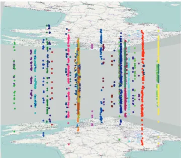
Not always starts and ends of trajectories correspond to takeoffs and landings. The radar observation data also contain parts of transit trajectories that just pass over France as well as flights going outside France and those coming to France from abroad. Real takeoffs and landings must be distilled from the available starts and ends of the recorded tracks. To extract the landings, we use the following query condition: the altitude is less than 1 km in the last 5 minutes of the trajectory. From each trajectory that has such points, we extract the last point as an m-event representing the landing (figure 7 right). In the second step of the analysis, we cluster the landing events by the spatial positions and directions (SD) using the thresholds of 1km and 30 degrees, respectively. The resulting SD-clusters are presented in the space-time cube in figure 8; the noise is excluded. The colors represent different clusters. The vertical alignments of points correspond to the airports where multiple landings took place during the day.
An interesting pattern can be observed in the area of Nice on the southeast of France. There are two SD-clusters of landings, yellow and green; their points make a column on the right in the cube. The green cluster appears as an intrusion inside the yellow one. This means that the landing direction changed in this area twice during the day, perhaps, due to a change of the wind (aircrafts take off and land facing the wind). The map fragment in figure 9 shows that the yellow cluster contains landings from the southwest and the green cluster landings from the northeast. The blue lines show the last ten minutes fragments of the respective trajectories and reflect the mandatory landing directions.
The observation of the direction changes gives us an idea that the temporal patterns of landings should be investigated not by airports only but by airports and landing directions. Therefore, we build 500-meter spatial buffers around the SD-clusters, as shown in figure 9. For an analysis by airports, irrespective of the directions, we would do a second stage of clustering (after excluding the noise) by only the spatial positions of the events and then build buffers around the resulting S-clusters.
Figure 8. The space-time cube shows the landing events clustered by spatial positions and directions.
Figure 9. The yellow and green dots represent two SD-clusters of landings in the airport of Nice. The time diagrams show the
dynamics of the landings from two directions.
In the third step of the analysis procedure, we aggregate the landing m-events in space by the buffers and in time by one-hour intervals. In the fourth step, we visualize the resulting time series by temporal diagrams positioned on the map display; two of them can be seen in the map fragment in figure 9. They show that the aircrafts landed in the airport of Nice from the southwest almost all time except for an interval in the middle of the day, when the landing direction changed to the opposite. The exact times and values are displayed when the mouse cursor points on an area.
Figure 10 presents the map with the temporal diagrams for the Paris region. We can see that the Orly airport and the northern runway of the Charles de Gaulle airport have clear peaks in the morning and in the evening. It is a typical pattern for airline hubs: short period of time, during which many fights arrive and take off, maximize the number of possible connections. The southern runway of the Charles de Gaulle airport is used with almost constant intensity during the day. The remaining airports are used much less intensively and mostly in the afternoon.
So far we have considered only the landings. To investigate the takeoffs, we repeat the procedure. To extract the takeoff events in the first step, we use the query condition that the altitude must be less than 1 km at the beginning of the trajectory. The remainder of the procedure is similar to that for the landings.
Figure 10. The time diagrams show the dynamics of landings in the airports of Paris.
To investigate the connections among the airports, we need to define the airport areas so that they include both the takeoff and the landing events. We join the sets of the takeoff and landing events, which have been previously filtered by removing the noise after the SD-clustering. Then we apply clustering by spatial positions, to unite the clusters of takeoffs and landings in different directions occurring at the same airports. We build spatial buffers around the S-clusters to obtain the airport areas. In the third step, we aggregate the trajectories by pairs of places (airport areas) and time intervals (1 hour length), as described in section 4.3. We use only those trajectories that have both takeoff and landing events. As a result, we obtain aggregate flows (vectors) with respective hourly time series and totals of flight counts.
To investigate the aggregates (step 4 of the procedure), we visualize the total counts on a flow map. The aggregate flows are shown by directed arrows with the widths proportional to the flight counts. By interactive filtering, we hide minor flows (less than 5 flights) and focus on the short-distance flows (below 100 km distance). We see that there are quite many flights connecting close airports, particularly, in Paris. As explained by a domain expert, a part of them are flights without passengers used for relocating aircrafts between big airports, such as Charles de Gaulle and Orly. Short-distance flows between small airports correspond to training and leisure flights of private pilots. Focusing on the long-distance flows (100 km and more) reveals a mostly radial connectivity scheme with a centre in Paris.
Figure 11. The distribution of the flights between the airports by hourly intervals. Highlighted are rows for the connections
Marseille-Paris (yellow) and Paris- Marseille (orange).
To investigate the temporal dynamics of the flows, we use the table display as shown in figure 11. The columns of the table correspond to the hourly time intervals and the rows to the flows.
The lengths of the colored bar segments in the cells are proportional to the flight counts for the respective flows and intervals. The colors correspond to the eight compass directions, as in figures 4-6. The table view is linked to the flow map. Thus, clicking on the vectors connecting Paris Orly and Marseille on the map, we get two rows highlighted. The yellow one corresponds to the northwestern direction, i.e., from Marseille to Paris, and the orange one to the opposite direction from Paris to Marseille. There are one or two flights from Marseille to Paris every hour in the intervals 07-14h and 15-18h and three flights per hour from 22h to midnight. The traffic in the opposite direction has a different profile: 3 flights per hour from midnight till 02h and several flights in the morning, at noon, and in the evening. The complementary link from the table view to the map can be used to locate flows with particular dynamics.
As compared to the example with the Milan cars data, this example demonstrates the extraction of two kinds of m-events (takeoffs and landings), another variant of two-stage clustering of events (SD-clustering followed by S-clustering), and the use of extracted places of interest for spatio-temporal aggregation of trajectories into flows between the places.
Validation of the findings. First, to assess the validity of the
extracted areas of takeoffs and landings, we compared them with the known positions of the airports and found that the areas include the airports. Furthermore, the areas have elongated shapes (figure 10) whose spatial orientations coincide with the orientations of the runways of the respective airports. Next, the results of data aggregation by the areas (i.e., counts of takeoffs, landings, and flights between airports) correspond very well to the common knowledge about the sizes and connectivity of the French cities and airports. The discovered patterns have been also checked and interpreted by a domain expert (one of the authors of the paper), who confirmed their plausibility.
7 CONCLUSION
We have developed a generic procedure for analyzing mobility data that is oriented to a class of problems where relevant places need to be determined from the mobility data in order to study place-related patterns of events and movements. We have described two examples of the use of the procedure; however, there are many other possible applications. Thus, sociologists investigating movement behaviors of people may look for places where people make long stops or where they meet and investigate the temporal patterns of the stops or meetings and the movements between the places. Biologists studying migration of animals may have similar interests. In analyzing maritime traffic, the procedure may allow an analyst to determine anchoring areas and areas of major turns and crossings, reconstruct the ship lanes, and investigate the dynamics of the traffic on these lanes. The procedure can also be applied to temporally sparse and irregular data such as mobile phone calls or positions of georeferenced photos published on photo sharing web sites.
In the future, we plan to integrate our tools for interactive visual analysis with the functionality of the moving object database.
ACKNOWLEDGMENT
The work has been partly supported by the DFG – Deutsche Forschungsgemeinschaft (German Research Foundation) within the research project ViAMoD – Visual Spatiotemporal Pattern Analysis of Movement and Event Data.
REFERENCES
[1] G.Andrienko, N.Andrienko, A general framework for using aggregation in visual exploration of movement data. The Cartographic Journal, 2010, 47 (1), pp. 22-40
[2] G.Andrienko, N.Andrienko, P.Bak, D.Keim, S.Kisilevich, S.Wrobel. A conceptual framework and taxonomy of techniques for analyzing movement. Journal of Visual Languages and Computing, 2011, 22(3), pp.213-232
[3] G.Andrienko, N.Andrienko, M.Heurich. An event-based conceptual model for context-aware movement analysis. International Journal Geographical Information Science, 2011, in press
[4] N.Andrienko, G.Andrienko. Spatial generalization and aggregation of massive movement data. IEEE Transactions on Visualization and Computer Graphics, 2011, 17(2), pp.205-219
[5] M.Ankerst, M.Breunig, H.-P.Kriegel, J.Sander. OPTICS: Ordering points to identify the clustering structure. In: ACM SIGMOD 1999, pp. 49–60.
[6] K. Beard, H. Deese, N.R. Pettigrew. A Framework for Visualization and Exploration of Events. Information Visualization, 7, 2008, pp. 133-151
[7] P.Buono, A.Aris, C.Plaisant, A.Khella, B. Shneiderman. Interactive Pattern Search in Time Series. In Proc. Conf. on Visualization and Data Analysis (VDA 2005), Washington DC, 2005, pp. 175-186 [8] F.Calabrese, F.Pereira, G.DiLorenzo, L.Liu, C.Ratti, The geography
of taste: analyzing cell-phone mobility and social events. In: Int. Conf. Pervasive Computing 2010, pp.22-37
[9] T.Crnovrsanin, C.Muelder, C.Correa, K.-L.Ma. Proximity-based visualization of movement trace data. In: VAST 2009, pp. 11-18 [10] S.Dodge, R.Weibel, E.Forootan, Revealing the physics of
movement: Comparing the similarity of movement characteristics of different types of moving objects. Computers, Environment and Urban Systems, 33(6), 2009, pp.419-434
[11] R.A.Enguehard, R.Devillers, O.Hoeber. Geovisualization of fishing vessel movement patterns using hybrid fractal/velocity signatures. In: GeoViz Hamburg 2011, online proceedings, http://www.geomatik-hamburg.de/geoviz/
[12] M.Ester, H.-P.Kriegel, J.Sander, X.Xu. A density-based algorithm for discovering clusters in large spatial databases with noise. In: ACM KDD 1996, pp. 226-231.
[13] A.Frank. Qualitative spatial reasoning about distances and directions in geographical space. Journal of Visual Languages and Computing, 1992, 3, pp. 343-371
[14] A.Fredrikson, C.North, C.Plaisant, B.Shneiderman. Temporal, geographical and categorical aggregations viewed through coordinated displays: a case study with highway incident data. In Proc. Workshop on New Paradigms in information Visualization and Manipulation. ACM, 1999, 26-34.
[15] F.Giannotti, M.Nanni, F.Pinelli, D.Pedreschi. Trajectory pattern mining. In: KDD 2007, pp. 330–339
[16] H.Guo, Z.Wang, B.Yu, H.Zhao, X.Yuan. TripVista: Triple perspective visual trajectory analytics and its application on microscopic traffic data at a road intersection. In: PacificVis 2011, pp. 163-170
[17] R.H.Güting, M.Schneider. Moving Objects Databases. Morgan Kaufmann, 2005
[18] T.Hägerstrand. What about people in regional science? Papers, Regional Science Association, 24, 1970, pp. 7-21.
[19] J.D.Hamilton. Time series analysis. Princeton University Press, 1994 [20] C.Hurter, B.Tissoires, S.Conversy. FromDaDy: Spreading aircraft
trajectories across views to support iterative queries. IEEE Transactions on Visualization and Computer Graphics, 15(6), 2009, pp. 1017-1024
[21] P.Kalnis, N.Mamoulis, S.Bakiras. On discovering moving clusters in spatio-temporal data. In: Advances in spatial and temporal databases 2005. LNCS 3633, 364-381
[22] J. Kim. Events as property exemplifications. In: M.Brand, D.Walton (eds.). Action Theory, Reidel, Dordrecht, 1976, pp. 159–177 [23] M.-J.Kraak, The space-time cube revisited from a geovisualization
perspective. In: Proc. 21st Int. Cartographic Conference, Durban, 2003, pp.1988-1995
[24] P.Laube, S.Imfeld, R.Weibel. Discovering relative motion patterns in groups of moving point objects. International Journal Geographic Information Science, 19(6), 2005, pp. 639–668
[25] P.A.Longley, M.F.Goodchild, D.J.Maguire, D.W.Rhind. Geographical Information Systems. Vol. 1: Principles and Technical Issues, Second Edition, John Wiley & Sons, New York, USA, 1999 [26] J.Macedo, C.Vangenot, W.Othman, N.Pelekis, E.Frentzos,
B.Kuijpers, I.Ntoutsi, S.Spaccapietra, Y.Theodoridis. Trajectory data models. In F.Giannotti & D.Pedreschi (eds.). Mobility, Data Mining and Privacy - Geographic Knowledge Discovery, Springer, Berlin, 2008, pp. 123-150
[27] J.F.Roddick, M.Spiliopoulou. A survey of temporal knowledge discovery paradigms and methods. IEEE Transactions on Knowledge and Data Engineering, 14(4), 2002, pp. 750-767
[28] R.Scheepens, N.Willems, H. van de Wetering, J.J. van Wijk. Interactive visualization of multivariate trajectory data with density maps. In: PacificVis 2011, pp. 147-154
[29] J.Wood, J.Dykes, A.Slingsby, Visualization of origins, destinations and flows with OD maps. The Cartographic Journal, 2010, 47(2), pp.117-129
[30] M.F.Worboys. Event-oriented approaches to geographic phenomena. International Journal of Geographic Information Science, 19(1), 2005, pp. 1-28
[31] Z.Yan, J.Macedo, C.Parent, S.Spaccapietra. Trajectory Ontologies and Queries. Transactions in GIS, 12(1), 2008, pp. 75 - 91