Modeling the 3D Milky Way using Machine Learning with Gaia and infrared surveys

HAL Id: tel-03155785

https://tel.archives-ouvertes.fr/tel-03155785

HAL is a multi-disciplinary open access archive for the deposit and dissemination of sci-entific research documents, whether they are pub-lished or not. The documents may come from teaching and research institutions in France or abroad, or from public or private research centers.

L’archive ouverte pluridisciplinaire HAL, est destinée au dépôt et à la diffusion de documents scientifiques de niveau recherche, publiés ou non, émanant des établissements d’enseignement et de recherche français ou étrangers, des laboratoires publics ou privés.

Modeling the 3D Milky Way using Machine Learning

with Gaia and infrared surveys

David Cornu

To cite this version:

David Cornu. Modeling the 3D Milky Way using Machine Learning with Gaia and infrared sur-veys. Astrophysics [astro-ph]. Université Bourgogne Franche-Comté, 2020. English. �NNT : 2020UBFCD034�. �tel-03155785�

pr´epar´ee `a l’Universit´e de Franche-Comt´e en vue de l’obtention du grade de

Docteur de l’Universit´e Bourgogne Franche-Comt´e

Modeling the 3D Milky Way

using Machine Learning

with Gaia and infrared surveys

Modélisation 3D de la Voie Lactée

par Machine Learning

avec les données infrarouges et Gaia

Specialité : Astrophysique soutenue par

David Cornu

à Besançon, le 29 September 2020

Thèse supervisée par: Annie Robin et Julien Montillaud

Composition du jury :

Rosine, Lallement Directrice de recherche - Université PSL (GEPI) Rapportrice Luis M., Sarro Baro Professeur associé - UNED (AI Dept.) Rapporteur Anne S.M., Buckner Chargée de recherche - Université de Exeter Examinatrice Douglas J., Marshall Maître de conférences - Université Toulouse III, P. Sabatier Examinateur Raphael, Couturier Professeur - IUT Belfort-Montbéliard President Sylvain, Bontemps Directeur de recherche - Université de Bordeaux Examinateur Annie, Robin Directrice de recherche - Université de Franche-Comté Directrice de thèse Julien, Montillaud Maître de conférences - Université de Franche-Comté Codirecteur de thèse

Ecole Doctorale : Carnot-Pasteur, ED 553

Laboratoire : Institut UTINAM, Observatoire de Besançon UMR CNRS 6213, Besançon, France

Cette thèse a été co-financée par le Centre National d’études Spatiales (CNES) et par la région Bourgogne Franche-Comté. Le CNES, dans son rôle d’employeur, nous a assuré son soutien administratif et financier à plusieurs reprises. Le laboratoire UTI-NAM et l’Observatoire des Sciences de l’Univers THETA de l’université de Bourgogne Franche-Comté ont été les lieux d’accueil quotidien pour nos travaux, et nous tenons à remercier les différentes instances (laboratoire, équipe, OSU) qui nous ont soutenu financièrement et administrativement à de nombreuses reprises. Nos remerciements se portent également vers le Mésocentre de l’Université de Franche-Comté et le Mas-ter CompuPhys qui nous ont permis d’accéder à d’importantes ressources de calculs indispensables au travail réalisé. Enfin, nous remercions différents projets et collabo-rations auxquels nous avons eu la chance de participer : le projet GALETTE financé par PCMI, le projet Besançon-Budapest-Collaboration (BBC), le groupe Galactic Cold Cores (GCC), et l’International Space Science Institute (ISSI) qui a hébergé un groupe de travail autour du modèle de la Galaxie de Besançon.

Remerciements informels

Tout d’abord je tiens profondément à remercier Julien Montillaud, envers qui toute ma gratitude ne saurait s’exprimer en seulement quelques lignes. Merci à Julien d’abord pour sa disponibilité, sa bienveillance, et surtout son éternelle patience, dans l’encadrement de cette thèse. Sa motivation débordante et communicative fut un véritable moteur pour moi au quotidien. Merci aussi pour tout ce qu’il m’a appris, tant sur le plan scientifique qu’humain. Merci de m’avoir aidé à donner le meilleur de moi-même et de m’avoir poussé à élargir mes compétences et intérêts. Ce serait un immense plaisir pour moi que nous puissions continuer à travailler ensemble dans les années à venir.

Merci également à Annie Robin pour son encadrement. Annie a su me faire profiter de sa très grande expérience et a toujours été disponible pour m’aider à avancer dans mes travaux. Merci notamment pour son regard critique très pertinent qui nous a per-mis de souvent dépasser nos objectifs et d’étendre nos champs d’expertise. Je tiens à chaleureusement remercier les autres collègues (passés ou actuels) du bâtiment des hor-loges : Jean-Baptiste, Nadège, Céline et Guillaume. Merci à chacun d’entre eux pour leur regard scientifique sur nos progrès, pour leurs suggestions de travaux, et pour tous leurs conseils qui m’ont permis de progresser dans de nombreux domaines. J’espère avoir la chance de pouvoir continuer à travailler avec eux, et que nous aurons l’occasion de concrétiser beaucoup des idées que nous avons pu avoir ensemble. Merci également à eux pour les moments de partages, au laboratoire ou en mission, et d’une manière plus générale pour m’avoir intégré aussi chaleureusement à l’équipe.

Merci à tous les membres de l’observatoire et du laboratoire UTINAM pour leur ac-cueil. Je pense en particulier à tous mes collègues avec qui j’ai partagé "journal club", réunions, séminaires, mais aussi de nombreux moments de convivialité. J’adresse tous mes voeux de réussite à mes collègues doctorants et jeunes docteurs qui ont été une incroyable source de soutien et d’échange. Merci à tous mes collègues pour la place qu’ils m’ont laissée prendre dans ce groupe; je ne crois pas retrouver facilement une ambiance aussi bienveillante au sein d’une équipe.

Special thanks:

I want to warmly thank all the jury members for their clear interest in my work and for all their comments and suggestions that helped me to improve the quality of the present manuscript and to consider new research ideas. I also want to express a great thank you to Anne Buckner for her help to improve the manuscript language quality.

Abstract

Large-scale structure in the Milky Way (MW) is, observationally, not well constrained. Studying the morphology of other galaxies is straightforward but the observation of our home galaxy is made difficult by our internal viewpoint. Stellar confusion and screening by interstel-lar matter are strong observational limitations to assess the underlying 3D structure of the MW. At the same time, very large-scale astronomical surveys are made available and are expected to allow new studies to overcome the previous limitations. The Gaia survey that contains around 1.6 billion star distances is the new flagship of MW structure and stellar population analyses, and can be combined with other large-scale infrared (IR) surveys to provide unprecedented long distance measurements inside the Galactic Plane. Concurrently, the past two decades have seen an explosion of the use of Machine Learning (ML) methods that are also increasingly employed in astronomy. With these methods it is possible to automate complex problem solving and e ffi-cient extraction of statistical information from very large datasets.

In the present work we first describe our construction of a ML classifier to improve a widely adopted classification scheme for Young Stellar Object (YSO) candidates. Born in dense inter-stellar environments, these young stars have not yet had time to significantly move away from their formation site and therefore can be used as a probe of the densest structures in the interstel-lar medium. The combination of YSO identification and Gaia distance measurements enables the reconstruction of dense cloud structures in 3D. Our ML classifier is based on Artificial Neu-ral Networks (ANN) and uses IR data from the Spitzer Space Telescope to reconstruct the YSO classification automatically from given examples. We extensively explore dataset constructions and the effect of imbalanced classes in order to optimize our ANN prediction and to provide reliable estimates of its accuracy for each class. Our method is suitable for large-scale YSO can-didate identification and provides a membership probability for each object. This probability can be used to select the most reliable objects for subsequent applications like cloud structure reconstruction.

In the second part, we present a new method for reconstructing the 3D extinction distribution of the MW and that is based on Convolutional Neural Networks (CNN). With this approach it is possible to efficiently predict individual line of sight extinction profiles using IR data from the 2MASS survey. The CNN is trained using a large-scale Galactic model, the Besançon Galaxy Model, and learns to infer the extinction distance distribution by comparing results of the model with observed data. This method has been employed to reconstruct a large Galactic Plane portion toward the Carina arm and has demonstrated competitive predictions with other state-of-the-art 3D extinction maps. Our results are noticeably predicting spatially coherent structures and significantly reduced artifacts that are frequent in maps using similar datasets. We show that this method is able to resolve distant structures up to 10 kpc with a formal resolution of 100 pc. Our CNN was found to be capable of combining 2MASS and Gaia datasets without the necessity of a cross match. This allows the network to use relevant information from each dataset depending on the distance in an automated fashion. The results from this combined prediction are encouraging and open the possibility for future full Galactic Plane prediction using a larger combination of various datasets.

Titre en français : Modélisation de la Voie Lactée en 3D par machine

learn-ing avec les données infrarouges et Gaia

La structure à grande échelle de la Voie-Lactée (VL) n’est actuellement toujours pas par-faitement contrainte. Contrairement aux autres galaxies, il est difficile d’observer directement sa structure du fait de notre appartenance à celle-ci. La confusion entre les étoiles et l’occultation de la lumière par le milieu interstellaire (MIS) sont les principales sources de difficulté qui em-pêchent la reconstruction de la structure sous-jacente de la VL. Par ailleurs, de plus en plus de relevés astronomiques de grande ampleur sont disponibles et permettent de surmonter ces difficultés. Le relevé Gaia et ses 1.6 milliards mesures de distances aux étoiles est le nouvel outil de prédilection pour l’étude de la structure de la VL et l’analyse des populations stel-laires. Ces nouvelles données peuvent être combinées avec d’autres grands relevés infrarouges (IR) afin d’effectuer des mesures à des distances jusque-là inégalées. Par ailleurs, le nombre d’applications reposant sur des méthodes d’apprentissage machine (AM) s’est envolé ces vingt dernières années et celles-ci sont de plus en plus employées en astronomie. Ces méthodes sont capables d’automatiser la résolution de problèmes complexes ou encore d’extraire efficacement des statistiques sur de grands jeux de données.

Dans cette étude, nous commençons par décrire la construction d’un outil de classifica-tion par AM utilisé pour améliorer les méthodes classiques de classificaclassifica-tion des Jeunes Objets Stellaires (JOS). Comme les étoiles naissent dans un environnement interstellaire dense, il est possible d’utiliser les plus jeunes d’entre elles, qui n’ont pas encore eu le temps de s’éloigner de leur lieux de formation, afin d’identifier les structures denses du MIS. La combinaison des JOS et des distances mesurées par Gaia permet alors de reconstruire la structure 3D des nuages denses. Notre méthode de classification par AM est basée sur les réseaux de neurones artificiels et se sert des données du télescope spatial Spitzer pour reconstruire automatiquement la classi-fication des JOS sur la base d’une liste d’exemples. Nous détaillons la construction des jeux de données associés ainsi que l’effet du déséquilibre entre les classes, ce qui permet d’optimiser les prédictions du réseau et d’estimer la précision associée. Cette méthode est capable d’identifier des JOS dans de très grands relevés tout en fournissant une probabilité d’appartenance pour chacun des objets testés. Celle-ci peut alors être utilisée pour retenir les objets les plus fiables afin de reconstruire la structure des nuages.

Dans une seconde partie, nous présentons une méthode permettant de reconstruire la dis-tribution 3D de l’extinction dans la VL et reposant sur des réseaux de neurones convolutifs. Cette approche permet de prédire des profils d’extinction sur la base de données IR provenant du relevé 2MASS. Ce réseau est entraîné à l’aide du modèle de la Galaxie de Besançon afin de reproduire la distribution en distance de l’extinction à grande échelle en s’appuyant sur la comparaison entre le modèle et les données observées. Nous avons ainsi reconstruit une grande portion du plan Galactique dans la région du bras de la Carène, et avons montré que notre pré-diction est compétitive avec d’autres cartes d’extinction 3D qui font référence. Nos résultats sont notamment capables de prédire des structures spatialement cohérentes, et parviennent à réduire les artefacts fréquents dits “doigts de Dieu”. Cette méthode est parvenue à résoudre des structures distantes jusqu’à 10 kpc avec une résolution formelle de 100 pc. Notre réseau est également capable de combiner les données 2MASS et Gaia sans avoir recours à une iden-tification croisée. Cela permet d’utiliser automatiquement le jeu de données le plus pertinent en fonction de la distance. Les résultats de cette prédiction combinée sont encourageants et ouvrent la voie à de nouvelles reconstructions du plan Galactique en combinant davantage de jeux de données.

Abstract

Résumé en Français

I

Context

1

1 Milky Way 3D structure 5

1.1 Review of useful properties of the Milky Way . . . 5

1.1.1 The only galaxy that can be observed from the inside . . . 5

1.1.2 Expected structural information . . . 8

1.2 The interstellar medium . . . 9

1.2.1 The bridge between stellar population and interstellar medium . . . . 9

1.2.2 Interstellar medium extinction and emission . . . 10

1.3 Observational constraints on the Milky Way structure . . . 14

2 The rise of AI in the current Big Data era 18 2.1 Proliferation of data and meta-data . . . 18

2.2 Artificial intelligence, a not-so-modern tool . . . 19

2.2.1 Beginnings of AI . . . 19

2.2.2 End of 20th century difficulties and successes . . . 19

2.2.3 The new golden age of AI . . . 20

2.2.4 Astronomical uses of AI . . . 20

2.3 Astronomical Big Data scale surveys . . . 21

2.3.1 Previous large surveys . . . 21

2.3.2 A new order of magnitude with PanSTARRS and Gaia . . . 22

2.3.3 The historical challenge of SKA and following surveys . . . 22

II

Young Stellar Objects classification

25

3.2 YSO candidates identification. . . 29

3.3 Machine Learning motivation and previous attempts . . . 31

3.4 Objective and organization . . . 32

4 Classical Artificial Neural Networks 33 4.1 Attempt of ML definition . . . 34

4.1.1 "Animal" learning and "Machine" Learning . . . 34

4.1.2 Types of artificial learning . . . 35

4.1.3 Broad application range and profusion of algorithms . . . 36

4.1.4 Toolboxes against home-made code . . . 36

4.2 Artificial Neuron . . . 40

4.2.1 Context and generalities . . . 40

4.2.2 Mathematical model . . . 41

4.2.3 Supervised learning of a neuron . . . 42

4.4 Perceptron algorithm: linear combination . . . 44

4.5 Multi Layer Perceptron : universal approximation . . . 46

4.5.1 Non linear activation function and neural layers stacking . . . 46

4.5.2 Supervised network learning using backpropagation . . . 48

4.6 Limits of the model . . . 50

4.7 Neural network parameters . . . 51

4.7.1 Network depth and dataset size . . . 51

4.7.2 Learning rate . . . 52

4.7.3 Weight initialization . . . 54

4.7.4 Input data normalization . . . 55

4.7.5 Weight decay . . . 55

4.7.6 Monitor overtraining . . . 56

4.7.7 Shuffle and gradient descent schemes . . . 58

4.7.8 Momentum conservation . . . 59

4.8 Matrix formalism and GPU programming . . . 60

4.8.1 Hardware considerations for matrix operations . . . 60

4.8.2 Artificial Neural networks as matrix operations . . . 61

4.8.3 GPUs variety . . . 62

4.8.4 Insights on GPU programming . . . 65

4.9 The specificities of classification . . . 67

4.9.1 Probabilistic class prediction . . . 67

4.9.2 The confusion matrix . . . 69

4.9.3 Class balancing and observational proportions . . . 70

4.10 Simple examples . . . 73

4.10.1 Regression . . . 73

4.10.2 Classification . . . 76

5 Automatic identification of YSOs in infrared surveys 79 5.1 Problem description and class definition . . . 79

5.2 Labeled datasets in Orion, NGC 2264, 1 kpc and combinations . . . 82

5.3 Construction of the test, valid and train dataset . . . 87

5.4 Network architecture and parameters . . . 90

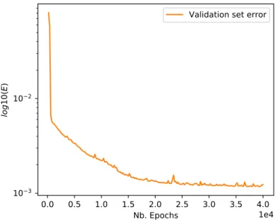
5.5 Convergence criteria . . . 93

6 Subsequent application to multiple star-forming regions 94 6.1 First training on one specific region: the Orion molecular cloud . . . 95

6.1.1 Hyper-parameter and training proportion evaluation . . . 95

6.1.2 Main result . . . 96

6.1.3 Test on a balanced dataset . . . 96

6.1.4 Prediction stability . . . 97

6.1.5 Detailed sub-classes distribution . . . 97

6.1.6 Full dataset result . . . 98

6.2 Effect of the selected region: training using NGC 2264 . . . 99

6.2.1 Main result . . . 99

6.2.2 Small dataset issues . . . 100

6.2.3 Prediction stability . . . 100

6.3.2 O-N main result . . . 103

6.3.3 Detailed feature space analysis for O-N . . . 104

6.3.4 N-O main result . . . 105

6.3.5 Detailed feature space analysis for N-O . . . 106

6.4 Improving diversity: combined training . . . 107

6.4.1 Hyper-parameter and training proportion changes . . . 108

6.4.2 Main result . . . 108

6.4.3 Generalization capacity evaluation . . . 109

6.4.4 Full dataset result and analysis of rare sub-classes prediction . . . 110

6.5 Further increase in diversity and dataset size: nearby regions (< 1kpc) . . . . 111

6.5.1 Hyper-parameter and training proportion changes . . . 111

6.5.2 Main result . . . 111

6.5.3 More detailed analysis . . . 112

6.5.4 Full dataset result . . . 113

6.5.5 Misclassified objects distribution . . . 113

6.5.6 Forward of the trained network on Orion and NGC 2264 . . . 114

6.6 Orion and NGC 2264 YSO candidates distribution maps . . . 118

7 Probabilistic prediction contribution to the analysis 121 7.1 Interpretation of the membership probability . . . 122

7.2 Graphical analysis of the membership probability . . . 127

8 3D cloud reconstruction using cross-match with Gaia 134 8.1 Orion A distance and 3D information . . . 134

8.2 Distances to Orion B sub-regions . . . 139

8.3 NGC 2264 distance and 3D information . . . 141

9 Additional discussion and further improvements 143 9.1 Identified limitations to our results . . . 143

9.2 MIPS 24 micron band effect on the results . . . 144

9.3 Usage of Spitzer colors instead of bands . . . 144

9.4 Method discussion. . . 145

9.5 Conclusion and perspectives . . . 146

III

Reconstruction of the 3D interstellar extinction of the MW

149

10.2 Per line of sight approach . . . 155

10.3 The Besançon Galaxy Model . . . 158

10.4 Mesuring extinction using the BGM . . . 159

10.5 Using Machine Learning for this task . . . 160

11 Convolutional Neural Networks 162

11.1 The image processing impulse . . . 162

11.1.1 Spatially coherent information . . . 162

11.1.2 Information redundancy: pattern recognition. . . 165

11.1.3 Convolution filter . . . 166

11.1.4 Convolutional layer . . . 168

11.1.5 A simpler activation function : the rectified linear unit. . . 172

11.1.6 Stacking Convolutional layers . . . 174

11.1.7 Pooling layer . . . 175

11.1.8 Learning the convolutional filters. . . 176

11.2 Convolutional networks parameters . . . 181

11.2.1 Convolutional Neural Network architectures . . . 181

11.2.2 Weight initialization and bias value. . . 184

11.2.3 Additional regularization: Dropout and momentum . . . 185

11.2.4 Implications for GPU formalism . . . 186

11.2.5 Example of a classical image classification. . . 189

11.3 Use of the dropout to estimate the uncertainty in a regression case . . . 191

12 Extinction profile reconstruction for one line of sight 193 12.1 Construction of a simulated 2MASS CMD using the BGM . . . 193

12.1.1 Choice of BGM representation and observed quantity . . . 193

12.1.2 Reproducing realistic observations: uncertainty and magnitude cuts . 196 12.1.3 Simple extinction effect on the diagram . . . 198

12.2 Creating realistic extinction profiles for training . . . 200

12.2.1 Gaussian Random Fields . . . 200

12.2.2 GRF generated profile . . . 201

12.2.3 Profile star count limit and magnitude cap . . . 202

12.3 Tuning the method . . . 204

12.3.1 Input and output dimensions . . . 204

12.3.2 Network architecture . . . 205

12.3.3 Network hyperparameters . . . 206

12.3.4 Computational aspects . . . 208

13 2MASS only extinction maps 209 13.1 Training with one line of sight . . . 209

13.1.1 Network training and test set prediction . . . 209

13.1.2 Generalizing over a Galactic Place portion . . . 210

13.1.3 Integrated view of the plane of the sky . . . 212

13.1.4 Face-on view . . . 214

13.2 Combination of several lines of sight in the same training . . . 218

13.2.1 Sampling in galactic longitude . . . 218

13.2.2 Multiple line of sights in a single training . . . 218

13.2.3 Dataset construction, architecture effect and training . . . 219

13.2.4 Map results . . . 221

13.2.5 Effect of the galactic latitude . . . 226

13.3 Comparison with other 3D extinction maps . . . 228

14.2 Training with one line of sight . . . 238

14.3 Combined sampled training . . . 240

15 Method discussion and conclusion 244 15.1 Dataset construction limits and improvements . . . 244

15.1.1 Magnitude cuts and uncertainty issues . . . 244

15.1.2 Modular Zlimvalue . . . 244

15.1.3 Construction of realistic profiles . . . 245

15.1.4 The "perfect BGM model" assumption . . . 246

15.2 CNN method discussion. . . 246

15.3 Conclusion and perspectives . . . 247

16 General conclusion 248

Appendix

250

A.2 CIANNA objects . . . 255

A.3 Description of the layers . . . 256

A.3.1 Dense layer . . . 256

A.3.2 Pooling layer . . . 256

A.3.3 Convolutional layer . . . 257

A.4 Im2col function . . . 258

A.5 Other important functions . . . 260

A.6 Python and C interfaces . . . 260

A.7 Performance comparison . . . 264

A.8 Future improvements . . . 265

List of Figures

268

List of Tables

270

1 Milky Way 3D structure 5

1.1 Review of useful properties of the Milky Way . . . 5

1.1.1 The only galaxy that can be observed from the inside . . . 5

1.1.2 Expected structural information . . . 8

1.2 The interstellar medium . . . 9

1.2.1 The bridge between stellar population and interstellar medium . . . 9

1.2.2 Interstellar medium extinction and emission . . . 10

1.3 Observational constraints on the Milky Way structure . . . 14

2 The rise of AI in the current Big Data era 18 2.1 Proliferation of data and meta-data . . . 18

2.2 Artificial intelligence, a not-so-modern tool . . . 19

2.2.1 Beginnings of AI . . . 19

2.2.2 End of 20th century difficulties and successes . . . 19

2.2.3 The new golden age of AI . . . 20

2.2.4 Astronomical uses of AI . . . 20

2.3 Astronomical Big Data scale surveys . . . 21

2.3.1 Previous large surveys . . . 21

2.3.2 A new order of magnitude with PanSTARRS and Gaia . . . 22

1

Milky Way 3D structure

In this section we introduce astronomical knowledge that is relevant to understand the context of the present study. We noticeably describe the presently admitted view of our galaxy the Milky Way along with a few order of magnitude for the useful astronomical objects and quantity. We describe the expected structural information of the Milky Way and highlight its support from observational constrains. In a second time we expose some properties of the interstellar medium, summarizing its link with the stars in the galaxy. We end by describing the extinction from the ISM and its link with the structural information of the Milky Way.

1.1 Review of useful properties of the Milky Way . . . 5

1.1.1 The only galaxy that can be observed from the inside . . . 5

1.1.2 Expected structural information . . . 8

1.2 The interstellar medium . . . 9

1.2.1 The bridge between stellar population and interstellar medium . . . 9

1.2.2 Interstellar medium extinction and emission . . . 10

1.3 Observational constraints on the Milky Way structure . . . 14

1.1

Review of useful properties of the Milky Way

1.1.1 The only galaxy that can be observed from the inside

A natural beginning of a work on the Milky Way galaxy structure would be to define what a galaxy exactly is. Still, the presently accepted definition is not that old. In the 1920’s, two visions of our place in the universe was opposed in what was latter called the "Great debate". The argument was mostly opposing the two astronomers Harlow Shapley and Heber D. Curtis. The former defended the thesis that every astronomical object observed and especially what they called distant spiral nebulae was part of our Milky Way, so these nebulae must be close and small. The second one in contrast, argued that these objects were very distant and very large and were likely to be external galaxies that look very alike our own Milky Way of billions of stars. They published a common paper containing two parts where each of them exposed their arguments and that was titled The Scale of the Universe Shapley & Curtis (1921). The difference in physical scale between the two points of view was of several orders of magnitude, illustrating how much was remaining to understand just 100 years ago.

A few years later another famous astronomer, Edwin Hubble, published a paper that esti-mated the distance of these spiral nebulae based on the known absolute magnitude of Cepheid variable stars (Hubble 1926). The distances he found are today known to be significantly un-derestimated, still they were already large enough distances to support the thesis defended by Curtis that these nebulae were very large, very massive, distant structures. Later, he published the study that gave birth to the Hubble law and that correlates the distance and radial velocity of other galaxies with their reddening (Hubble 1929), which is now understood as a cosmological effect of the universe expansion. The known scale of the universe had drastically changed in a few years.

We do not aim at making an historical overview of the astronomical knowledge about galax-ies here, but this story illustrates the fact that knowing the physical scale and boundary of our own galaxy was a tricky question at this time (e.gKapteyn 1922). The currently accepted view of a galaxy is a system of stars, dust, gas, and dark matter that is gravitationally bound. Their

1.1 Review of useful properties of the Milky Way

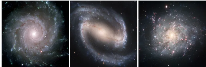
Figure 1.1: Examples of spiral galaxies that present different detailed morphology. From left to right,NGC 628 (M74), a grand design spiral galaxy (SA(s)c) observed by the 8.1-meter North Telescope of the Gemini Observatory ,NGC 1300a barred spiral galaxy (SB(s)bc) observed by the Hubble space telescope, andNGC 7793a flocculent galaxy (SA(s)d) observed by the ESO Very Large Telescope (VLT).

size can vary from a few kpc to more than 100 kpc and their mass estimates are mostly between 105 _{and 10}13 _M

 based on rotation curves. Galaxies have many different forms, as described by Hubble (1936) and successively refined in De Vaucouleurs (1959); De Vaucouleurs et al.

(1991); Lintott et al.(2008, ,...), and the most noticeable ones for the present study are spiral galaxies. Figure1.1shows three typical observed galaxies of this type (NGC 628 - M74, NGC 1300 and NGC 7793) with a face-on view of their plane spanned by spiral-shaped arms that start from the bulge and coil out progressively. This figure also illustrates the large variety of possible spiral structures, with a variable number of arms and a center that can be a roughly-spherical bulge or in other cases an elongated bar. There is also an opposition between two views of galaxy structures: (i) the grand-design view that corresponds to very well resolved narrow spiral arms at large scale which could be the case of M74 in the left frame, and (ii) the flocculent view of more sub-structured galaxies with sub-arms, arm discontinuities, bridges between them, and that does not always follow the expected spiral shape as illustrated in the left frame with NGC 7793. Most of the star formation is believed to occur in the arms (Solomon & Rivolo 1989;Salim & Rich 2010) even if the galaxy mass is mostly evenly sprayed over the whole disk (McMillan 2017). This disk is rotating around the central bulge or bar region that hosts a supermassive black hole for most galaxies (Heckman & Best 2014) and concentrates an important fraction of its mass. This global structure of a galaxy is expected to come from their formation process that started quickly in the early stages of the universe and that is still going on today (Freeman & Bland-Hawthorn 2002). While there are multiple views on which process dominates the galaxies formation, it is mostly accepted that there is a gravitational collapse of matter at large scale (Cooper et al. 2010) and that the rotating accreted matter speeds up with the decrease in the structure size creating a flatten disk shape structure (Brook et al. 2004). In-terestingly, there are still to this day a lot of unknowns about our home galaxy structure, size, mass, detailed 3D distribution of star, etc (Bland-Hawthorn & Gerhard 2016). We are presently in an uncomfortable situation, where we know more about other galaxies large-scale structures that are far way from us, than about our own galaxy structure. This is due exactly to the fact the we are part of this galaxy. While it is possible to see other galaxies face-on, our own galaxy obscures itself since we are inside the galactic plane and relatively far away from the center.

Figure 1.2: Most common artistic face-on view of the Milky Way that illustrates the expected Milky Way bulge and arms. FromHurt(2008).

Figure 1.3: Gaia DR2 view of the Milky Way in the plane of the sky. The image is not a photograph, but a map of the 1.6 billion star brightness in the survey. The image is encoded using the Gaia magnitude bands following, Red: GRP, Green: G and Blue: GBP. From Gaia

1.1 Review of useful properties of the Milky Way

The most used Milky Way representation is the one presented in Figure 1.2 from Hurt

(2008). Despite the fact that this view was constructed based on some observations and on strong theoretical knowledge from the observation of other galaxy structures, it remains mostly an artistic representation that is strongly underconstrained. This view conveys the idea that this is the present state-of-the-art astronomical knowledge of our galaxy structure, even though only sparse and heterogeneous observational evidences are available to this day. What can truly be observed from our standpoint looks like the Figure1.3that contains all the observed stars from the Gaia DR2 mission that we will describe in Section2.3.2. This view illustrates the difficulty caused by our position inside the Milky Way. A great thought experiment that we got from a colleague, is to picture the Milky Way as an expanded forest. Once inside, it is possible to see through a tenth of meter depending on the tree density, but at some point the accumulation of trees and vegetation with the distance makes the view opaque. It is therefore impossible to properly assess the size of the forest from the inside. In this view the trees correspond to the stars and the most diffuse vegetation to the gas and dust distributed in the Milky Way disk. From this it is more clear why it is difficult to reconstruct the Milky Way large-scale structure. Still, it remains a favored position to study the interstellar medium and the stars themselves.

1.1.2 Expected structural information

In the present section we summarize some of the Milky Way (hereafter MW) properties based on the present knowledge (mostly followingBland-Hawthorn & Gerhard 2016) in order to con-textualize the present study. The MW is a rather evolved galaxy that has a decreasing star formation and does not present traces of important merger history. It is usually classified as a Spiral Sb-Sbc galaxy, and most of the representations account for 4 spiral arms. Most mea-surements predict a stellar mass around 5 × 1010Mand total galactic mass from the large dark matter halo around ∼ 1.5 × 1012_M

. The stellar disk radius is often estimated at 10 kpc and is often separated in two stellar populations, one from a thin disk with a scale height estimated around zt ' 300 pc and an older one from a thick disk with a scale height zT _{' 900pc depending} on the study, both presenting a flaring, i.e. an increase in height scale with galactic radius. The Sun position is estimated at around 8 kpc from the center of the MW and roughly positioned at an elevation of z0 ' 25pc. At the center of the MW is a super massive black hole named Sagit-tarius A∗_{for which the mass is estimated at approximately 4 × 10}6_M

, around which a nuclear star cluster is found. They are themselves embedded in an X-shaped (or peanut-shaped) bulge structure that is ∼ 3 kpc long and with a scale height of ∼ 0.5 kpc (Robin et al. 2012b). There is then a “long bar” or “thin bar” region that extend after the bulge up to a 5 kpc half-length (Wegg et al. 2015) but with a quickly decreasing height profile with a mean 180 pc scale height.

The previous elements are considered to be the main components of the Milky Way and provide an accurate global representation based on relatively well-constrained observations. Then the arm structures are more difficult to constrain since they are mostly defined by their higher luminosity or peculiar stellar population and do not represent strong star over-density in stellar mass (Salim & Rich 2010;McMillan 2017). They are proposed to be self-propagated compression waves created by the differential rotation of the galaxy. In this model an arm is a spiral-shaped local compression that triggers star formation and propagates through the galactic plane, which explains that the star velocities do not match those of the arms (Shu 2016). This process triggers intense star formation episodes, where massive stars are more likely to form than in other regions of the galaxy, highlighting the spiral arm shape. Since these massive stars have a very short life-time, they are gone soon after the passage of the wave, inducing rela-tively narrow spiral arm structures. As we will expose in Section1.2.1, stars form from dense

cloud compression, therefore the arm structures are also traced by dense interstellar environ-ment which will be at the center of the present study. Overall, in contrast with what Figure1.2

support, the MW arms are mostly under relatively weak observational constrains at these day which is discussed in Section1.3

1.2

The interstellar medium

1.2.1 The bridge between stellar population and interstellar medium

The main components of galaxies are stars, but they evolve in a more diffuse matter environ-ment, the Inter Stellar Medium (ISM), to which they are bound through a complex interplay. Mainly, the ISM is a mixture of gas and dust with a huge diversity of states and detailed compo-sition. Overall the mass of the ISM is divided as 70.4% Hydrogen, 28.1% Helium, and 1.5% of heavier atoms, almost all of it being in a gas state with less than 1% of the mass of this matter being in the form of solid dust grains (Ferrière 2001). This matter is distributed very heteroge-neously in the galactic environment, from very warm diffuse (TK > 105K and n < 0.01 cm−3) and almost transparent large-scale structures to very dense and cold structures (TK ∼ 10 K and n> 103_cm−3_{) at much smaller scales with a continuum of structures between the two, including} for example interstellar molecular filaments.

The ISM evolution is determined by the complex interplay between the magneto-hydrodynamics laws, which describe how the gas flows in the galaxy, gravity and self-gravity, which contribute to shaping and compressing the gas at all scales, as well as a number of processes related to stellar evolution, like the propagation of supernova shock waves, the gas heating by photoelec-tric effect on dust grains or gas ionization by stellar ultra-violet (UV) flux. The ISM represents a significant portion of the mass of the Milky way, equivalent to around 10 to 15% of the to-tal stellar mass. This is known to be the matter from which stars form as explained in detail, for example, byMcKee & Ostriker(2007), Kennicutt & Evans(2012), and references therein, and described briefly here. From the proportions reported above, it is visible that the MW has already converted most of its gas into stars. Under the combined effects of dynamics and grav-ity the interstellar medium will contract hierarchically creating dense clouds. At some point they will become optically thick and their inside will get cooler by preventing the ambient UV light from stars to penetrate the cloud deeply. The low temperatures enable a complex chem-istry catalyzed by dust grains that allows the creation of larger molecules and lets dust grain themselves grow in size, which changes the optical properties of the densest structures. The definition threshold of a dense cloud is a tricky question that is often solved using a certain amount of CO emission or by the dust reddening amount that is much higher in dense clouds. If the cloud is massive enough so that gravity is stronger than the gas support (kinetic energy, turbulence, magnetic field), it will collapse gravitationally, starting the formation of a protostar. It ultimately leads to the formation of a star that is supported by nuclear fusion in its core, i.e. a sequence star. The steps of star-formation, from the gravitational collapse to the main-sequence star are described where they are useful in Section3.1.

The important point here is that stars are formed through the collapse of the dense interstel-lar medium. Once formed, the stars will progressively get away from their original structure, so that identifying Young Stellar Objects (YSO) that did not have time to move too much is a suit-able way to reconstruct large-scale dense-cloud structures that are massive enough to form stars (Sect. 8). A large part of the present study, namely the part II, is dedicated to the construction of a YSO identification method that is a prerequisite of the previous approach.

1.2 The interstellar medium

More generally the link between the stars and the ISM is not one-sided since there are a lot of feedback from the stars on the ISM, of which we give some examples. First the star light warms and ionizes the ISM but also breaks any complex molecule or even evaporate dust grains. In addition, any element other than hydrogen and helium originate from the stellar nu-cleosynthesis and are dispersed after the star end of life. The supernova explosions that ends the life of massive stars (M > 8M) play a major and ambiguous role in the ISM evolution. This phenomenon is known to inject a very significant mechanical energy to the ISM, which can blow away dense structures and enrich it with new elements that are only formed during such energetic events. It can also have the opposite effect and induce compression waves on the ISM, leading to triggered star formation (e.gPadoan et al. 2017).

At large scales, the ISM is shaped by the global dynamic of the Milky Way. Indeed larger ISM structure have been observed to follow the spiral arms in other galaxies (e.g Elmegreen et al. 2003) and in simulations (Bournaud & Combes 2002) with the more local structures getting their energy mostly from gravitational instabilities from the spiral arms that drive the turbulent regime and by inward mass accretion (Bournaud et al. 2010). This explains why the large-scale structures of galaxies can be traced using the distribution of the dense ISM. Still, smaller scales of the local ISM distribution are made more complex by various feedback effects like supernovae (Hennebelle & Iffrig 2014) that are important to account for the flocculent substructures in galaxies, as it is illustrated by the Figure 1.3 to explain higher latitude dense clouds, or again in the right frame of Figure1.1.

1.2.2 Interstellar medium extinction and emission

While the ISM can be studied through its several interactions with stars, it is possible to perform more direct detection of the ISM structures. The first observable effect, even by the human eye, is the screening effect of the background stars by the interstellar clouds as can be observed in the Milky Way plane in Figure 1.3. This is due to an effect of the ISM called extinction and that sums two physical effects: the absorption and the scattering of the light by the matter in the light path. For astronomical considerations this effect induced predominantly by interstellar dust grains (Draine 2003, and reference therein). This extinction is usually characterized by the quantity Aλ: Aλ = 2.5 log F0 λ Fλ ! (1.1)

where F0 _{is the luminosity flux before the clouds, F is the flux after the cloud and A}

λ is the total extinction at the wavelength λ. An important point is that all these quantities depend of the wavelength of the light. This is due to the dependence of scattering to the ratio between the wavelength and the grain size, while the dust absorption spectrum also depends on the grain composition. Therefore, the extinction strongly correlates with the dust grain size distribution in the ISM defining what is called an extinction curve, or extinction law (Fig.1.4). It was exposed byCardelli et al.(1989) and refined byFitzpatrick(1999) that it is possible to parametrize this law using a single dimensionless parameter RV that is expressed as:

RV = AV

E(B − V) (1.2)

where AV is the extinction in the V band (λ = 550 nm, ∆λ = 88 nm), and E(B − V) is the reddening (or selective extinction) between the B (λ= 445 nm, ∆λ = 94 nm) and the V bands, defined as E(B − V)= AB− AV.

This reddening is an important aspect of the process since it corresponds to an effective shift of the apparent color of the observed stars under the effect of extinction. We show the shape of the typical extinction curves for different values of RV in Figure1.4. In first approximation, the dust grain composition and size distribution in the diffuse interstellar medium is globally constant across the Milky Way. This leads to a rather constant extinction law in this medium, although significant variations are observed, mostly toward dense molecular gas (e.g.Schirmer et al. 2020, and references therein). These variations are generally well parameterized by a single parameter (RV, Eq.1.1, Fig.1.4 Cardelli et al. 1989), although more complex variations were reported toward the Galactic Center (Nataf et al. 2016), and RV appears to vary even on large galactic scales for the diffuse ISM (Schlafly et al. 2016). From this observationally con-strained law, we see that shorter wavelengths are much more affected by extinction than the longer ones. This is the cause of the reddening of the observed light.

One of the most important aspects of extinction is that it is an integrated quantity over the full light path from the emitting astronomical object down to the observer. However, since the extinction quantity is characteristic of the amount of dust it can be used as a probe of the dense regions of the Milky Way. There are noticeable relations between the extinction and the column density of atomic or molecular gas. The main difficulty is then to reconstruct the distance dis-tribution along a given line of sight, called an extinction profile. The reconstruction of the 3D distribution of the extinction in the MW is a powerful approach as it would directly map the 3D distribution of the dense ISM. This is theoretically a suitable method to provide constraints on the spiral arms of the MW that we described as underconstrained in Section1.1.2. The second half of the present study, namely Part III, is devoted to a new approach to reconstruct large-scale 3D extinction maps with a large distance range based on multiple observational surveys. More details on existing studies about this approach and their implications are given in the corre-sponding part introduction section10.

Finally, another ISM observable that is used in this work is dust emission. The heating of dust grains via the absorption of star light is balanced, in average, by their cooling due to a continuous thermal or stochastic emission at infrared (IR) wavelengths. We note that in very dense environments, collisions can also become a heating process. The typical wavelength range of dust emission is between 1 < λ < 103µm with various contributions induced from the diverse populations of dust grains. Figure1.6shows the typical dust emission as a function of the wavelength, separating different grain population contributions as modeled by (Compiègne et al. 2011) along with observational constraints. We illustrate the use of dust emission in Fig-ure1.7 that shows the reconstructed dust optical depth at 353 GHz based on a modified black body fitting of the dust emission observed by the Planck space telescope (Planck Collaboration I. 2016). This map will noticeably be used to perform morphology comparison of the dust dis-tribution over the plane of the sky in Sections13 and14. The dust emission can also be used to distinguish different early-protostar stages. Indeed, stars begin their formation embedded into dense envelopes that are heated by the protostar that is then visible in the spectral energy distribution (SED) of the object. In subsequent stages, the envelope is evaporated and a dusty emitting disk remains. These emission properties are used in Section 3 as a tracer for YSO classification in the infrared.

1.2 The interstellar medium

Figure 1.4: Extinction curves based on the prescriptions from Fitzpatrick(1999) for different values of RV. FromDraine(2003).

Figure 1.5: 2MASS view of the Milky Way in the plane of the sky. The image is encoded using the 2MASS magnitude bands following, Red: J, Green: H and Blue: Ks. From Skrutskie et al. (2006)

Figure 1.6: Typical observed dust emission for the diffuse interstellar medium at high-galactic latitude for a given NH = 1020H cm−2. The mid-IR (∼ 5 − 15 µm) and far-IR (∼ 100 − 1000 µm) spectra are from ISOCAM/CVF (ISO satellite) and FIRAS (COBE satellite), respectively. Squares are the photometric measurements from DIRBE (COBE). The continuous line is the DustEm model prediction. FromCompiègne et al.(2011).

Figure 1.7: Planck dust opacity at 353 GHz of the Milky Way in the plane of the sky, as fitted from a modified black body based on dust emission. From Planck Collaboration XI(2014).

1.3 Observational constraints on the Milky Way structure

Figure 1.8: Artistic representation of the Milky Way annotated with compiled effective knowl-edge from 2014 on the spiral arms based on observational constraints. Each structure is associ-ated with a reference publication. This image is taken from Benjamin(2014) which adapted it fromHurt(2008).

1.3

Observational constraints on the Milky Way structure

We show in Figure1.8a carefully annotated version of the artistic face-on view made by Ben-jamin(2014) and that represents a census of the existing published constraints on each expected spiral arm structure of the MW a few years ago. This figure puts the emphasis on the fact that there is a significant portion of the Milky Way structure that is not constrained due to its position behind the Galactic Center. Here we describe some of the present existing work that have added constrains on the Milky Way structure. One of the oldest method to infer the galaxy spiral arms existence and position has been to measure the atomic hydrogen HI emission (Van de Hulst et al. 1954). Since HI is already mainly presents in ISM clouds that follows the global Milky Way structure, it is possible to use it to reconstruct roughly the galactic structure (Kalberla & Kerp 2009). HI is observed through its hyperfine transition that emits at a 21 cm wavelength at which the interstellar medium is mostly transparent, granting the possibility of high distance measurements. The main approach is then to use the Doppler frequency shifting to reconstruct the velocity of coherent structures in the spectra. With some assumptions on the Milk Way circular geometry it is noticeably possible to reconstruct the arms tangent position in order to reconstruct the galactic rotation curve. HI data were also used to infer the position of some galactic arms or substructure (McClure-Griffiths et al. 2004), but it remains too diffuse to high-light very strongly a global spiral structures.

Another suitable tracer of much denser ISM environments and that can be used in the same manner is the CO molecule. Its rotational transition line at 115 GHz is consider as easy to observe and CO is present in every molecular clouds, allowing for very complete detection. The study from Dame et al. (2001) has been a reference in the identification of the galactic structures. From their observations they reconstructed a longitude velocity map of the Galactic Plane integrated over a ±4◦_{latitude range, which is presented in Figure1.9. From this map they} identified what could correspond to the spiral arm structures as illustrate in the bottom frame of

Figure 1.9: Longitude-velocity map of CO(J=1-0)) integrated for |b| < 4 and centered on the galactic plane. The map resolution is 2 km.s−1 in velocity and 120 in galactic longitude. The bottomframe is a zoom on the annotated version of the map. FromDame et al.(2001).

the figure. With this approach it remains difficult to disentangle structures in the central region and behind. It also relies on the assumption that it is effectively possible to separate the arms in the velocity space, which might not always be the case especially if we consider the existence of bridges, gaps, and overall less continuous structures in the Milky Way.

An other approach performed by (Benjamin et al. 2005;Churchwell et al. 2009) using the Galactic Legacy Infrared Mid-Plane Survey Extraordinaire (GLIMPSE) performed with the Spitzer Space Observatory (Werner et al. 2004), was to compare the observed star count in the galactic plane with the expected exponential disk population. Higher star count, especially from specific stellar population, can trace the tangent of the arms as illustrated in Figure1.10. How-ever, even if Spitzer uses infrared wavelength to observe through relatively dense environments, the star count remains affected by the extinction in a complex manner. Therefore, it requires an accurate extinction prescription or to choose carefully not too much extincted lines of sight.

More discrete objects can also be used to reconstruct the galactic structures like HII regions, Giant Molecular Clouds (GMC) or masers. The latter are associated with young and massive stars that will therefore be present in active dense star forming regions, likely following the arms. They were used by Reid et al. (2014) in combination with parallax measurements in order to add constraints of the portions of the arms that are relatively nearby as presented in the left frame of Figure1.11. From these results it is visible that for many arms the continuity is not straightforward. Therefore, it is only used to constrain an expected model and not to confirm its realism. In a similar fashion, a study from Hou & Han(2014) compiled more than 2500 HII regions and 1300 GMCs from the literature. They used the existing distance estimates

1.3 Observational constraints on the Milky Way structure

Figure 1.10: Number of sources per deg2 as a function of galactic longitude using the 4.5 µm band of Spitzer, and the J, H, Ksbands from 2MASS. The vertical lines highlight the predicted position of some galactic arms. FromChurchwell et al.(2009).

Figure 1.11: Galactic structure from discrete object distribution using face-on views. On both images the Galactic Center is at the X = 0,Y = 0 coordinates and the Sun is around X = 0,Y = 8. Left: Maser with parallax observed using the VLBA, VERA and the EVN, from Reid et al.

(2014). The color groups were made from velocity-longitude association, then the continuous lines are log-periodic spiral arms fitted using these groups. Right: HII regions collected by (Hou & Han 2014), their best 6-arm model fit on these regions is added in gray and associated to the usual arm names.

Figure 1.12: Extinction distribution in the Milky Way using a face-on view of the Galactic Plane in longitude-distance coordinates. The Sun is at the center left and the Galactic Center is marked by the black cross. FromMarshall et al.(2006).

when there was one and computed one from existing Milky Way rotation curves. This statistic allows them to try to fit various structures at a galactic scale, testing arm counts, logarithmic spiral arms, polynomial arms, influence of the rotation curves selection, etc. The right frame of Figure1.11shows their HII regions distribution along with their best fitting model re-associated to usual arm names. One drawback of this approach is that these types of regions are not always expected to follow the arms very tightly. Additionally the distance estimates for most regions still have an important uncertainty, and the one for which a rotation curve was used relies on its quality and could be biased.

Finally, another approach relies on the reconstruction of the extinction distribution in 3D in the Milky Way. This is the approach that will be explored in the Part III of the present study. It mainly relies on the fact that the extinction (see Sect.1.2.2) directly depend on the dust den-sity. Therefore reconstruction the extinction as a function of the distance is directly equivalent to map the dense structures of the ISM. Since it is one of our main application we delay the detailed discussion on present state-of-the-art extinction maps and the associated difficulties to Section10.1as an introduction to our own approach. Still for illustration the Figure1.12shows the widely used map fromMarshall et al.(2006).

We note that all the presented observational constraints does not allow to firmly state that the Milky Way would correspond to the grand-design structure of galaxies. The present detection would be very representative of a more flocculent design with a lit of inter-arm structures and much less continuous large scale arms structures overall.

2

The rise of AI in the current Big Data era

In this section we describe some of the modern aspects about managing very large amounts of data. We start by highlighting some orders of magnitude that are becoming common for Big Tech companies. Then we draw a simple picture of the artificial intelligence usage and history in order to explain their recent and quick widespread adoption over the past few years. We will end by showing that the use of artificial intelligence has also grown in astronomy studies, and why they are becoming a must-have for recent and future paradigm-breaking large surveys.

2.1 Proliferation of data and meta-data . . . 18

2.2 Artificial intelligence, a not-so-modern tool . . . 19

2.2.1 Beginnings of AI . . . 19

2.2.2 End of 20th century difficulties and successes . . . 19

2.2.3 The new golden age of AI . . . 20

2.2.4 Astronomical uses of AI . . . 20

2.3 Astronomical Big Data scale surveys . . . 21

2.3.1 Previous large surveys . . . 21

2.3.2 A new order of magnitude with PanSTARRS and Gaia . . . 22

2.3.3 The historical challenge of SKA and following surveys . . . 22

2.1

Proliferation of data and meta-data

Data is raw information, usually in a numerical form, and that are uninterpreted. Data are ac-quired from an observation, or acquisition of some sort, or can sometimes be generated from other data. A simple example of a dataset would be a collection of words arranged in a certain way and stored. This data has intrinsic minimal information that is for example just a number corresponding to a letter, but are usually assembled to create more complex information. Using the same example, the order of the words in the dataset might form a sentence that has an asso-ciated meaning. In addition, there is also meta-data, that are considered to be data about other data. Again with the same example, a meta-data would be the time and date the sentence was written, or the time it took to write it. This allows to build context about the initial dataset.

In the current all-numerical information exchange era, tremendous amounts of data and meta-data are generated or exchanged continuously. Every click, message, image, etc, is stored at some point, and more rarely deleted after its objective was achieved. This growing usage of numerical data is also sped up by the Internet Of Things (IOT) trend that consists in adding numerical elements in every objects, that acquire and share even more data than ever. In an attempt to provide orders of magnitude, the global IP traffic in 2017 was estimated at 122 ex-abytes (1018bytes) per month, and projections predict a value of almost 400 exabytes a month for 2022 (Cisco Annual Internet Report, 2018–2023). Also, as much of 60% of the global in-ternet traffic is related to Video On Demand (Sandvine, Global Internet Report 2019). The data seem to follow a continuous increase in dimensionality following the increasing bandwith of all domestic and professional internet connection. More importantly, there are more and more statistics that are performed on the huge amount of data produced daily, and these statistics are in the form of new data as well. However, being able to interpret such a large amount of data is a very difficult task that is very challenging for classical statistical analysis algorithms. Conse-quently, more and more Big Tech companies like Google, Amazon or Microsoft are investing in Artificial Intelligence (AI) methods that are able to perform data mining in a very efficient way on large datasets and that scale well with their dimensionality.

2.2

Artificial intelligence, a not-so-modern tool

2.2.1 Beginnings of AI

Due to the explosion of AI applications and demonstrated use cases in the past two decades, AI methods are often considered as modern methods that rely on very new technology. While we will provide a detailed definition of AI in Section 4.1 we will state for now that it is a category of methods that learn to solve a problem autonomously with no details given on the way to find the solution other than examples with the expected answer. For now, it can be seen as methods that learn from experience. The first research on what will progressively evolve to become the modern AI methods started in the years 1940. One of the first element was the paper from (McCulloch & Pitts 1943) that described a mathematical model of what will be called an artificial neuron. For comparison, the first presentation of what will evolved as our modern computer paradigm was presented just a few years ago by (Turing 1937), also a precursor of modern AI concepts. From these basic elements, the research was mostly focused on artificial neural networks at the time, but other methods that are today considered as a part of the AI field was also designed around those years. The term AI was apparently adopted in 1956 from a conference on the topic of “making machines behave intelligently” (McCorduck 2004). One big step further was the publication from (Rosenblatt 1958) that described a model for connecting binary neurons in the form of a rudimentary network based on the weighted sum of input signal and that was named the Perceptron (see Sect.4.4). Interestingly, this publication was made in the journal “Psychological Review”. All the basic elements were in place for already very capable neural network predictions, and the following 20 years are known as the Golden Age of AI. During this time there was large money investment into the new field and a profusion of ideas about AI methods and techniques, but also dangerous claims about how these methods would reach near human performance in a matter of years.

2.2.2 End of 20th century difficulties and successes

A few years latter the publication (Minsky & Papert 1969) raised strong limitations in the present Perceptron formalism leading to a long rejection of all methods based on what was called “connectionism”. Overall the difficulties mainly originate in the lack of computational power at the time in order to build large enough models to perform properly. During this time the AI research focused on other approaches. It is only in the early 1980 that the neural networks started to have a new support, mostly base on the publication fromHopfield(1982) that defines a new way of connecting and training a network architecture, that are now called Hopfield net-works. Few years latter the publication from Rumelhart et al. (1986b) was a game changer since it summarized recent advances on neural networks and described the backpropagation algorithm for training neural network. This is still at this day one of the most used methods, even if it has been improved with some refinements (see Sects.4.2.3and 4.5.2). Despite these important steps, funding agencies and companies lost their interest in AI as the field was not yet successful in providing industrial-scale applications that it had promised several years ago. The lack of computational power remained an issue, and the methods themselves were requiring an amount of training data that was not accessible at the time. Still, during the following years many adjustments were made behind the scene by some researchers who pushed the methods to the point where it could truly accomplish large-scale applications.

2.2 Artificial intelligence, a not-so-modern tool

2.2.3 The new golden age of AI

In the late 1990’s and early 2000’s, it was possible to begin to have large datasets and the computational power of recent hardware started to reach a point that was compatible with AI techniques. An important mindset shift occurred in 1997 when the AI-dedicated system Deep Blue from IBM (described inCampbell et al. 2002) defeated a world-class champion at chess. Compared to modern architectures, this machine was mainly performing a brute-force approach of decision tree comparison. Still, it was sufficient to put new lights on AI and on what the last two-decade improvements had led to. After that, large technology companies invested mas-sively in AI, successfully applying it on problems that were predicted to be solvable with the methods decades ago like speech recognition, industrial robotics, data mining, computer vision, medical diagnosis, etc.

At this point there was a very strong mutual interest from technology companies and AI researchers, that led to a very quick improvement of these method capacities supported by new dedicated hardware technologies (see Sects. 4.8). The "Deep Learning" field (see definition in Sect. 4.5.2and 11.1.8) is the result of these recent advances by generalizing the approach from the past decades and overcoming many of the exposed difficulties, and also improving their numerical efficiency. We also note that it is easier than ever to use these methods from a completely external standpoint. A large variety of state-of-the-art user-friendly frameworks and pretrained models are freely accessible, even if it may occasionally imply some misuses (see Sect. 4.1.4). At these day the AI field is still moving very fast and the corresponding methods are progressively becoming the only suitable solution to work with ever growing datasets.

2.2.4 Astronomical uses of AI

Artificial Intelligence is becoming a common tool for other research fields for which it is able to process large amount of data or learn complex correlations automatically from very high dimen-sionality spaces. For research other that in the AI field itself we rather use Machine Learning (ML) which is a subpart of the larger AI field that excludes many very specific tasks dedicated to reproducing realistic intelligence and cognition. ML is more focused on practical methods like regression, classification, clustering, etc, without aiming for high-level abstraction. This does not mean in any way that ML methods are less powerful, since they mostly rely on the same algorithms and architectures, but it is a switch in focus.

As many other research fields, Astronomy has begun to use ML methods as an analysis tool a few years ago. Here we list a few works that had a significant impact in our community and that were relying on ML methods. The specific field of external-galaxy analysis and classifica-tion adopted ML methods earlier than others. The famous Galaxy Zoo study from (Lintott et al. 2008) provided an unprecedentedly large catalog of galaxies with morphological classification performed by matching multiple human visual classification on SDSS images for each of them, providing very accurate labels. This dataset became a widely adopted playground for ML ap-plications that attempted to automate the classification in order to create a high performance classifier that could be used on new galaxies. Various methods had been employed for this, including support vector machine, convolutional neural networks, Bayesian networks and more (e.g Banerji et al. 2010;Huertas-Company et al. 2011,2015;Dieleman et al. 2015; Walmsley et al. 2020, ...). On another topic, ML methods can sometimes be used to reproduce a very well defined problem for which there is an analytical solution but that is slow to compute. This way

an efficient ML algorithm like a light neural network can be used to significantly speed up the prediction or can even be used as an accelerator for a larger computation (Grassi et al. 2011;De Mijolla et al. 2019). By extending the previous approach it is possible to use ML methods to in-terpolate between predictions that are timely to make in order to provide a full parameter space predictor from a sample of examples (Shimabukuro & Semelin 2017). A few other examples are, ISM structure classification with support vector machine (Beaumont et al. 2011), molecular clouds clustering using the unsupervised Meanshift method (Bron et al. 2018), or even di ffer-entiating ISM turbulence regimes using again neural networks (Peek & Burkhart 2019). This is a very incomplete view, since ML methods have become very common in astronomical studies the last few years.

2.3

Astronomical Big Data scale surveys

2.3.1 Previous large surveys

Astronomical surveys are known to be very large datasets. Telescopes can produce very high resolution images, and point source catalog surveys are usually very large and present a high dimensionality. For example the Apache Point Observatory Galactic Evolution Experiment survey (APOGEE Majewski et al. 2017) contains ∼ 146000 stellar spectra of resolution R ∼ 22, 500, which is a relatively small number of objects but with a very high dimensionality. At higher orders of magnitude, we can cite the Wide-field Infrared Survey Explorer (WISEWright et al. 2010) that contains ∼ 5.6 × 108 _{point source objects and a few parameters (4 bands, 4} uncertainties, sky position, other meta data ...) for each object. This size of dataset begins to be difficult to analyze on modest hardware infrastructures, and is clearly out of the scope of a domestic computer for a full dataset analysis. The Two Micron All Sky Survey (2MASS Skrut-skie et al. 2006) is an other widely used survey that presents a similar size. At an even higher size scale there is the Spitzer space observatory (Werner et al. 2004) point source catalog that contains almost 1.5 × 109 _{objects with barely fewer parameters than the previous two surveys.} In the same size category we can cite the U.S. Naval Observatory - B1 (USNO-B1Monet et al. 2003) that contains also 1 × 109 objects.

Such dataset sizes become very difficult to handle even for more advanced hardware using classical methods. Even for the smaller dataset we started with, Machine Learning methods could provide significant treatment time improvement or provide new insights due to new ways of exploring the parameter space. For the larger surveys, ML approaches really start to shine as they provide new analysis possibilities that are not possible using more classical tools. Addi-tionally, one of the additional advantage of ML methods is the automation. Even if some task can be performed using carefully designed classical analysis tools, an ML method will either be able to find the most optimum approach granting even better results by itself or at least it could find a more efficient process to speed up the analysis. We discuss more deeply the advantages an ML approach can provide, even on "relatively small" dataset, in Section3.3.