HAL Id: hal-02083489
https://hal.archives-ouvertes.fr/hal-02083489
Submitted on 29 Mar 2019
HAL is a multi-disciplinary open access
archive for the deposit and dissemination of
sci-entific research documents, whether they are
pub-lished or not. The documents may come from
teaching and research institutions in France or
abroad, or from public or private research centers.
L’archive ouverte pluridisciplinaire HAL, est
destinée au dépôt et à la diffusion de documents
scientifiques de niveau recherche, publiés ou non,
émanant des établissements d’enseignement et de
recherche français ou étrangers, des laboratoires
publics ou privés.
Fleet management for autonomous vehicles using flows
in time-expanded networks
Sahar Bsaybes, Alain Quilliot, Annegret Wagler
To cite this version:
Sahar Bsaybes, Alain Quilliot, Annegret Wagler. Fleet management for autonomous vehicles using
flows in time-expanded networks. TOP, Springer Verlag, inPress, �10.1007/s11750-019-00506-4�.
�hal-02083489�
Fleet management for autonomous vehicles
using flows in time-expanded networks
Sahar Bsaybes1a, Alain Quilliotb, Annegret K. Waglerb
aUniversit´e Grenoble Alpes, CNRS, Grenoble INP2, G-SCOP, F-38000 Grenoble, France bUniversit´e Clermont Auvergne (LIMOS UMR CNRS 6158), Clermont-Ferrand, France
Abstract
The VIPAFLEET project aims at developing a framework to manage a fleet of Individual Public Autonomous Vehicles (VIPA). We consider a fleet of cars distributed at specified stations in an
industrial area to supply internal transportation, where the cars can be used in different modes of
circulation (tram mode, elevator mode, taxi mode). We treat in this paper the pickup and delivery problem related to the taxi mode by means of flows in time-expanded networks. This enables us
to compute optimal offline solutions, to propose strategies for the online situation, and to evaluate
their performance in comparison with the optimal offline solution.
Key words: fleet management, offline and online pickup and delivery problem
1. Introduction
The project VIPAFLEET aims at contributing to sustainable mobility through the develop-ment of innovative urban mobility solutions by means of fleets of Individual Public Autonomous Vehicles (VIPA) allowing passenger transport in closed sites like industrial areas, medical com-plexes, campuses, or airports. This innovative project involves different partners in order to ensure the reliability of the transportation system [20]. A VIPA is an autonomous vehicle that does not require a driver nor an infrastructure to operate, it is developed by Easymile and Ligier [18, 19] thanks to innovative computer vision guidance technologies [25, 24], whereas the fleet management aspect is studied in [9]. A fleet of VIPAs shall be used in a closed site to transport employees and visitors e.g. between parkings, buildings and from or to a restaurant. The fleet is distributed at specified stations within the site. To supply internal transportation, a VIPA can
operate in three different circulation modes:
• Tram mode: VIPAs continuously run on predefined lines or cycles in a predefined direction and stop at a station if requested to let users enter or leave.
• Elevator mode: VIPAs run on predefined lines and react to requests by moving to a station to let users enter or leave, thereby changing their driving direction if needed.
1This work was founded by the French National Research Agency, the European Commission (Feder funds) and the
R´egion Auvergne in the Framework of the LabEx IMobS3.
2Institute of Engineering Univ. Grenoble Alpes
Email addresses: [email protected] (Sahar Bsaybes), [email protected] (Alain Quilliot), [email protected] (Annegret K. Wagler)
• Taxi mode: VIPAs run on a connected network to serve transport requests (from any start to any destination station in the network within given time windows).
This leads to a Pickup-and-Delivery Problem (PDP) under special constraints in a metric space encoding the considered closed site, where a fleet of servers shall transport goods or persons from a certain origin to a certain destination. If persons have to be transported, we usually speak about a Dial-a-Ride Problem. Many variants are studied in the literature, including the Dial-a-Ride Problem with time windows [13, 14]. In our case, we are confronted with an online situation, where the transport requests are released over time [3, 6, 12]. Problems of this type are known to be NP-hard, see e.g. [23], which also applies to the problem variant considered here, see Section 2 for details.
In [10], we focus on the economic aspect of the problem where the objective is to minimize costs; several algorithms are presented and evaluated w.r.t. minimizing the total tour length for the tram and elevator mode that handle the requests coming online, solve a PDP, and generate tours for the VIPAs in order to serve the transport requests.
In this paper, we treat the PDP related to the taxi mode as the most advanced circulation mode for VIPAs in the dynamic fleet management system[11]. The transport requests are released over time and need to be served within a specified time window. We consider the case that, at each time, at most one customer can be transported by a VIPA (where one customer can be a group of people less than the capacity of the VIPA), and a VIPA cannot serve other requests until the current one is delivered. Note that, due to the time windows and the above additional restrictions, it is not always possible to serve all transport requests. Hence, the studied PDP includes firstly to
accept/reject requests and secondly to generate tours for the VIPAs to serve the accepted requests.
Thus, we treat here both the quality-of-service aspect of the problem (with the goal to accept as many requests as possible) and the economic aspect (with the goal to serve the accepted requests at minimum costs, expressed in terms of minimizing the total tour length of the constructed tours), see again Section 2 for details.
In Section 3, we provide a solution approach for the studied PDP by means of flows in time-expanded networks as, e.g., proposed by [15, 16, 22] for other variants of PDPs. Hereby, we need
to distinguish between the online and the offline version of the problem: the online version occurs
in practice (since the transport requests become known over time), whereas the offline version is
important in theory to rate the quality of solutions for the online problem, by comparison with
the optimal offline solution (computed knowing the entire request sequence already in advance).
In Section 3.1, we present a way to compute optimal offline solutions for the PDP related to
the taxi mode. In Section 3.2, we consider three approaches: besides a simple heuristic, we apply the two well-known meta-strategies Replan and Ignore (which have been analysed in [2, 4, 5] for the Online Traveling Salesman Problem and can be applied to any online problem in time-stamp model, see e.g. [2, 4, 17, 26]). Both solve the online version of the PDP by computing a sequence
of offline subproblems on certain subsequences of requests.
In Section 4, we evaluate the performance of the proposed strategies in comparison with the
optimal offline solution both in theory (with the help of competitive analysis, see Section 4.1),
and in practice (with the help of some computational results, see Section 4.2). We close with some concluding remarks on our approaches and some future lines of research.
Parts of the here presented results are taken from [9, 11].
2. Problem Description and Model
As proposed in [9], we embed the VIPAFLEET management problem in the framework of a metric task system.
We encode the closed site where the VIPAFLEET system is running as a metric space M =
(V, d) induced by a connected network G= (V, E), where the nodes correspond to stations, edges
to their physical links in the closed site, and the distance d between two nodes vi, vj∈ V to the
length of a shortest path from vito vjin G.
In V, we have a distinguished origin vo ∈ V, the depot of the system, where all VIPAs are
parked when the system is not running, i.e., outside a certain time horizon [0, T ].
An operator manages a fleet of k VIPAs each with a capacity for Cap passengers. The fleet management shall allow the operator to decide when and how to move the VIPAs in the network, and to assign requests to VIPAs.
Hereby, any request rjis defined as a 6-tuple rj= (tj, xj, yj, pj, qj, zj) where
• tj∈ [0, T ] is the release date (i.e., the time when rjbecomes known),
• xj∈ V is the origin node,
• yj∈ V is the destination node,
• pj∈ [0, T ] is the earliest possible pickup time,
• qj∈ [0, T ] is the latest possible delivery time,
• zjspecifies the number of passengers,
where tj, pj, and qj are certain discrete time points within [0, T ] that satisfy tj ≤ pj, pj +
d(xj, yj) ≤ qjand where zj≤ Cap needs to be satisfied4. The operator monitors the evolution of
the requests over time and
• decides which requests can be accepted (note that some requests may have to be rejected if, e.g., more requests are specified for a same time window than VIPAs are available in the fleet), and
• creates tasks to serve accepted requests by moving the VIPAs to some station to pickup, transport and deliver users.
More precisely, a task is defined by
τj= (tj, xj, t pick j , yj, t
drop j , zj).
It is created by the operator in order to serve an accepted request rj = (tj, xj, yj, pj, qj, zj) and
is sent at time tj to a VIPA indicating that zj passengers have to be picked up at station xj
at time tpickj and delivered at station yj at time tdropj , where pj ≤ tpickj ≤ qj − d(xj, yj) and
pj+ d(xj, yj) ≤ tdropj ≤ qjmust hold.
We denote by TA the set of tasks generated by the operator in order to serve the accepted
requests.
In order to fulfill the tasks, the operator creates tours for the VIPAs. Each tour consists of moves from one station in V to another station in V and of actions to pickup and deliver passengers. Hereby, we require that
4Note that a request r
jwith zj> Cap can be replaced by d zj
Cape many requests r 0
jrespecting the constraint z 0 j≤ Cap. 3
• each move carries at most one request (to fulfill the idea of a transportation by taxi, not shared with any other customer),
• all zjpassengers of one request rjare transported by the same VIPA in a direct way, i.e.,
on a shortest path from xjto yj.
That means, we do not allow load preemption, but we are interested in serving each request in a load non-preemptive manner. That way, the capacity of a VIPA is respected in any move due to the constraint zj≤ Cap for all rj∈σ.
A transportation schedule S for (M, TA) consists of a collection of tours {Γ1, . . . , Γk} and is
feasiblewhen
• each of the k VIPAs has exactly one tour that starts and ends in the depot,
• each accepted request rjis served within time window [pj, qj] in a load non-preemptive way.
Our goal is to construct transportation schedules S for the VIPAs operating in taxi mode respecting all the above constraints with the objective to accept as many requests as possible and to serve the accepted requests at minimum costs. This leads to the following problem:
Problem 1 (Taxi Mode Problem (M, σ, p, T, k, Cap) (TMP)). Given a metric space M = (V, d)
induced by a connected network G = (V, E), a sequence of requests σ, profits p for accepted
requests, a time horizon[0, T ] and k VIPAs of capacity Cap, determine a maximum subset σAof
accepted requests and find a feasible transportation schedule S = {Γ1, . . . , Γk} of minimum total
tour length to serve all requests inσA.
Note that the Taxi Mode Problem is always feasible (since rejecting all requests is a solution).
3. Solving the Taxi Mode Problem
The input for the Online or Offline Taxi Mode Problem (M, σ, p, T, k, Cap) consists of the
following data:
• a weighted graph G = (V, E, w) where the nodes correspond to stations, edges to their
links, and edge weights w : E → R+determine the driving times between two neighbored
stations u, v ∈ V,
• a sequence σ= {r1, . . . , rh} of requests rj= (tj, xj, yj, pj, qj, zj) with tj≤ pj, pj+d(xj, yj) ≤
qj, as well as zj≤ Cap,
• per request a profit p(rj) for serving the request rj,
• a time horizon [0, T ],
• the total number k of VIPAs, and the capacity Cap of the VIPAs as the maximum number of passengers which can be simultaneously transported in one VIPA.
The output of the Online or Offline Taxi Mode Problem is the decision to accept/reject the
re-quests (in terms of a subset σA ⊆σ of accepted requests) and a feasible transportation schedule
S serving all accepted requests.
The goal is to accept as many requests as possible and to serve them at minimum costs by a transportation schedule S = {Γ1, . . . , Γk} of minimum total tour length.
Hereby, choosing sufficiently high profits, e.g. p(rj) > diam(G)d(xj, yj) with diam(G)
diam-eter of the network G, and sufficiently small costs, e.g. c(a) equal to its length in G, guarantees
that indeed as many requests as possible are accepted, while small but positive costs ensure that
unnecessary movements of VIPAs are avoided5.
In order to solve the Online TMP, three approaches are considered:
• a simple Earliest Pickup Heuristic that incrementally constructs tours by always choosing
from the subsequence σ(t0) of currently waiting requests (i.e., already released but not yet
served requests) this request with smallest possible start time and appending it to the tour with shortest distance from its current end to the requested origin;
• the two well-known meta-strategies Replan and Ignore that determine which requests from
σ(t0) can be accepted, and compute optimal (partial) tours to serve them, where
– Replan performs these tours until new requests are released, but
– Ignore completely performs these tours before it checks for newly released requests. Therefore, as applying a Replan or Ignore strategy to the Online TMP involves the computation
of (partial) optimal offline solutions (i.e. an optimal solution under the condition that the whole
sequence of requests is known in advance), we start with considerations on solving the Offline
TMP (see Section 3.1).
3.1. Solving the Offline Taxi Mode Problem
In order to solve the Offline TMP, we build a time-expanded request network GT = (VT, AT)
based on σ and the original network G.
The node set VT = V+∪ Vx∪ Vy∪ V−is composed of
• the nodes (v0, 0) ∈ V+as source and (v0, T ) ∈ V−as sink that correspond to the depot at the
beginning and at the end of the time horizon, • all possible origins (xj, t
pick
j ) of all requests rjin σ, for all pj≤ t pick
j ≤ qj− d(xj, yj) in Vx,
• all possible destinations (yj, tdropj ) of all rjin σ, for all pj+ d(xj, yj) ≤ tdropj ≤ qj) in Vy.
The arc set AT = A+∪ AR∪ AL∪ A−is composed of
• source arcs from (v0, 0) to all reachable origins (xj, t pick
j ) in Vxwith d(v0, xj) ≤ t pick j in A+,
• request arcs from each (xj, tpickj ) ∈ Vxto (yj, tpickj + d(xj, yj)) ∈ Vyin AR,
• link arcs from all destinations (yj, t drop
j ) ∈ Vyto all reachable origins (xi, t pick
i ) ∈ Vxwith
tdropj + d(yj, xi) ≤ t pick i in AL,
• sink arcs from all destinations in Vyto (v0, T ) in A−.
Note, that the time-expanded network GTis acyclic by construction.
The VIPAs shall form a flow f through this time-expanded request network GT. To correctly
initialize the system, we use the node (v0, 0) ∈ V+as source for the flow f and set its balance
accordingly to the number k of available vehicles, see (1b). For all internal nodes (v, t) ∈ VT \
{(v0, 0), (v0, T )}, we use normal flow conservation constraints, see (1c), which also automatically
ensures that a flow of value k is entering the sink (v0, T ) ∈ V−.
5Note that it is even possible to use different profits for requests of different users to ensure e.g. that the requests of
disabled people are accepted and served in any case.
A request arc from (xj, t pick
j ) to (yj, t pick
j + d(xj, yj)) has a capacity 1 for the VIPA flow. We
distinguish |σ| subsets ARj of arcs in AR where each subset A
j
Rconsists of the request arcs of the
corresponding request rj, so that we have AR= S|σ|j=1ARj. To ensure that a request can be rejected
and is not served more than once, we require that the sum of the flow traversing all the request
arcs in ARj of the corresponding request rjis at most 1, see (1d). By the previous constraints, the
flow f is (automatically) bounded on all other arcs by 1.
Note that source, flow conservation and nonnegativity constraints (1b), (1c), (1e) together give rise to a totally unimodular matrix (in fact, to the node/arc incidence matrix of the digraph
underlying the network GT), but due to the inequalities (1d) the entire constraint matrix is not
totally unimodular s.t. integrality constraints (1f) are required (to prevent fractional solutions). We consider a max-profit flow problem to decide which requests can be served. Accordingly,
our objective function (1a) considers profits p(a) for the flow f on all a ∈ ARwhereas all other
arcs a = ((u, t), (v, t + d(u, v))) have zero profits, the costs correspond to the traveled distances
c(a) := d(u, v) on all arcs.
The corresponding integer linear program is as follows:
max X
a∈AR
p(a) f (a) −X
a∈AT
c(a) f (a) (1a)
s.t. X a∈δ+(v0,0) f(a)= k (1b) X a∈δ−(v,t) f(a)= X a∈δ+(v,t) f(a) ∀(v, t) < V+∪ V− (1c) X a∈ARj f(a) ≤ 1 ∀ARj ∈ AR (1d)
f(a) ≥ 0 ∀a ∈ AT (1e)
f(a) ∈ Z ∀a ∈ AT (1f)
where δ−(v, t) denotes the set of outgoing arcs of (v, t), and δ+(v, t) denotes the set of incoming
arcs of (v, t).
The above integer linear program solves the offline version of the Taxi Mode Problem (where
the whole sequence σ of requests is known at time t= 0) to optimality.
Theorem 1. The integer linear program (1) provides an optimal solution of the Offline Taxi
Mode Problem.
Proof. Let f∗ be the optimal flow according to (1). Accepted requests clearly correspond to
request arcs a ∈ ARwith f∗(a)= 1 so that we have
σA= {rj∈σ : f∗(a)= 1 for one a ∈ ARj}.
Moreover, it is clear that accepted requests are indeed served. The computed flow f∗ in the
time-expanded request network GT can be interpreted as transportation schedule, since we can
recover the tracks of the k VIPAs over time from the flow f∗on the arcs a ∈ ATwith f∗(a) > 0 by
standard flow decomposition as in [1]. In our case, the correspondence between the flow in GT
and the moves in the VIPA toursΓiis particularly easy to see, because constraints (1d) together
with the flow conservation constraints (1c) imply also for the flow on all source, link and sink
arcs an upper bound of 1 so that clearly f∗(a) ∈ {0, 1} holds for all a ∈ A
T. Therefore, a flow of
1 on
• a source arc a ∈ A+from (v0, 0) to an origin (xj, tpickj ) ∈ Vxmeans that one VIPA starts its
tour with a move along a shortest path from v0to xjand performs a pickup action at xj;
• a request arc a ∈ ARfrom an origin (xj, t
pick
j ) in Vxto its destination (yj, t pick
j + d(xj, yj))
means that request rjis served by a move of one VIPA along a shortest path from xjto yj
and that a drop action is performed at yj;
• a link arc a ∈ ALfrom a destination (yj, t drop
j ) in Vyto an origin (xi, t pick
i ) in Vxmeans that
the VIPA continues its tour by a move along a shortest path from yjto xiand performs a
pickup action at xi;
• a sink arc a ∈ A−from a destination (yj, t
drop
j ) in Vyto (v0, T ) means that the VIPA closes
its tour by returning to the depot via a move along a shortest path from yjto v0.
Again, due to f∗(a) ∈ {0, 1}∀a ∈ A
T, the composition of the tours is also particularly easy.
For each source arc ((v0, 0), (xj, tpickj ))= a ∈ A+with f∗(a)= 1, there is exactly one request arc
a0 ∈ A
R which is the only outgoing arc from (xj, tpickj ) and has, due to flow conservation, also
f∗(a0) = 1. From each destination (y
j, t drop
j ) with an incoming request arc a
0with f∗(a0) = 1,
there is, due to flow conservation, exactly one outgoing link or sink arc a with f∗(a)= 1.
Hence, the arcs a ∈ AT with f∗(a) = 1 exactly correspond to k arc-disjoint directed paths from
the source (v0, 0) to the sink (v0, T ), and each of these paths equals one tour Γi of one VIPA
(composed by an alternating sequence of moves and actions).
Finally, provided that the profits are high enough, the chosen objective function (1a)
guaran-tees that σAis maximum and that the toursΓ1, . . . , Γkhave indeed minimum total tour length.
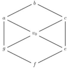
Example 2. Consider an instance (M, σ, p, 11, 2, 1) of the Offline TMP with
• the network G with a depot v0with arcs having uniform distance, see Figure 1,
a g b v0 f c e
Figure 1: This figure illustrates the network G of the instance (M, σ, p, 11, 2, 1) of the Offline TMP from Example 2.
• two unit-speed servers (i.e. two VIPAs that travel 1 unit of length in 1 unit of time) with
capacity Cap= 1 originally located at the depot v0,
• the following sequence σ of 6 requests:
r1= (0, a, c, 1, 4, 1) r3= (1, e, f, 2, 4, 1) r5 = (5, b, c, 6, 8, 1)
r2= (1, c, f, 6, 9, 1) r4= (3, b, a, 6, 9, 1) r6= (5, c, e, 5, 8, 1)
• profits p(rj)= 4d(xj, yj) for accepted requests rj.
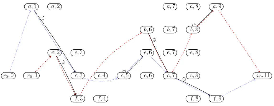
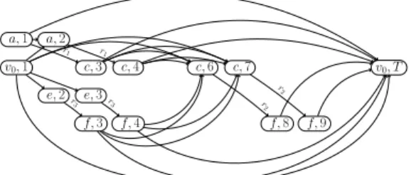
An optimal solution f∗ in the resulting time-expanded request network GT is illustrated in
Figure 2. We have σA = {r1, r2, r3, r4, r5, r6} and the following tours for the two VIPAs:
Γ1= (v 0, 0) → (a, 1) r1 −→ (c, 3) → (c, 5)−→ (e, 6) → (c, 7)r6 −→ ( f , 9) → (vr2 0, T ) Γ2= (v 0, 1) → (e, 2) r3 −→ ( f , 3) → (b, 6)−→ (c, 7) → (b, 8)r5 −→ (a, 9) → (vr4 0, T )
The total number of accepted requests is 6 with profit 4 · 8 served with a total tour length of 18,
hence the value of the optimal offline solution is 14.
v0, 0 v0, 1 v0, 11 a, 1 a, 2 a, 7 a, 8 a, 9 b, 6 b, 7 b, 8 c, 3 c, 4 c, 5 c, 6 c, 7 c, 8 e, 2 e, 3 e, 6 e, 7 e, 8 f, 3 f, 4 f, 8 f, 9 r1 r2 r 3 r4 r 5 r6
Figure 2: This figure shows the arcs with positive flow in the time-expanded request network GT for the instance
(M, σ, p, 11, 2, 1) of the Offline TMP from Example 2. The computed flow f∗in the time-expanded request network G T
can be interpreted as transportation schedule. The tour of the first VIPA is indicated by dashed arcs, and the tour of the second VIPA by dotted arcs. The total number of accepted requests is 6 served with a total tour length of 18.
3.2. Solving the Online Taxi Mode Problem
To handle the online situation (where the requests in σ are released over time during a time horizon [0, T ]), we consider three approaches: besides a simple heuristic, we apply the two well-known meta-strategies Replan and Ignore that solve the online version of the PDP by solving a
sequence of offline subproblems for certain time intervals [t0, T0] within [0, T ] on accordingly
modified request networks.
Earliest Pickup Heuristic. This simple heuristic incrementally constructs tours by always
choos-ing from the subsequence σ(t0) of currently waiting requests this request with smallest possible
start time and appending it to the tour with shortest distance from its current end to the requested origin, or rejecting the request if it is not reachable from all tours. LetΓibe a tour and (vi, ti) be
its current end. A request rj= (tj, xj, yj, pj, qj, zj) is reachable from (vi, ti) if
ti+ d(vi, xj) ≤ qj− d(xj, yj)
is a possible pickup time of rj.
Algorithm 1 (Earliest Pickup Heuristic (EPH)) Input: (M, σ, p, T, k, Cap)
Output:σAand toursΓ1, . . . , Γk
1: initialize σA= ∅, σ(t0)= {rj∈σ : tj= 0}, and Γi= (v0, 0) for 1 ≤ i ≤ k
2: WHILE σ(t0) , ∅ DO:
select rj∈σ(t0) with tjminimal
let d= ∞ and ` = 0
FOR i= 1 to k DO:
IF rjis reachable from current end (vi, ti) ofΓiTHEN
let di= d(vi, xj), IF di< d THEN d = di, `= i
IF d= ∞ THEN reject rjand remove it from σ(t0) (as rjis not reachable from anyΓi)
ELSE
accept rjand move it from σ(t0) to σA
update tourΓ`toΓ`= Γ`→ (xj, tj+ d) → (yj, tj+ d + d(xj, yj)
update σ(t0) by newly released requests
3: close all tours by returning to the depot 4: return σAandΓ1, . . . , Γk
Example 3. Consider the instance (M, σ, p, 11, 2, 1) of the TMP from Example 2. EPH proceeds
with this request sequence σ as follows. At the beginning, EPH initializes σA= ∅, the two tours
Γ1= Γ2= (v
0, 0) and, as r1= (0, a, c, 1, 4, 1) is released at time t0= 0, σ(t0)= {r1}.
EPH takes r1and computes d= 1 and l = 1, updates Γ1to
Γ1= (v
0, 0) → (a, 1) r1
−→ (c, 3)
and moves r1from σ(t0) to σA. At time t0= 1, r2 = (1, c, f, 6, 9, 1) and r3 = (1, e, f, 2, 4, 1) are
released and enter σ(t0). By p
2 = 6 > 2 = p3, EPH selects r3 and computes d = 1 and l = 2,
updatesΓ2to
Γ2= (v
0, 1) → (e, 2) r3
−→ ( f , 3)
and moves r3from σ(t0) to σA. Now, σ(t0)= {r2} causes EPH to select r2. EPH computes d= 0
and l= 1, updates Γ1to
Γ1= (v
0, 0) → (a, 1) r1
−→ (c, 3) → (c, 6)−→ ( f , 8)r2
and moves r2from σ(t0) to σA. At time t0 = 3, r4 = (3, b, a, 6, 9, 1) is released and enters σ(t0).
EPH takes r4and computes d= 3 and l = 2, updates Γ2to
Γ2= (v
0, 1) → (e, 2) r3
−→ ( f , 3) → (b, 6)−→ (a, 7)r4
and moves r4 from σ(t0) to σA. At time t0 = 5, r5 = (5, b, c, 6, 8, 1), r6 = (5, c, e, 5, 8, 1) are
released and enter σ(t0). By p
5= 6 > 5 = p6, EPH selects r6and rejects it as it is not reachable
from the ends of both tours. Then r5is left and also rejected as it is not reachable, too. Finally,
EPH closes both tours by returning to the depot and returns σA= {r1, r2, r3, r4} and the following
tours for the two VIPAs: Γ1= (v 0, 0) → (a, 1) r1 −→ (c, 3) → (c, 6)−→ ( f , 8) → (vr2 0, 10) Γ2= (v 0, 1) → (e, 2) r3 −→ ( f , 3) → (b, 6)−→ (a, 7) → (vr4 0, 8)
The total number of accepted requests is 4 with profit 4 · 6 served with a total tour length of 14,
hence EPH(σ)= 10.
Ignore. Recall that the overall idea of an Ignore strategy is to construct, starting at time t0= 0, for
the subsequence σ(t0) of currently waiting requests a (partial) optimal offline solution (which
in-cludes to determine which requests from σ(t0) can be accepted, and to compute optimal (partial)
tours to serve them) and to completely perform these tours before it checks for newly released
requests, updates σ(t0) and computes an optimal offline solution for the new subsequence σ(t0).
In our case with several servers, some partial tours for σ(t0) may be shorter than others such
that waiting until all partial tours are completed may let some servers idle. Hence, we propose
a variant of Ignore that updates σ(t0) whenever (at least) one server becomes idle (as it finished
serving its tour) and plans new partial tours for σ(t0) with the k0currently idle servers, i.e., on the subset S (t0, k0) ⊆ {Γ1, . . . , Γk} of finishes subtours. This is summarized in the algorithm IGNORE.
Algorithm 2 (IGNORE) Input: (M, σ, p, T, k, Cap) Output:σAand toursΓ1, . . . , Γk
1: initialize t0= 0, σA= ∅, σ(t0)= ∅, and Γi= (v0, 0) for 1 ≤ i ≤ k
2: WHILE t0< T DO:
let k0be the number of currently idle servers
IF k0> 0 THEN:
update t0and σ(t0)= {rj∈σ : tj≤ t0}
call I-OFFLINE with σA, σ(t0) and the tours S (t0, k0) of the idle servers
completely perform the (modified) tours in S (t0, k0) 3: close all tours by returning to the depot
4: return σAandΓ1, . . . , Γk
To compute the optimal solutions for the subsequences σ(t0) with the help of I-OFFLINE, we
build a time-expanded request network GI(t0) in a similar way as GTfor the offline situation. The
only difference is that we do not have a single source (as (v0, 0) in GT), but that we need to use
the current positions of the idle VIPAs as sources (i.e., the current ends of the tours in S (t0, k0)),
collected in a position vector P(t0) with t0as start time. Accordingly, we obtain
V+= {(Pi(t0), t0) : (Pi(t0), t0) current end of tourΓi∈ S (t0, k0)}
as set of source nodes and add the arcs from (Pi(t0), t0) to the sink (v0, T ) for all such nodes. In
GI(t0), we solve the max profit flow problem (1) where (1b) is replaced by
X
a∈δ+(v,t0)
f(a)= k0(v) ∀(v, t0) ∈ V+ 10
and k0(v) denotes the number of idle VIPAs situated in v at time t0(thus all k0(v) sum up to k0).
From the flow computed in GI(t0), it is straitforward to determine newly accepted requests
(corresponding to request arcs a ∈ ARwith f (a) > 0) and to construct (partial) toursΓ1, . . . , Γk
for the VIPAs in the same way as described for the offline situation (thereby ignoring sink arcs).
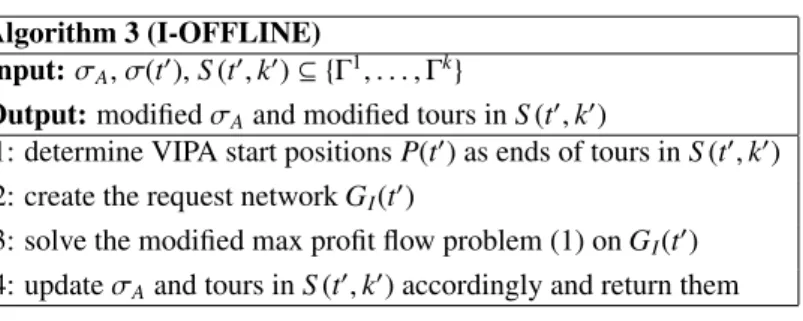
The whole process can be summarized in the algorithm I-OFFLINE. Algorithm 3 (I-OFFLINE)
Input:σA, σ(t0), S (t0, k0) ⊆ {Γ1, . . . , Γk}
Output: modified σAand modified tours in S (t0, k0)
1: determine VIPA start positions P(t0) as ends of tours in S (t0, k0) 2: create the request network GI(t0)
3: solve the modified max profit flow problem (1) on GI(t0)
4: update σAand tours in S (t0, k0) accordingly and return them
Example 4. Consider the instance (M, σ, p, 11, 2, 1) of the TMP from Example 2. IGNORE
proceeds with this request sequence σ as follows. At the beginning, IGNORE initializes σA = ∅,
σ(t0)= ∅, and the two tours Γ1= Γ2= (v
0, 0). At time t0= 0, both VIPAs are idle s.t. k0= 2 > 0.
Request r1 = (0, a, c, 1, 4, 1) is released and moves from σ to σ(t0). IGNORE computes the
partial offline solution for σ(t0)= {r
1} and P(t0) = (v0, v0) on the network GI(0), see Figure 3.
IGNORE solves the max profit flow problem (1) on GI(0), obtains
v0, 0 v0, T
a, 1 a, 2
c, 3 c, 4
r1 r1
Figure 3: The request network GI(0) for Ignore.
Γ1= (v 0, 0) → (a, 1) r1 −→ (c, 3) Γ2= (v 0, 0)
moves r1from σ(t0) to σAand starts VIPA 1 to serveΓ1, whereas VIPA 2 stays idle in the depot.
At time t0= 1, r2 = (1, c, f, 6, 9, 1) and r3 = (1, e, f, 2, 4, 1) are released and move from σ to
σ(t0). As VIPA 2 is idle, IGNORE computes the partial offline solution for σ(t0)= {r
2, r3} and
P(t0)= (−, v0) on the network GI(1), see Figure 4. IGNORE solves the modified max profit flow
problem (1) on GI(1), obtains Γ2 = (v 0, 1) → (e, 2) r3 −→ ( f , 3) → (c, 6)−→ ( f , 8)r2 11
v0, 1 c, 6 c, 7 v0, T e, 2 e, 3 f, 3 f, 4 f, 8 f, 9 r3 r3 r2 r2
Figure 4: The request network GI(1) for Ignore.
moves r2, r3from σ(t0) to σAand starts VIPA 2 to serveΓ2.
At time t0 = 3, Γ1is served by VIPA 1, r4 = (3, b, g, 6, 9, 1) is released and moves from σ
to σ(t0). IGNORE computes the partial offline solution for σ(t0)= {r4} and P(t0)= (c, −) on the
network GI(3), see Figure 5. IGNORE solves the modified max profit flow problem (1) on GI(3),
v0, T c, 3 b, 6 b, 7 b, 8 a, 7 a, 8 a, 9 r 4 r4 r4
Figure 5: The request network GI(3) for Ignore.
obtains
Γ1= (c, 3) → (b, 6) r4
−→ (a, 7)
moves r4from σ(t0) to σAand starts VIPA 1 to serveΓ1.
At time t0 = 7, Γ1 is served by VIPA 1, hence IGNORE checks for newly released requests
and updates σ(t0) = {r5, r6}. IGNORE computes the partial offline solution for σ(t0)= {r5, r6}
and P(t0)= (a, −) on the network GI(7), see Figure 6. and obtains that none of r5, r6is reachable
v0, T c, 5 c, 6 c, 7 c, 8 b, 6 b, 7 a, 7 e, 6 e, 7 e, 8 r5 r5 r6 r6 r6
Figure 6: The request network GI(7) for Ignore.
from (a, 7) such that both r5, r6are rejected. Finally, IGNORE closes both tours by returning to
the depot and returns σA = {r1, r2, r3, r4} and the following tours for the two VIPAs:
Γ1= (v 0, 0) → (a, 1) r1 −→ (c, 3) → (b, 6)−→ (a, 7) → (vr4 0, 8) Γ2= (v 0, 2) → (e, 3) r3 −→ ( f , 4) → (c, 6)−→ ( f , 8) → (vr2 0, 10)
The total number of accepted requests is 4 with profit 4 · 6 served with a total tour length of 14,
hence IGNORE(σ)= 10.
Replan. Recall that the overall idea of a replan strategy is to consider at each moment in time
t0∈ [0, T ] the subsequence σ(t0) of currently waiting requests, to determine which requests from
σ(t0) can be accepted, to compute optimal (partial) tours to serve them, and to perform these tours
until new requests are released and to recompute σ(t0) and the tours (keeping already accepted
requests).
Hereby, finding optimal (partial) tours corresponds to solve, in each replanning step, an
opti-mal offline solution on the subsequence σ(t0). This is summarized in the algorithm REPLAN.
Algorithm 4 (REPLAN) Input: (M, σ, p, T, k, Cap) Output:σAand toursΓ1, . . . , Γk
1: initialize σA= ∅, σ(t0)= {rj∈σ : tj= 0}, and Γi= (v0, 0) for 1 ≤ i ≤ k
2: WHILE t0< T DO: call R-OFFLINE(σA, σ(t0),Γ1, . . . , Γk)
perform the (modified) tours until new requests become known, update t0and σ(t0)
3: return σAandΓ1, . . . , Γk
To compute those optimal solutions for the subsequences σ(t0), we build a time-expanded
request network GR(t0)= (V0, A0) based on σ(t0) and the original network G and consider a flow
in GR(t0) that corresponds to the studied (partial) tours.
We construct GR(t0) = (V0, A0) in a similar way as GT for the offline situation. The main
difference is that we do not have a single source (as (v0, 0) in GT), but that we need to use the
possible start positions and possible start times of the VIPAs as sources.
For that, we extract the possible start positions P(t0) and start times S (t0) for the VIPAs from the current toursΓ1, . . . , Γk. At the beginning, i.e. at time t= 0, we clearly have P(t0)
i= v0and
S(t0)i= 0. At any later time point t0, the start positions and start times are as follows: if VIPA i
is currently serving a request rj, then we have P(t0)i = yjand S (t0)i = t drop
j ; otherwise, P(t
0) iis
the current position v of VIPA i and S (t0)i= t0.
Accordingly, the node set V0= V+∪ Vx∪ Vy∪ (v0, T0) is composed of
• the VIPAs start positions and start times (P(t0)
i, S (t0)i) for 1 ≤ i ≤ k as sources in V+,
• all possible origins (xj, tpickj ) of all rj∈σ(t0) and all pj≤ tpickj ≤ qj− d(xj, yj) in Vx,
• all possible destinations (yj, t drop
j ) of all rj∈σ(t0) and all pj+ d(xj, yj) ≤ t drop
j ≤ qjin Vy,
• a sink node (v0, T0) with T0= max{tdropj , rj∈σ(t0)}.
The arc set A0= A+∪ AR∪ AL∪ A−is composed of
• source arcs from all nodes (P(t0)i, S (t0)i) ∈ V+to all reachable origins (xj, t pick
j ) ∈ Vxwith
t0+ d(v, xj) ≤ t pick j ,
• request arcs from each (xj, t
pick
j ) ∈ Vxto (yj, t pick
j + d(xj, yj)) ∈ Vyin AR,
• link arcs from all destinations (yj, tdropj ) ∈ Vyto all reachable origins (xi, tipick) ∈ Vxwith
tdropj + d(yj, xi) ≤ tipickin AL,
• sink arcs from all destinations (yj, t drop
j ) ∈ Vyto (v0, T0) in A−.
To keep previously accepted requests, we partition σ(t0) into the subsequences
• σA(t0) of previously accepted but until time t0not yet served requests and
• σN(t0)= {rj∈σ : tj= t0} of requests that are newly released at time t0,
and partition the request arcs accordingly in ARA and ARN. Moreover, we distinguish the subsets
ARj
Aand A
j
RN of request arcs of the corresponding previously accepted request rj ∈ σA(t
0) resp.
newly released request rj∈σN(t0).
In GR(t0), we solve the following max profit flow problem
max X
a∈AR
p(a) f (a) −X
a∈A0
c(a) f (a) (2a)
s.t. X a∈δ+(v,t) f(a)= k(v) ∀(v, t) ∈ V+ (2b) X a∈δ−(v,t) f(a)= X a∈δ+(v,t) f(a) ∀(v, t) ∈ Vx∪ Vy (2c) X a∈Aj RA f(a)= 1 ∀ARAj ⊆ ARA (2d) X a∈ARNj
f(a) ≤ 1 ∀ARNj ⊆ ARN (2e)
f(a) ≥ 0 ∀a ∈ A0 (2f)
f(a) ∈ Z ∀a ∈ A0 (2g)
where again δ−(v, t) denotes the set of outgoing arcs of (v, t), δ+(v, t) the set of incoming arcs of
(v, t) and k(v) the number of VIPAs initially situated in v.
Constraints (2d) ensure that previously accepted requests are served whereas constraints (2e) allow to reject newly released requests.
Source, flow conservation and nonnegativity constraints (2b), (2c), (2f) together give again rise to a totally unimodular matrix, but due to (2d) and (2e) the entire constraint matrix is not totally unimodular s.t. integrality constraints (2g) are again required.
From the computed flow f0 in the request network GR(t0), it is straitforward to determine
newly accepted requests (corresponding to request arcs a ∈ ARN with f0(a) > 0) and to construct
(partial) toursΓ1, . . . , Γkfor the VIPAs in the same way as described for the offline situation.
The whole process can be summarized in the algorithm R-OFFLINE. Algorithm 2 (R-OFFLINE)
Input:σA, σ(t0),Γ1, . . . , Γk
Output: modified σAand modified toursΓ1, . . . , Γk
1: determine VIPA start positions P(t0) and start times S (t0) fromΓ1, . . . , Γk
2: create the request network GR(t0)
3: solve the max profit flow problem (2) on GR(t0)
4: update σAandΓ1, . . . , Γkaccordingly and return them
Example 5. Consider the instance (M, σ, p, 11, 2, 1) of the TMP from Example 2. REPLAN
proceeds with this request sequence σ as follows. At the beginning, REPLAN initializes σA = ∅,
and the two toursΓ1 = Γ2 = (v
0, 0). At time t0= 0, r1 = (0, a, c, 1, 4, 1) is released. REPLAN
computes the partial offline solution for σA(0)= ∅, σN(0)= {r1}, S (0)= (0, 0) and P(0) = (v0, v0)
on the network GR(0), see Figure 7. REPLAN solves the max profit flow problem (2) on GR(0),
v0, 0 v0, T
a, 1 a, 2
c, 3 c, 4
r1 r1
Figure 7: The request network GR(0) from Example 5.
obtains Γ1 = (v 0, 0) → (a, 1) r1 −→ (c, 3) → (v0, T ) Γ2 = (v 0, 0) → (v0, T )
accepts r1and moves VIPA 1 towards a.
At time t0= 1, r
2= (1, c, f, 6, 9, 1) and r3= (1, e, f, 2, 4, 1) are released. REPLAN computes the
partial optimal offline solution for σA(1)= {r1}, σN(1)= {r2, r3}, S (1)= (1, 1) and P(1) = (a, v0)
on the network GR(1), see Figure 8.
v0, 1 v0, T a, 1 a, 2 c, 3 c, 4 c, 6 c, 7 e, 2 e, 3 f, 3 f, 4 f, 8 f, 9 r1 r1 r2 r2 r3 r3
Figure 8: The request network GR(1) from Example 5.
REPLAN solves the max profit flow problem (2) on GR(1), obtains
Γ1= (a, 1)−→ (c, 3) → (c, 6)r1 −→ ( f , 8) → (vr2 0, T ) Γ2= (v 0, 1) → (e, 2) r3 −→ ( f , 3) → (v0, T )
accepts r2and r3, moves VIPA 1 towards c (serving r1) and VIPA 2 towards e.
At time t0= 3, r1and r3are served and r4 = (3, b, a, 6, 9, 1) is released. REPLAN computes the
partial optimal offline solution for σA(3)= {r2}, σN(3)= {r4}, S (3)= (3, 3) and P(3) = (c, f ) on
the network GR(3), see Figure 9.
REPLAN solves the max profit flow problem (2) on GR(3), obtains
Γ1 = (c, 3) → (c, 6)−r2→ ( f , 8) → (v 0, T )
Γ2 = ( f, 3) → (b, 6)−r4→ (a, 7) → (v 0, T )
v0, T c, 3 c, 6 c, 7 f, 3 f, 8 f, 9 b, 6 b, 7 b, 8 a, 7 a, 8 a, 9 r2 r2 r4 r4 r4
Figure 9: The request network GR(3) from Example 5.
and accepts r4. REPLAN moves VIPA 2 towards (b, 6) on one of the two shortest paths s.t.
VIPA 2 moves either towards e and then towards c or towards g and then towards a. In both cases VIPA 2 can reach (b, 6).
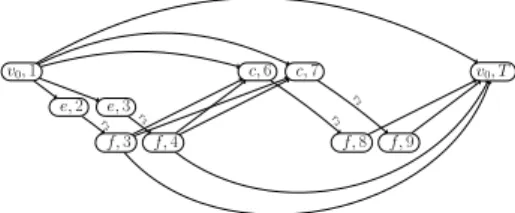
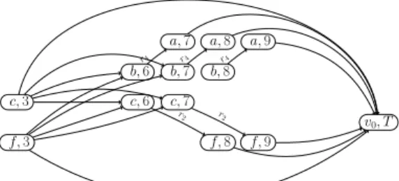
At time t0 = 5, r5 = (5, b, c, 6, 8, 1), r6 = (5, c, e, 5, 8, 1) are released. REPLAN computes
the partial optimal offline solution for σA(5) = {r2, r4}, σN(5) = {r5, r6}, S (5) = (5, 5) and
P(5) = (c, c) on the network GR(5), see Figure 10. Note that the tours obtained do not change
whether P(5)= (c, a) or P(5) = (c, c). In Figure 10, P(5) = (c, c). v0, T c, 5 c, 6 c, 7 c, 8 f, 8 f, 9 b, 5 b, 6 b, 7 b, 8 a, 7 a, 8 a, 9 e, 6 e, 7 e, 8 r2 r2 r4 r4 r4 r5 r5 r5 r 6 r6 r6
Figure 10: The request network GR(5) from Example 5.
REPLAN solves the max profit flow problem (2) on GR(5), obtains
Γ1 = (c, 5) r6
−→ (e, 6) → (c, 7)−→ ( f , 9) → (vr2 0, T )
Γ2 = (c, 5) → (b, 6) r5
−→ (c, 7) → (b, 8)−r→ (a, 9) → (v4 0, T )
and accepts r5and r6.
In total, REPLAN accepts all 6 requests with σA = {r1, r2, r3, r4, r5, r6} and serves them by the
tours Γ1= (v 0, 0) → (a, 1) r1 −→ (c, 3) → (c, 5)−→ (e, 6) → (c, 7)r6 −→ ( f , 9) → (vr2 0, T ) Γ2= (v 0, 0) → (v0, 1) → (e, 2) r3 −→ ( f , 3) → (b, 6)−r5→ (c, 7) → (b, 8)−→ (a, 9) → (vr4 0, T )
with a total tour length of 18, and a profit 4 · 8 hence REPLAN(σ)= 14.
Discussion of the approaches. In view of the behavior of the three proposed algorithms
ob-served on the instance from Example 2, we note that requests that are released long time
be-fore the time window to serve them cause difficulties for all three algorithms. Such a request
rj= (tj, xj, yj, pj, qj, zj) (like r2in the example) causes
• EPH and IGNORE to construct a tourΓiserving r
jat its end where VIPA i stays idle within
Γiuntil p
j(seeΓ1of EPH between (c, 3) and (c, 6)= (x2, p2) when VIPA 1 starts to serve
r2) whereas other requests released meanwhile are not reachable from the end ofΓi(like
r5, r6in the example).
• REPLAN to accept rj which may cause later to reject other requests released later on if
they cannot be integrated into a tour serving rj.
Moreover, while EPH and REPLAN check newly released requests immediately and also decide
immediately about their acceptance/ rejection, IGNORE checks for newly released requests only
when a VIPA becomes idle. This may result in late decisions about the acceptance/ rejection
of requests (like for r5, r6in the example which are rejected shortly before the end of their time
window, at the latest possible pickup time), and may even result in a rejection after the time window of the request.
Hence, we conclude that (even the here considered variant of) IGNORE is not suitable for the Online TMP since the way how to construct tours may result in many rejected requests and
the decision to accept/reject a request may be taken late, which does not comply to the
quality-of-service aspect of the fleet management. Therefore, we focus on the other two approaches and perform computational results only for EPH and REPLAN, with the expectation that EPH is faster, but REPLAN achieves a higher acceptance rate.
4. Evaluating the performance of the online strategies
We shall evaluate the online algorithms EPH and REPLAN in a two-fold manner: • in theory with the help of competitive analysis (Section 4.1),
• in practice with the help of some computational results (Section 4.2). 4.1. Competitive analysis
It is standard to evaluate the quality of online algorithms with the help of competitive analysis. A detailed introduction to online optimization and competitive analysis can be found e.g. in the book by Borodin and El-Yaniv [8].
Competitive analysis can be viewed as a game between an online algorithm ALG and a malicious adversary who tries to generate a worst-case request sequence σ which maximizes the ratio between the online cost ALG(σ) and the optimal cost OPT(σ) where the adversary knows the entire request sequence σ in advance.
An online algorithm ALG for an online maximization problem is called c-competitive if ALG produces for any request sequence σ of the studied problem a feasible solution with costs ALG(σ) such that
OPT(σ) ≤ c · ALG(σ)
for some given c ≥ 1. The competitive ratio of ALG is the infimum over all c such that ALG is c-competitive.
We are interested in analyzing the online algorithms EPH and REPLAN for the Online TMP. In fact, we obtain the more general result that no (deterministic) online algorithm ALG for the Online TMP is competitive against a common type of adversary.
An oblivious adversary knows the complete behavior of a (deterministic) online algorithm ALG and chooses a worst-case sequence for ALG. Hereby, an oblivious adversary is allowed to
move VIPAs towards the origins xjof not yet released requests rj (but also has to respect the
time windows [pj, qj] to serve accepted requests rj).
We show that an oblivious adversary can force any (deterministic) online algorithm ALG for the Online TMP to reject all requests of a sequence while the adversary can accept and serve all requests, implying that ALG is not competitive.
Theorem 6. There is no competitive (deterministic) online algorithm for the Online TMP against an oblivious adversary.
Proof. The idea for a worst case sequence for an online algorithm ALG is as follows. The
adversary releases the requests rj ∈ σ in such a way that the delay between the release date tj
and the latest possible pickup time qj− d(xj, yj) is smaller than the distance d(v0, xj). That way,
ALG has to reject all requests (and its VIPA stays in the depot v0), whereas the adversary moves
its VIPA already towards the origin x0 of the first request r0 before r0 has been released and is
able to arrive at x0at time q0− d(x0, y0) and can accept and serve r0and all following requests in
the sequence σ. For that, we consider an instance (M, σ, p, T, 1, 1) of the Online TMP with
• the network G with depot v0from Figure 11
v0 v2 v1 2 2 1
Figure 11: This figure illustrates the network G of the instance (M, σ, p, T, 1, 1) of the Online TMP with an oblivious adversary.
• the following sequence σ= {r0, r1, r2, . . . , r`} of requests with
rj= ( j + 1, v1, v2, j + 2, j + 3, 1) for all even j with 0 ≤ j ≤ `,
rj= ( j + 1, v2, v1, j + 2, j + 3, 1) for all odd j with1 ≤ j ≤ `,
• profits p(rj)= 2d(xj, yj) for accepted requests rj.
The online algorithm ALG treats the sequence σ as follows. At time t = 1, the first request
r0 = (1, v1, v2, 2, 3, 1) is released. As the origin x0 = v1 of r0 is not reachable from the depot
before or at the latest possible pickup time q0− d(v1, v2)= 2 due to d(v0, v1)= 2, ALG rejects r0
and the VIPA operated by ALG stays in the depot v0. At time t= 2, request r1 = (2, v2, v1, 3, 4, 1)
is released. Again, the origin x1 = v2of r1is not reachable from the depot before or at the latest
possible pickup time q1− d(v1, v2)= 3 due to d(v0, v2)= 2. Hence, ALG also rejects r1and the
VIPA operated by ALG stays in v0. This is repeated for any further request rl ∈ σ so that all
rj∈σ are rejected by ALG and we clearly have
ALG(σ)= 0.
In contrary, the adversary moves its VIPA at time t= 0 from the depot v0towards x0= v1, arrives
at p0 = 2 in v1 and accepts and serves r0by moving to y0 = v2, arriving there at time 3 = p1,
Thus, the adversary can accept and serve r1by moving to v1= y1, arriving there at time 4= p2.
This is repeated for any further request rjin σ (that the VIPA operated by the adversary always
arrives at xjat time pj) so that the adversary can accept and serve all requests rjin σ. At the end
of the sequence the adversary returns its VIPA to the depot to close its tour. Thus we obtain OPT(σ)= (` + 1) · 2d(v1, v2) − ((`+ 1) · d(v1, v2)+ 2 + 2) = (` + 1) · d(v1, v2) − 4= ` − 3.
This shows
OPT(σ)
ALG(σ) = ∞
so that there is no finite number c bounding the ratio between OPT(σ) and ALG(σ) for all possible request sequences σ of the Online TMP.
Since the worst-case request sequence used to show the non-competitivity result is only based on the reachability of requests, but not on a particular strategy of an online algorithm, we con-clude:
Corollary 7. Neither EPH nor REPLAN is competitive for the Online TMP against an oblivious adversary.
4.2. Computational results
This section deals with computational experiments for the optimal offline solution of the
TMP, the heuristic EPH and the replan strategy for the Online TMP. In fact, due to the very special request structures of the previously presented worst-case instances to prove the non-competitiveness of any online algorithm for the Online TMP, we expect a better behavior of the proposed strategies for the Online TMP in average.
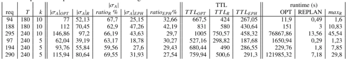
The computational results presented in Table 1 support this expectation. They compare the total number of accepted (and thus served) requests by EPH and REPLAN with the optimal
offline solution OPT. The computations use randomly generated instances with 20 stations, 5
to 10 VIPAs, time-horizons between 180 and 240 time units, and between 90 and 300 cus-tomer requests. These instances are based on the network from the industrial site of Michelin at Clermont-Ferrand and randomly generated request sequences resembling typical instances that occurred during an experimentation in Clermont-Ferrand performed from October 2015 until February 2016 [24].
The operating system for all tests is Linux CentOS with kernel version 2.6.32 clocked at 2.40 GHz, with 1 TB RAM. The approaches are implemented in Python and Gurobi 8.21 is used for solving the ILPs. The results are summarized in Table 1.
EPH computes in very short times solutions (always less than 1 second), but can only reach
in average an acceptance rate of about 32% compared to the optimal offline solution OPT.
Also REPLAN computes solutions for each replanning step within a short time, and can
achieve a reasonable ratio w.r.t. the total number of accepted requests between the optimal offline
solution OPT and REPLAN (in average around 65%).
5. Concluding remarks
We note for the Offline TMP, that in the special case of tight time windows satisfying pj+
d(xj, yj)= qj(which clearly results in pj = tpickj and qj = tdropj ) for all rj ∈σ, there is exactly
one request arc per request s.t. the constraints (1d) reduce to
f(a) ≤ 1 for all a ∈ AR. (3)
Table 1: This table shows the computational results for 600 test instances of EPH and REPLAN in comparison to OFFLINE for the TMP. The instances are grouped by the number of requests (1st column), the time horizon (2nd column) and the number of VIPAs (3rd column) with 100 instances per parameter set. Average values are shown for the total number |σA| of accepted requests of OFFLINE, REPLAN and EPH and the ratio between them (REPLANOPT and
EPH OPT)
and for the total tour length T T L needed to serve the accepted requests. Finally we provide the time needed to compute the optimal offline solution, the average runtime of REPLAN per recomputation step and the maximum runtime maxRof
the recomputation steps of REPLAN. The average runtime of EPH is not shown as it never exceeds one second.
|σA| TTL runtime (s)
req T k |σA|OPT |σA|R ratioR% |σA|EPH ratioEPH% T T LOPT T T LR T T LEPH OPT REPLAN maxR 94 180 10 77 52,13 67,7 25,15 32,66 667,5 424 267,05 11,9 0,49 1,6 188 180 10 112 70,45 62,9 47,26 42,19 831 580 430,64 151 3 10,83 295 240 10 146,86 97,2 66,19 43,63 29,7 1005 750,57 458,32 76867,86 13,56 45,54 97 240 5 62,04 39,19 63,17 18,78 30,27 527,16 298,82 187,68 1650,94 0,29 1,23 194 240 5 93,76 55,84 59,56 27,6 29,43 680,44 490 286,55 229,76 1,8 7,85 290 240 5 115,94 80,64 69,55 31,93 27,54 759,94 500,6 291,3 121985,32 7,18 29,8
Therefore, in the case with tight time windows, the totally unimodular matrix implied by the source and flow conservation constraints (i.e., the node-arc incidence matrix of the digraph
un-derlying GT) is only composed with identity matrices (for the nonnegativity and the capacity
constraints (3)) such that the entire constraint matrix becomes totally unimodular. This implies:
Corollary 8. The Offline Taxi Mode Problem with tight time windows can be solved in
polyno-mial time.
In the general case, this is not true, but our experiments showed that the running times to
solve the Offline Taxi Mode Problem are still reasonable, see Table 1.
Regarding the quality of the solutions obtained by EPH and REPLAN, we summarize from the previous section that
• in theory, neither EPH nor REPLAN is competitive against an oblivious adversary since for all (deterministic) online algorithms ALG for the Online TMP, there is no finite c s.t. for all instances σ we have that ALG(σ) ≥ c OPT(σ);
• in practice, EPH is faster, REPLAN provides solutions of reasonably quality within short time for each recomputation step and achieves a better acceptance rate, see again Table 1. We can conclude that the here proposed REPLAN strategy is already a promising algorithm to handle the Online TMP for the taxi mode in the studied VIPAFLEET management system.
As future work, we plan to improve the runtime of REPLAN by reducing the time-expanded network built in each replanning step without loss of optimality. Such an approach has been applied by [7] to a service network design problem and by [21] to a multi-depot multi-vehicle bus scheduling problem for timetabled trips (by using time-space-based instead of connection-based networks which leads to a crucial reduction of the size of the mathematical models).
We also plan to study another variant of the TMP without the here required condition that, at
each time, at most one request rjcan be served by a VIPA and that this has to be done in a direct
way along a shortest path from xjto yj. Dropping this condition would open the possibility to
serve several requests simultaneously by a same VIPA (as long as the capacity Cap is respected),
but that while serving request rj, sometimes detours are necessary to stations not lying on a
short-est path from xjto yj in order to pickup or drop passengers from other requests. This problem
variant will lead to a more complex model and also computing solutions is more involved, but may lead to a higher rate of accepted requests and, therefore, to a higher quality-of-service level for the fleet management.
References
[1] Ravindra K Ahuja, Thomas L Magnanti, and James B Orlin. Network flows: theory, algorithms, and applications. 1993.
[2] Norbert Ascheuer, Sven O Krumke, and J¨org Rambau. The online transportation problem: competitive scheduling of elevators. ZIB, 1998.
[3] Norbert Ascheuer, Sven O Krumke, and J¨org Rambau. Online dial-a-ride problems: Minimizing the completion time. In STACS 2000, pages 639–650. Springer, 2000.
[4] Giorgio Ausiello, Esteban Feuerstein, Stefano Leonardi, Leen Stougie, and Maurizio Talamo. Competitive al-gorithms for the on-line traveling salesman. In Workshop on Alal-gorithms and Data Structures, pages 206–217. Springer, 1995.
[5] Giorgio Ausiello, Esteban Feuerstein, Stefano Leonardi, Leen Stougie, and Maurizio Talamo. Algorithms for the on-line travelling salesman 1. Algorithmica, 29(4):560–581, 2001.
[6] Gerardo Berbeglia, Jean-Franc¸ois Cordeau, and Gilbert Laporte. Dynamic pickup and delivery problems. European journal of operational research, 202(1):8–15, 2010.
[7] Natashia Boland, Mike Hewitt, Luke Marshall, and Martin Savelsbergh. The continuous-time service network design problem. Operations Research, 2017.
[8] Allan Borodin and Ran El-Yaniv. Online computation and competitive analysis. cambridge university press, 2005. [9] Sahar Bsaybes. Mod`eles et algorithmes de gestion de flottes de v´ehicules VIPA. PhD thesis, Universit´e Clermont
Auvergne, 2017.
[10] Sahar Bsaybes, Alain Quilliot, and Annegret K Wagler. Fleet management for autonomous vehicles. arXiv preprint arXiv:1703.10565, 2017.
[11] Sahar Bsaybes, Alain Quilliot, and Annegret K Wagler. Fleet management for autonomous vehicles using flows in time-expanded networks. Electronic Notes in Discrete Mathematics (special issue of LAGOS 2017), 62:255–260, 2017.
[12] Jean-Franc¸ois Cordeau and Gilbert Laporte. The dial-a-ride problem: models and algorithms. Annals of Operations Research, 153(1):29–46, 2007.
[13] Samuel Deleplanque and Alain Quilliot. Transfers in the on-demand transportation: the DARPT Dial-a-Ride Prob-lem with transfers allowed. In Multidisciplinary International Scheduling Conference: Theory and Applications (MISTA), number 2013, pages 185–205, 2013.
[14] Anke Fabri and Peter Recht. Online dial-a-ride problem with time windows: an exact algorithm using status vectors. In Operations Research Proceedings 2006, pages 445–450. Springer, 2007.
[15] Lester R Ford Jr and Delbert Ray Fulkerson. Constructing maximal dynamic flows from static flows. Operations research, 6(3):419–433, 1958.
[16] Martin Groß and Martin Skutella. Generalized maximum flows over time. In International Workshop on Approxi-mation and Online Algorithms, pages 247–260. Springer, 2011.
[17] Martin Gr¨otschel, Sven O Krumke, J¨org Rambau, Thomas Winter, and Uwe T Zimmermann. Combinatorial online optimization in real time. In Online optimization of large scale systems, pages 679–704. Springer, 2001. [18] http://www.easymile.com. Easymile, 2015.
[19] http://www.ligier.fr. Ligier group, 2015. [20] http://www.viameca.fr. Viam´eca, 2015.
[21] Natalia Kliewer, Taieb Mellouli, and Leena Suhl. A time–space network based exact optimization model for multi-depot bus scheduling. European journal of operational research, 175(3):1616–1627, 2006.
[22] Ronald Koch, Ebrahim Nasrabadi, and Martin Skutella. Continuous and discrete flows over time. Mathematical Methods of Operations Research, 73(3):301, 2011.
[23] Jan Karel Lenstra and AHG Kan. Complexity of vehicle routing and scheduling problems. Networks, 11(2):221– 227, 1981.
[24] E Royer, F Marmoiton, S Alizon, D Ramadasan, M Slade, A Nizard, M Dhome, B Thuilot, and F Bonjean. Retour dexp´erience apr`es plus de 1000 km en navette sans conducteur guid´ee par vision.
[25] Eric Royer, Jonathan Bom, Michel Dhome, Benoit Thuilot, Maxime Lhuillier, and Franc¸ois Marmoiton. Out-door autonomous navigation using monocular vision. In Intelligent Robots and Systems, 2005.(IROS 2005). 2005 IEEE/RSJ International Conference on, pages 1253–1258. IEEE, 2005.
[26] Jian Yang, Patrick Jaillet, and Hani Mahmassani. Real-time multivehicle truckload pickup and delivery problems. Transportation Science, 38(2):135–148, 2004.