Origin of ferromagnetism and magnetic anisotropy in a family of copper(II) triangles

HAL Id: hal-02866491

https://hal.archives-ouvertes.fr/hal-02866491

HAL is a multi-disciplinary open access archive for the deposit and dissemination of sci-entific research documents, whether they are pub-lished or not. The documents may come from teaching and research institutions in France or abroad, or from public or private research centers.

L’archive ouverte pluridisciplinaire HAL, est destinée au dépôt et à la diffusion de documents scientifiques de niveau recherche, publiés ou non, émanant des établissements d’enseignement et de recherche français ou étrangers, des laboratoires publics ou privés.

Origin of ferromagnetism and magnetic anisotropy in a

family of copper(II) triangles

Logesh Mathivatanan, Guillaume Rogez, Nadia Ben Amor, Vincent Robert,

Raphael Raptis, Athanassios Boudalis

To cite this version:

Logesh Mathivatanan, Guillaume Rogez, Nadia Ben Amor, Vincent Robert, Raphael Raptis, et al.. Origin of ferromagnetism and magnetic anisotropy in a family of copper(II) triangles. Chemistry -A European Journal, Wiley-VCH Verlag, 2020, 26 (56), pp.12769-12784. �10.1002/chem.202001028�. �hal-02866491�

1

Origin of ferromagnetism and magnetic anisotropy in a family of

copper(II) triangles

Logesh Mathivatanan,1 Guillaume Rogez,2 Nadia Ben Amor,3 Vincent Robert,4 Raphael G. Raptis,1

Athanassios K. Boudalis*4

1

Department of Chemistry and Biochemistry and the Biomolecular Sciences Institute, Florida International University, Miami, FL 33199, USA.

2

Université de Strasbourg, CNRS, Institut de Physique et Chimie des Matériaux de Strasbourg (IPCMS), UMR 7504, F-67000 Strasbourg, France.

3

Laboratoire de Chimie et Physique Quantiques UMR 5626, CNRS/Université Paul Sabatier - Bat. 3R1B4, 118 route de Narbonne 31062 Toulouse Cedex 09, France

4

Institut de Chimie de Strasbourg (UMR 7177, CNRS-Unistra), Université de Strasbourg, 4 rue Blaise Pascal, CS 90032, F-67081 Strasbourg, France. E-mail: bountalis@unistra.fr.

Abstract

Previously reported ferromagnetic triangles (NnBu4)2[Cu3(μ3-Cl)2(μ-4-NO2-pz)3Cl3] (1),

(PPN)2[Cu3(μ3-Cl)2(μ-pz)3Cl3] (2), (bmim)2[Cu3(μ3-Cl)2(μ-pz)3Cl3] (3) and newly reported

(PPh4)2[Cu3(μ3-Cl)2(μ-4-Ph-pz)3Cl3] (4) were studied by magnetic susceptometry, Electron

Paramagnetic Resonance (EPR) spectroscopy and ab initio calculations to assess the origins of their

ferromagnetism and of the magnetic anisotropy of their ground S = 3/2 state (PPN+ =

bis(triphenylphosphine)iminium, bmim+ = 1-butyl-3-methylbenzimidazolium). Ab initio studies

revealed the d_z2 character of the magnetic orbitals of the compressed trigonal bipyramidal copper(II)

ions. Ferromagnetic interactions were attributed to weak orbital overlap via the pyrazolate bridges. From the wavefunctions expansions, the ratios of the magnetic couplings was determined, which was indeterminate by magnetic susceptometry. Single-crystal EPR studies of 1 were carried out to extend the spin Hamiltonian with terms which induce zero-field splitting (zfs), namely dipolar interactions, anisotropic exchange and Dzyaloshinskii-Moriya interactions (DMI). The data were treated through both a giant-spin model and through a multispin exchange-coupled model. The latter indicated that ~62% of the zfs is due to anisotropic and ~38% due to dipolar interactions. The powder EPR data of all complexes were fitted to a simplified form of the multispin model and the anisotropic and dipolar contributions to the ground state zfs were estimated.

2

Introduction

Triangular Molecular NanoMagnets (MNMs) comprising half-integer spins (e.g., CuII, S = 1/2; FeIII,

S = 5/2) present particularly diverse interest. Historically, they were the first complexes for which the

multispin Hamiltonian approach was properly implemented, in Kambe’s seminal work.1 Over time,

their relevance has extended to various domains, ranging from biology to spintronics. E.g. their molecular and magnetic structures make them ideal models for the trimetallic active sites of various

bioinorganic systems like the [3Fe-3S] centers in ferredoxins,2,3 or the active sites of particulate

Methane Monoxygenase (pMMO).4–7 Accordingly, their reactivity has also led to their study as

biomimetic catalysts.8,9 In an entirely different context, triangular systems have been recently proposed

as the basis for spintronic materials characterized by spin-chiral magnetism10–12 and magnetoelectric

couplings.13–15

A particularly attractive characteristic of triangular complexes is their ability to demonstrate complex magnetic phenomena, while remaining small enough for ab initio inspections and for exact diagonalization of the underlying spin Hamiltonian. Indeed, over the past years, advances in Molecular Magnetism have been made by considering phenomena that transcend the simple Heisenberg-Dirac-van Vleck (HDvV) picture, such as single-ion anisotropies, Dzyaloshinskii-Moriya interactions (DMI),

anisotropic exchange, dipolar interactions and hyperfine interactions.16–19 However, their consideration

is usually carried out selectively for three reasons: (a) Lack of sufficiently detailed data (e.g. from single crystals) may pose the risk of over-parametrization. (b) Construction of a more elaborate model, including such elements as tensor orientations or non-exchange interactions (e.g. dipolar), is a highly non-trivial task even if the basic theory is well-understood. (c) The size of the system may pose insurmountable limitations in terms of computational cost. For the above reasons, it is often a challenging task to properly account for these individual contributions and to advance beyond the isotropic exchange scheme.

Triangular MNMs allow the full exploitation of the available experimental data without the need of resorting to approximations for their interpretation. Thus, apart from their aforementioned interest in biocatalysis and spintronics, they retain a prominent theoretical role in Molecular Magnetism, as test systems which allow us to demonstrate how we can apply elaborate models to even larger systems.

Some of us have previously reported the synthesis and properties of a series of ferromagnetic CuII3

-pyrazolate anionic triangles (Scheme 1), exhibiting quartet (S = 3/2) ground states characterized by a

small but discernible zero-field splitting.20–24 The origins of their ferromagnetism, and of their ground

3

experiment.26 Attempts to address the origin of magnetic anisotropy in the ground S = 3/2 states of

other ferromagnetic CuII3 complexes, have only considered anisotropic interactions27,28 neglecting the

possible effect of DMI.29 Moreover, in these studies, the effect of dipolar interactions on magnetic

anisotropy was calculated using approximate models, and considering powder or frozen solution data.

Scheme 1. The dianionic CuII3 complexes studied in this work.

Due to the limited information derived from these previous studies on the finer terms of the spin Hamiltonians of such systems, we decided to undertake an in-depth investigation of previously reported complexes (NnBu4)2[Cu3(μ3-Cl)2(μ-4-NO2-pz)3Cl3] (1),22 (PPN)2[Cu3(μ3-Cl)2(μ-pz)3Cl3] (2),20

(bmim)2[Cu3(μ3-Cl)2(μ-pz)3Cl3] (3)24 and the newly reported (PPh4)2[Cu3(μ3-Cl)2(μ-4-Ph-pz)3Cl3] (4).

This investigation consists of single-crystal EPR studies of 1, and powder and solution EPR studies of

1-4. These experiments are analyzed by considering: (a) only an isolated S = 3/2 spin assigned to the

ground state (the “giant spin” model) and (b) the full multispin Hamiltonian, including exchange and dipolar terms (multispin model). We also complemented those experiments with wavefunction-based ab initio calculations in order to rationalize the origins of the ferromagnetic ground state and to provide an analysis of the magnetic orbitals.

This work goes beyond previous studies, in that it uses single-crystal EPR data combined with exact expression of dipolar interactions to assess the relative roles of anisotropic and DM interactions in the ground-state anisotropy. Our overall strategy combines complementary techniques to extract detailed information on the spin Hamiltonian parameters, in particular, we employ: (i) Magnetic susceptometry to accurately derive average magnetic couplings. (ii) Theoretical studies to assess the ratio of the magnetic coupling constants and the character of the magnetic orbitals. (iii) EPR single-crystal studies to obtain a precise description of the magnetic anisotropy of the system’s ground state. (iv)

Single-4

crystal structural parameters to exactly calculate the dipolar contributions to the ground-state zfs. Using this information, we are then able to assess contributions that induce zfs, in particular anisotropic exchange and DMI, while also modeling the local g-tensor orientations that should affect the dipolar-induced part of the zfs. This strategy provides the deepest level of detail, combining experimental and theoretical information to construct a detailed multispin Hamiltonian augmented with the exact calculation of dipolar interactions, without overparametrizing the problem.

Furthermore, considering the experimental difficulties in obtaining single-crystal EPR data on a routine basis, we test a simplified form of this model and its ability to treat powder and solution EPR spectra when single-crystal data are not available.

Results

Theoretical framework for the magnetism of spin triangles Isotropic exchange

After Kambe’s original use of an equilateral isotropic exchange (HDvV) model to interpret the

magnetic properties of antiferromagnetic (AF) spin triangles,1 an equilateral-to-isosceles symmetry

breaking was considered to account for low-temperature magnetic susceptibility data.30–32 This is

known as “magnetic Jahn-Teller effect”,33 and was also considered in a dynamic context of atomic

vibrations.34,35 Moreover, low-temperature EPR data revealed the importance of DMI (antisymmetric

exchange) to explain the magnetic (g-tensor) anisotropy of the ground state.36–39 Numerous

continuous-wave (CW) EPR studies of transition-metal spin triangles have revealed an abnormally low

perpendicular g-tensor component (g⊥), as low as 1.1.40 This gives rise to resonances at finite magnetic

fields,3,41,42 whose values can be readily explained by assuming both an “isosceles” HDvV symmetry

(i.e., J12 = J13 = J, J23 = J’, J ≠ J’) and a DMI-induced anisotropy. The study of ferromagnetic (FM)

spin triangles, particularly through EPR spectroscopy, has benefited from the models developed for the

AF ones as the theoretical context is the same,21,23,27 although the observed behaviors are those of S >

1/2 states, with distinctly different experimental signatures.

Rakitin et al.36 derived expressions for the energies of the magnetic multiplets associated with a

scalene spin Hamiltonian of AF or FM triangles, i.e. one where J12 ≠ J23 ≠ J31 ≠ J12. However, an

isosceles Hamiltonian is sufficient to recover and interpret experimental properties in most cases, whereas a scalene model often leads to over-parametrization. Its magnetic states are constructed from the intermediate and total spin quantum numbers S23 and ST (Ŝ23 = Ŝ2 + Ŝ3, S23 = 1 or 0; ŜT = Ŝ23 + Ŝ1),

5

1) – S23(S23 + 1)] + (J'/2)S23(S23 + 1) (Ĥ = +JijSiSj formalism). For an isosceles FM triangle (J, J' < 0) of

Si = 1/2 ions experiencing only isotropic exchange, the magnetic structure in the |ST, S23〉 basis is

characterized by a ground state quartet Q = |3/2, 1〉 (henceforth fixing its energy at EQ = 0) and two

excited doublet states D0 = |1/2, 0〉 and D1 = |1/2, 1〉 (with energies ED0 and ED1, respectively). It needs

to be noted that for the calculation of thermodynamic observables, such as the magnetization, any

coupling scheme is valid, i.e. any one among Ŝ12, Ŝ13 or Ŝ23 can be chosen as an intermediate spin

operator, with the corresponding interaction being then described by the unique coupling constant J'.

The choice of Ŝ23 in this general example is purely arbitrary, though prior knowledge of the magnetic

symmetry can make the choice less so. The corresponding energies ED0 and ED1 are functions of the

exchange constants J and J’ (see Table 1) and their ordering depends on the relative magnitudes of J and J’: D0 (S23 = 0) is the lowest-lying doublet state for |J| > |J'|, and the opposite ordering holds for |J|

< |J'|.

From the above expression it is easily shown that the spacing between the doublets D0 and D1

depends on the coupling constants difference ΔJ = J – J’, while their average energy depends on Jav =

(2J + J’)/3. An important caveat is that the determination of the coupling constants J and J’ from two

energies E1 < E2 for which no other information is known is not unique and one has to decide whether

|J| < |J'| or |J| > |J'|. In configuration interaction calculations (e.g. DDCI type), the wavefunction is expanded on a set of determinants (Slater determinants). In the expansions, the coefficients (or amplitudes) can be read and confronted to the ones of the model Hamilotnian to uniquely define the set of coupling constants (see below).

Table 1. Relations between doublet energies and exchange-coupling parameters J and J' (EQ = 0,

+JijSiSj formalisma) for the two cases of an isosceles model, i.e. |J| > |J'| and |J| < |J'| (ΔJ = J – J’; Jav =

(2J + J’)/3). In calculating E’s from J’s (top), the intermediate-spin nature of the doublet states D0 and

D1 is assumed known and their relative energies ED0 and ED1 are derived from the relative magnitudes

of J’s. In calculating J’s from E’s (bottom), two energy levels (E1 < E2) whose natures are not known

can lead to two (J, J') pairs corresponding to the two possible isosceles systems (|J| > |J'| and |J| < |J'|).

E’s from J’s

ED0 (S23 = 0) = (J + 2J')/2

ED1 (S23 = 1) = 3J /2

ΔED = ED0 – ED1 = ΔJ

EDav = (ED0 + ED1)/2 = 3Jav/2

J’s from E’s (E1 < E2) |J| > |J'| |J| < |J'|

6

J' = −(E1− E2/3) −(E2− E1/3)

Origin of the magnetic anisotropies of S > 1/2 states

Isotropic interactions cannot account for magnetic anisotropies of states with S > 1/2. Single-ion zfs is an often-considered refinement to the HDvV multispin Hamiltonian that accounts for such

anisotropies. However, for S = 1/2 ions like CuII this is inapplicable since such a term cannot be defined.

Therefore, interaction-induced anisotropy needs be considered.

In its most general term, the magnetic exchange is described by the Hamiltonian

ˆ ˆ

ˆexch T exch

ij i ij j

H =S ⋅D ⋅S , where exch

ij

D is a second-rank tensor which, as Erdös pointed out43 can be

decomposed into a diagonal part DHDvV_ij , multiple of the unit tensor (describing the HDvV exchange,

see above), a traceless antisymmetric part DDMI_ij (describing the DMI) and a traceless symmetric part

ani ij

D (describing the anisotropic or “pseudo-dipolar” exchange) with elements Jij Jij

αβ ₌ βα_{(α, β = x, y, z).}

The “T” exponent denotes a transpose matrix, although it is often dropped for convenience. These are written in a matricial form as:

0 0 ˆ ˆ ˆ ˆ ˆ ˆ ˆ _{0 0} 0 0 0 ˆ ˆ ˆ ˆ ˆ ˆ ˆ ˆ ˆ _{0 ( ) ( )} 0 ˆ ij HDvV T HDvV T T ij i ij j i ij j ij i j ij z y x ij ij ij DMI T DMI T z x y T T ij i ij j i ij ij j ij i j ij i j y x z ij ij ij ij J H J J J G G G H G G G G G G H     = ⋅ ⋅ = ⋅_{ }⋅ = ⋅      −        = ⋅ ⋅ = ⋅ −_{ }⋅ =_{ }⋅ × = ⋅ ×  ₋        S D S S S S S S D S S S S S G S S   ˆ ˆ ˆ ˆ xx xy xz ij ij ij ani T ani T xy yy yz i ij j i ij ij ij j xz yz xx yy ij ij ij ij J J J J J J J J J J     = ⋅ ⋅ = ⋅_{ }⋅  _{− −}    S D S S S (1) (2) (3)

DMI and anisotropic (or “pseudo-dipolar”) interactions are exchange interactions between ions with an orbital angular momentum operator matrix element between their electronic ground and excited states. They have a common physical origin, but DMI is a first-order spin-orbit coupling (SOC) effect,

anisotropic interactions are a second-order SOC effect.27,41,44

In addition, a non-exchange part due to magnetic dipolar interactions must be considered. In the point-dipole approximation, this is introduced through the term:

7 2 3 ˆ ˆ ˆdip dip ij i ij j ij H r β = S D S (4) where β2 = 0.433 cm-1 Å3 = 1.2993·104 MHz Å3.

The dipolar interaction tensor D can be decomposed into diagonal, traceless-antisymmetric and dip_ij

traceless-symmetric parts in a similar manner as the exchange part.45 It is traceless and symmetric when

individual g-tensors are parallel46 but this symmetry is lost in the general case of non-parallel

g-tensors.47 The physical origins of this term are through-space interactions, which are always present

irrespective of the nature of chemical bonding, even if often difficult to detect.

Due to the similarities D and _ijdip D matrices (see below), it is generally a non-trivial task to ani_ij

deconvolute their individual contributions from spectroscopic data alone. The knowledge of the crystal

structure in combination with single-crystal EPR spectra can be used to accurately model D_ijdip and to

derive g-tensors. D can then be derived by subtracting the dipolar contribution, as illustrated by _ijani

Gatteschi, Bencini and Kahn in an extended series of studies on CuII2 complexes.48–50 These studies

were facilitated by the presence of an inversion center in all but one51 studied complexes, which

simplified the calculation of D and, most importantly, precluded the presence of DMI. In a similar dip_ij

vein, it was demonstrated that the ground-state anisotropy of FeIII6 clusters could be attributed to a

combination of single-ion and dipole-interaction anisotropies.16

The lack of an inversion center in CuII3 triangles complicates the situation, since DMI can also be

operative, sharing the same physical origin as anisotropic exchange. Solomon et al. used DMI to

interpret the anisotropy of the 2E ground state of an AF such triangle41 and anisotropic interactions to

interpret the anisotropy of the 4A ground state of a FM one.27 Similarly, Ozarowski et al. employed

anisotropic exchange to interpret the zfs of the S = 3/2 ground state of a ferromagnetic CuII3 complex,

although they raised the possible role of DMI in that context.28 It was Belinsky who analyzed in detail

the mechanism through which DMI can also induce zfs in the quartet state of both antiferro- and

ferromagnetic spin triangles.29 In particular, in-plane components Gx, Gy of the G DMI pseudovector

induce a zfs in the quartet state. In the presence of a mirror plane along the metallic triangle (Gx = Gy =

0 due to the Moriya rules), Gz can also induce zfs in the presence of a large symmetry decrease in the

isotropic exchange (magnetic Jahn-Teller effect). This conclusion was used to interpret the large zfs (D

= 1.9 cm-1) in the S = 5/2 ground state of an antiferromagnetic [RuIII2MnII] carboxylate triangle,

8

In the recent past, we have been interested in the synthesis and magnetic properties of spin triangles

of various families, including ferro- and antiferromagnetic copper(II) pyrazolates.20,21,24,53,54 Therefore,

we felt that some additional insights should be brought onto the respective roles of DM, anisotropic and

dipolar interactions in determining the zfs of ferromagnetic CuII3 complexes.

Magnetic susceptibility studies

The magnetic susceptibility data of 1 and 2 are similar to those previously reported for 324 and

(Bu4N)2[Cu3(μ3-Cl)2(pz)3Cl3], characterized by 300 K values (1: 1.35 cm3 mol-1 K; 2: 1.44 cm3 mol-1 K)

slightly above that of three non-interacting S = 1/2 ions (1.24 cm3 mol-1 K for g = 2.1), which increase

upon cooling down to 10 K to a maximum value typical of a S = 3/2 system (2.1-2.2 cm3 mol-1 K),

before dropping slightly upon further cooling. Magnetization isotherms collected at 1.8 K show the

onset of saturation above 5 T near 3.0 NAμB.

These observations are consistent with ferromagnetic interactions stabilizing an S = 3/2 ground state with g > 2. Simultaneous fits to the magnetic susceptibility and isothermal magnetization data were carried out considering purely isotropic interactions (equilateral and isosceles models). These fits were of very high quality, with the isosceles models converging to equilateral ones during minimization,

indicating that the error function is not sensitive to the difference ΔJ = J – J', but only on the average

Jav value.

These preliminary fits could not account for the low-T decrease of the χMT product, which is usually

attributed to the combined effect of zfs in the ground state, intermolecular interactions and saturation of the magnetization due to Zeeman interactions. Full matrix diagonalizations allowed to explicitly account for the saturation effects, but failed to reproduce this low-T drop. This indicated that the zfs in the ground state and/or intermolecular interactions needed to be considered. The introduction of a ground state zfs through DMI or anisotropic interactions only marginally improved the agreement to the low-T data, even for unrealistically large interactions. Inclusion of DMI modulates the energies of

the excited doublets and induces anisotropy in those states, which decrease their g⊥ and drastically

decrease their susceptibilities on the magnetic xy plane. However, magnetic susceptibility measurements on powder samples, such as ours, are less revealing of such effects. Moreover, since the net magnetization depends on the Boltzmann populations of a multitude of states, these effects are masked by the magnetization of the quartet state which is not affected by DMI (also see EPR Spectroscopy). Indeed, simulations revealed marginal effects of DMI on the calculated curves of ferromagnetic triangles.

9

On the other hand, consideration of weak intermolecular interactions through a mean-field correction yielded excellent agreement with the low-T data. The simplified spin-Hamiltonian that successfully fitted the magnetic susceptibility data was

3 3 , 1 1 ˆ ˆ ˆ ˆ ˆ i j z z B i i i j i H J zJ S S µ = = =

∑

∑

The experimental data and fits are shown in Figure 1 and the best-fit parameters according to that model are shown in Table 2.

Figure 1. Experimental χMT vs. T plots for complexes 1-3 and best-fit curves according to the model

described in the text. The inset shows the M vs. H experimental data and best-fit curves for complexes

1 and 2.

Table 2. Best-fit parameters of the magnetic susceptibility data according to the model described in the text (J < 0 corresponds to a ferromagnetic interaction), given with ±5% confidence intervals calculated by Phi. Complex Ref J g zJ 1 This work −26.9(1) 2.125(1) 0.0252(8) 2 This work −28.74(8) 2.195(1) 0.0382(1) 3 24 −31.23(9) 2.124(1) 0.414(1) (Bu4N)2[Cu3(μ3 -Cl)2(pz)3Cl3] 23 _−28.6

Our choice to model the χMT drop by intermolecular interactions instead of zfs, is validated by the

observation that the intensity of this drop for each complex does not reflect the magnitudes of their zfs D parameters as determined by EPR spectroscopy (see below). This indicates that zfs effects of this

10

scale are not discernible by magnetic susceptometry, but require the use of more sensitive techniques, such as EPR spectroscopy.

Theoretical calculations

Conducting wavefunction-based calculations provides insights into the low-energy ordering, the nature of the spin states and the exchange coupling constants governing an isotropic HDvV Hamiltonian. Moreover, it is particularly insightful to compare the geometrical picture based on the Cu-Cu distances with the magnetic pattern that emerges from the expansion of the wavefunctions using localized MOs. To obtain such an understanding, we carried out calculations at the best level (i.e. DDCI3, see Supporting Information) in the philosophy of the Difference Dedicated Configuration Interaction method. The calculations were based on the published structures of complexes 1 (CCDC

208594)20 and 2 (CCDC 628908).22 The asymmetric unit of 2 contains two complex molecules,

hereafter noted 2a (containing atoms Cu1/2/3) and 2b (containing atoms Cu4/5/6), and which were analyzed separately. The calculated energy values of the different magnetic states are summarized in Table 3.

The first notable finding was that for all three systems (1, 2a, 2b), the excited doublet states D0 and D1 are not degenerate, suggesting that the HDvV Hamiltonian should contain at least two coupling

constants. This conclusion agrees with previous ac susceptibility23 which had revealed a slow magnetic

relaxation analysed by an Orbach relaxation through two excited states. This analysis indicated ΔJ = 6.7

cm-1, which is very close to our calculations (see Table 3). Broken-symmetry DFT (BS-DFT) analysis

of that complex could not predict such an energy splitting, calculating a unique J value. Moreover, this value (−139.2 cm-1 in the +JijŜiŜj25) varies significantly from the experimentally determined one (−28.6

cm-1 in the +JijŜiŜj formalism21), prompting us to remain confident in the validity of our findings.

At this level of analysis we have not yet determined the ordering of the two doublets, each of which is characterized by a different intermediate spin value, and whose knowledge can be used to reveal the magnetic symmetry of the complex at hand (i.e. whether |J| > |J'| or |J| < |J'|). Such determinations cannot be made a priori, but they are possible by analyzing the ab initio expansions in terms of Slater determinants (i.e. configurations) of the doublet states D0 and D1. The amplitudes of the determinants entering in the wavefunctions are given in the Supporting Information. In carrying out this analysis, we

restrict ourselves to an isosceles (C2) magnetic symmetry and we calculate the J and J' parameters

according to the relations in Table 1 (+JŜiŜj formalism), for both isosceles models (|J| > |J'| and |J| <

11

Carrying out such analysis for complex 1, reveals that the calculated magnetic couplings do not

directly reflect the structural parameters, if one only considers intermetallic distances (rij). As shown in

Figure 2, whereas the intermetallic distances can be idealized in an obtuse isosceles triangle with the C2

axis passing through the Cu1 atom, the wavefunction analysis indicates a |J| < |J'| magnetic isosceles

symmetry, with the magnetic C2 axis passing through the Cu3 atom, meaning that J' = J12. Assigning

shorter triangle sides to stronger interactions, which implies accepting a direct causal link between rij

and Jij, leads to an acute isosceles triangle. However, direct magnetostructural correlations based on

intermetallic distances are too simplistic to predict the strengths of the magnetic couplings. Similarly

for 2a, although the structural and magnetic C2 axes coincide, the isosceles symmetries are acute and

obtuse, respectively. In 2b, the analysis of the wavefunctions of D0 and D1 indicates a strong deviation from a magnetically isosceles system, but for ease of comparison with 1 and 2a, we present an isosceles approximation closest to the magnetic symmetry of 2a.

Figure 2. Indicative comparison of the structural symmetries of 1, 2a and 2b (based on intermetallic distances) with their magnetic symmetries as determined from analysis of the wavefunctions of D0 and D1. Thick lines indicate shorter intermetallic distances (top row) or stronger magnetic couplings (bottom row), and the green atom indicates the apex of the isosceles triangle in each case. The discrepancies between the structural and magnetic symmetries indicate the unsuitability of simple structural considerations to predict magnetic coupling strengths. Atom numberings are those of the published structures.

12

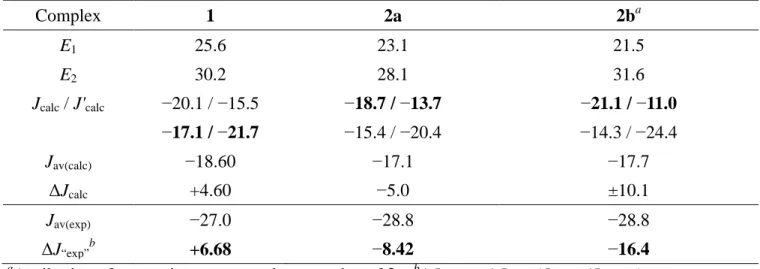
Table 3. Energies in cm-1 of the doublet states with respect to the quartet state Q (EQ = 0) for 1, 2a and

2b. Exchange coupling constants Jcalc and J'calc are extracted for the two types of isosceles magnetic

symmetries. For either symmetry, Jav(calc)and ΔJcalc are identical. In bold, the attribution based on the ab

initio expansions of the doublet states D0 and D1 wavefunctions as linear combination of Slater

determinants wavefunctions. Although indeterminate by magnetometry studies, “experimental” ΔJ

values can be estimated from ΔJcalc based on the Jav(exp)/Jav(calc) ratio.

Complex 1 2a 2ba E1 25.6 23.1 21.5 E2 30.2 28.1 31.6 Jcalc / J'calc −20.1 / −15.5 −18.7 / −13.7 −21.1 / −11.0 −17.1 / −21.7 −15.4 / −20.4 −14.3 / −24.4 Jav(calc) −18.60 −17.1 −17.7 ΔJcalc +4.60 −5.0 ±10.1 Jav(exp) −27.0 −28.8 −28.8 ΔJ“exp”b +6.68 −8.42 −16.4 a

Attribution of magnetic symmetry closest to that of 2a. bΔJ“exp” = ΔJcalc×(Jav(exp)/Jav(calc))

Another important conclusion, which is directly related to the rationalization of magnetic exchange strengths and to the symmetry of the molecular g-tensor (see below), concerns the magnetic orbitals of

the copper(II) ions. Qualitatively, such an analysis can be carried out using Addison’s criterion:55 if α

and β are the two largest L-M-L angles, the trigonality index τ5 = (α-β)/60 indicates an ideal square

pyramid for τ5 = 0, and an ideal trigonal bipyramid for τ5 = 1. E.g., in the case of 1 this criterion would

suggest that atoms Cu1 and Cu2 are closer to square pyramidal (τ5 = 0.22), whereas Cu3 is halfway

between square pyramid and tbp (τ5 = 0.57). On the other hand, inspection of the bond lengths would

also indicate that all three atoms are characterized by significantly compressed bonds along the N-Cu-N axes, and markedly elongated C-Cl bonds in the equatorial plane. This would suggest that all three

coordination polyhedra are better described as compressed tbp, which are known to endow CuII ions

with a 2

1

(d )_z ground state, making d_z2 their magnetic orbitals, instead of the d_x2_−y2 ones in square

pyramidal environments.

The ambiguity of this qualitative assessment is readily resolved by our calculations which confirm

that the magnetic orbitals are mostly of d_z2 character localized on copper(II) ions (Figure 3). One

13

not through the μ3-chlorides. The resulting poorly effective superexchange pathways can very well

rationalize the ferromagnetic interactions since they do not allow the development of the antiferromagnetic part of the exchange interaction.

Figure 3. Localized magnetic orbitals of 1 constructed from the CASSCF delocalized MOs. A similar picture holds for 2a and 2b.

EPR spectroscopy Single-crystal studies

To better understand the character of the quartet ground state in 1, single-crystal EPR studies were undertaken. EPR spectra were characteristic of zfs systems, and they were attributed to the ground S =

3/2 state, in perfect agreement with previously reported CH2Cl2 solution EPR spectra.22 No signals of

the excited doublets could be detected even at room temperature, probably due to fast relaxation. The spectra were characterized by broad lines due to unresolved hyperfine interactions. The amplitude of D

(~0.1 cm-1) was small enough for the EPR signals to fall nicely within the observable window of

X-band EPR wavelength (~0.3 cm-1), thus not necessitating the use of higher frequencies.

Experiments on oriented crystals were complicated by their low symmetry (triclinic P1, one independent molecule per unit cell) and the non-trivial relation between the molecular z-axis and the unit cell axes. Attempts to index single crystals and derive such relations were unsuccessful as the indexed faces could only be assigned to crystallographic planes with high Miller indices. These complications did not allow the confirmation of the absolute orientation of the magnetic z-axis within the crystal and, therefore, with respect to the molecular frame. However, they did allow the assessment of axiality of the EPR spectrum and the relative orientations of the g- and D-tensors.

In particular, it was possible to align a crystal by trial-and error, so that the molecule’s magnetic axis

was almost parallel to the Zeeman field (B0), as evidenced by the characteristic evenly-spaced 3-line

14

+1/2〉 transition. This is not permitted when z||B0, but acquires a non-zero probability amplitude due to

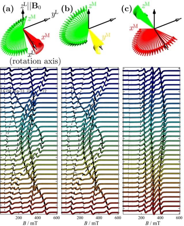
the non-parallel alignment of the magnetic axis to the Zeeman field. Rotations were performed from this orientation at 3° intervals between 0-180° (Figure 4, left), and then the crystal was turned by 90° around the two other orthogonal axes to carry out rotations around them (Figure 4, center and right). Due to this imperfect alignment, each series of rotations actually resulted in narrow precessions of the

molecular xM, yM, zM axes around the laboratory rotation axis (xL), with the magnetic field defining the

15

Figure 4. Top. Orientations of the molecular z-axis during 0-180° rotations a-c about the three orthogonal orientations. Bottom. Single-crystal X-band EPR spectra of 1 (black points) and their fits (colored lines) according to the models described in the text. For clarity, only every other spectrum is shown. Due to the imperfect alignment of the magnetic z-axis to the Zeeman field, the top and bottom

spectra in (a) and (b) are the closest to the ideal evenly spaced 3-line spectrum (z||B0). Fits to giant-spin

and multispin Hamiltonians are visually comparable and the latter are shown (solution II). The dashed lines are transition roadmaps, with their thickness indicative of the transition’s mean intensity. The

16

number pairs in panel (a) indicate the pairs of states involved in transitions: 1 ≡ |3/2, −3/2〉, 2 ≡ |3/2,

−1/2〉, 3 ≡ |3/2, +1/2〉, 4 ≡ |3/2, +3/2〉. The molecular orientation in the crystal is described by Euler angles {0, 16.0°, 0}. The crystal’s initial positions (top of panels) are described by the following Euler angles for each rotation: (a), {0, 0, 0} (by default); (b), {90°, 12.6°, 0}; (c), {0, 90°, 6.0°}. The

molecular orientations at those initial positions are described by Euler angles {177.6°, 16.0°, −177.7°},

{82.5°, 12.1°, 3.9°} and {47.5°, 74.7°, -7.6°}, respectively.

Initially the spectra were simulated using the giant-spin approximation, considering a zero-field split S = 3/2 system according to the Hamiltonian:

2 2 2

3/ 2 ˆ ˆ ˆ ˆ

ˆ _{( )}

z x y B i i

H =DS +E S −S +µ Hg S (6)

Attempts to fit to an axial (solution A) or rhombic (solution B) g-tensor yielded almost identical results (Table 4). Therefore, the former model was favored to avoid over-parametrization.

Consideration of an extremely small rhombicity of the D-tensor (E ~ 8×10-4 cm-1, E/D ~ 0.01)

improved the quality of the fits by ~11% in both cases (solutions C and D, respectively), a statistically significant improvement for the addition of just one parameter. Considering a small misalignment between the g- and D-tensors, in particular a relative rotation around the z-axis of ca. 11-12°, brought about a small (~1.5%) improvement to the fits, considered indicative (see below), though not quantitatively conclusive. Given the low symmetry of the crystal, fits to the giant spin model did not allow us to unequivocally demonstrate the tensor orientations within the crystal and molecular frames.

It is reasonably assumed that the gz and Dzz axes are normal to the triangle’s plane, an assumption that

was confirmed by implementation of the full multispin Hamiltonian analysis (see below).

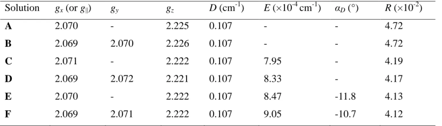
Table 4. Best-fit parameters to the single-crystal data based on the models described in the text. The R factor is Easyspin’s RMSD for the same data set.

Solution gx (or g||) gy gz D (cm-1) E (×10-4 cm-1) αD (°) R (×10-2) A 2.070 - 2.225 0.107 - - 4.72 B 2.069 2.070 2.226 0.107 - - 4.72 C 2.071 - 2.222 0.107 7.95 - 4.19 D 2.069 2.072 2.221 0.107 8.33 - 4.17 E 2.070 - 2.222 0.107 8.47 -11.8 4.13 F 2.069 2.071 2.222 0.107 9.05 -10.7 4.12

17

Then, EPR spectra were analyzed using the full multispin Hamiltonian to grasp the origin of the zfs. Such Hamiltonian accounts for isotropic, DM, dipolar and anisotropic interactions, as well as for the local gi-tensor orientations.

To minimize the number of free variables, an isosceles isotropic Hamiltonian term, with J13 = J23 = J

= −25.9 cm-1 and J12 = J' = −29.1 cm-1 was considered. This assignment was based on the Jav value

derived from magnetic susceptibility studies (Jav = −27.0 cm-1, Table 2), and on the ΔJ value derived

from consideration of ab initio calculations. For that latter parameter, as the calculated Jav value

exhibited some deviation from the experimentally determined one, the size of ΔJ was calculated by

scaling accordingly, and fixed to |ΔJexp| = |ΔJcalc|×(Jav(exp)/Jav(calc)) = 6.68 cm-1. As for its sign, which

determines the type of isosceles magnetic symmetry (|J| > |J'| vs. |J| < |J'|), this was determined by the

reading of the ab initio wavefunctions of doublets D0 and D1, leading to a value of ΔJexp = +6.68 cm-1.

In calculating the dipolar term, the general expression for the interaction matrix was applied, as

(

)(

)

T T T

3

dip

ij = i j− i ⋅ ij ij⋅ j 

D ρg gρ g g (7), where ρij = rij/|rij| is the unit vector between sites i and j. This is

a 3×3 interaction matrix whose structure is a function of the relative orientations of the two g-tensors, and becomes symmetric when they are parallel. In the point-dipole approximation of isotropic spins, it is diagonal and traceless, and the interaction energy is only determined by the intersite distance. This is a satisfactory approximation in the case of organic radicals separated by large distances. However, in the case of highly anisotropic metal ions in close proximity, g-tensor misalignments become important.

Analytical expressions have been derived in the reference frame of one of the spins (g1 by convention,

whose tensor is therefore diagonal).46,47 Whereas this may be a useful convention for dinuclear

complexes (or radical pairs), the use of the molecular frame of reference is a more convenient convention for higher nuclearity systems.

We opted for the latter convention and defined the principal axes of the local g-tensors with respect to the molecular frame of reference. In doing so, we took into account the compressed tbp coordination

sphere of the copper(II) ions, which gives rise to magnetic orbitals of d_z2 character, as already

mentioned. This coordination geometry reverses the g-tensor values to g⊥ > g||56–61 an observation taken

into consideration during the fits.

According to the above, we arranged their tensors so that their principal z-axes coincide with the

idealized N-Cu-N directions, with the Euler angles {α, β, γ} being {π, -π/2, γ1}, {-π/3, -π/2, γ2} and

{π/3, -π/2, γ3} for sites i = 1, 2 and 3, respectively, with respect to the molecular frame (Figure 5 and

18

convention selected for Euler angles is zyz', as used by Easyspin functions). This can intuitively be associated, though it does not strictly coincide (see below), with the angular deviation of the terminal

chlorides from the in-plane position. We then calculated the respective rotation matrices R(α, β, γ)

which transform the tensors to the molecular frame (M-frame) through the relation:

T

( , , )α β γ ( , , )α β γ

′ = ⋅ ⋅

g R g R (8)

We then used ′g to calculate the interaction matrices in the molecular frame. In that frame, the

vectors ρ12, ρ13 and ρ23 were described by Euler angles {π/3 0 0}, {-π/3 0 0} and {π/2 0 0}, respectively.

Due to the presence of antisymmetric elements in the dip

ij

D tensors when expressed in the M-frame, we

decomposed them to their symmetric and antisymmetric parts to find their real eigenvalues:

(

)

(

)

dip sym dip dip T

ij ij ij

dip anti dip dip T

ij ij ij = + = − D D D D D D       (9) (10)

and used the symmetric part for the plots of D . dip_M

A comment should be made regarding the validity of this model. It is known that spin delocalization, e.g. such as observed in unsaturated radical systems, can cause important deviations from the

point-dipole approximation.62 In our case, calculations show that orbitals located on the metal centers are of d

character and are not delocalized over the molecule. Indeed, the HOMO orbital is antibonding between the metals and the pyrazole nitrogen atoms (Figure 3). Another possible source of deviation from the point-dipole model is the redistribution of spin density due to magnetic exchange, which influences the

spin expectation values 〈Ŝiz〉, i.e. the spin density on each site.40,54 For the spin Hamiltonian parameters

of 1, calculations show that in the ground state |ST = 3/2, MS = −3/2〉, the three spin centers are

equivalent, with 〈Ŝ1z〉 = 〈Ŝ2z〉 = 〈Ŝ3z〉 = −0.5, which further reinforces the validity of the point-dipole

approximation. Similarly, ab initio calculations show equal spin densities on the three sites.

Turning to the anisotropic interactions, in the general form of the interaction tensor as expressed in

Equation (3), this is defined by five independent variables, i.e. Jij Jij

αβ ₌ βα

(α, β = x, y, z), with

zz xx yy ij ij ij

J = −J −J being a dependent variable (p. 63 of reference 63), and its eigenvectors define the

reference frame of the pairwise anisotropic exchange interaction. A perfectly equilateral symmetry for this tensor (i.e., ₁₂ani = ₁₃ani = ₂₃ani

D D D in the respective frames) introduces an additional consideration: such

a model cannot reproduce possible rhombicities stemming from anisotropic interactions, since the tensorial sum cancels them out. Indeed, as was shown on the basis of our numerical simulations, the total D_Mani tensor is then characterized by J_M(ani xx) =J_M(ani yy) , meaning that the coupled ground state

19

corresponds to a purely axial system, as far as anisotropic exchange is concerned, since

( 1 ( ) , 1 ( ( ) ( ) )

2 2

ani ani zz ani xx ani yy

M M M M

D = J E= J −J ), even in the presence of rhombic pairwise anisotropic

terms (pp. 653-654 of reference 63).

With such a model, the only rhombicity in the quartet state is due to dipolar interactions, since the rij

distances and γi angles (see below) break the structural symmetry. However, it cannot account for

rhombicities stemming from anisotropic exchange. One way to circumvent this deficiency, is to relax the constraint of equilateral symmetry in the anisotropic exchange term, introducing 3 × 5 = 15 (instead of just 5) independent variables into the model; However, this leads to overparametrization. To do so with the minimum amount of additional parameters, we initially sought to scale one of the three tensors

as D_13,23ani =aD and use a as a free variable (5 + 1 = 6 free variables). However, this strategy was not ₁₂ani

successful. Finally, considering D₁₂ani ≠D₁₃ani =D (5 + 5 = 10 free variables), significantly improved ₂₃ani

the agreement to the data, but due to the important number of additional free variables we remain cautious as to the physical significance of the magnitude of each of these variables.

To summarize, the multispin Hamiltonian matrix considered was:

3 1 3 2 3 1 3 , 1 2 3 3 1 12 2 3 , (1,3),(2,3) , 1 1 ˆ ˆ ˆ ˆ ˆ ˆ ˆ ˆ ˆ _{( ) ( )} ˆ ˆ ˆ ˆ ˆ ˆ ˆ ij i j i j

ani ani dip

i ij j i ij j i i i j i j ij i H J J r β _β = = = = ′ = ⋅ + ⋅ + ⋅ + × + ′ + ⋅ ⋅ + ⋅ ⋅ + ⋅ ⋅ +

∑

∑

∑

∑

but its physical meaning can confidently be established only in the case of D′ =ani D . ani

The crystal structure was used to fix the intermetallic distances and to provide an initial estimate of the g-tensor orientations. Only three free variables were introduced in this part of our model, in

particular those describing the “twist” of the individual gi⊥ axes with respect to the triangle plane. The

principal values of the g-tensors were considered equal for all three ions, requiring the introduction of only three variables. Five (or ten, see above) variables were considered for the general expression of the anisotropic exchange interactions.

Similarly, three additional variables would be required for DM interactions; although the anions do

not contain crystallographically imposed C3 axes and σh planes, the molecular symmetry is such that

can be approximated by a pseudo-D3h point group. Following the Moriya rules, this allows to consider

Gz as the principal component of the DM interaction matrix. However, these variables were finally

20

In all, eleven (or sixteen) free variables were considered for the Hamiltonian, plus four more to describe the orientation of the molecule in the crystal and of the crystal in the laboratory frame, and two to describe the intrinsic line widths (Gaussian and Lorentzian). These seventeen (or twenty-two) fitting parameters compare quite well with the 183 (= 61 × 3) single-crystal spectra which formed our data set.

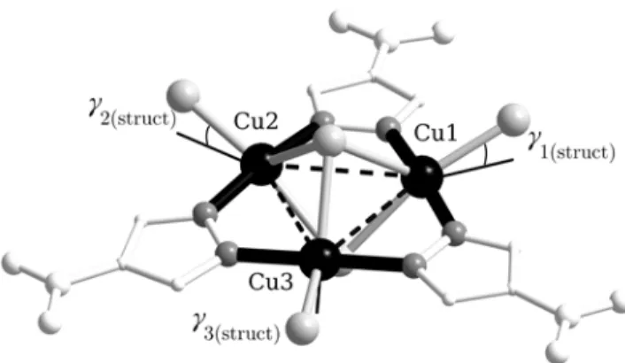
Figure 5. Structure of the anion of 1 showing the intramolecular superexchange interactions (dashed lines). The axial compression axes of the trigonal bipyramids are indicated by black thick bonds,

whereas the equatorial planes are indicated by grey thin bonds. The angles γ1-3 indicate the deviation of

the Cu-Clterm bonds from the triangle plane.

Initial attempts to fit the spectra by only considering the dipolar interactions yielded a partial account of the zfs of the ground state, confirming that DM and/or anisotropic interactions need also be

considered. Our first attempt considered DM interactions based on the predictions of Belinsky29

However, no discernible zfs was induced by any combination of Gx/y/z elements. Simulations showed

that the only way to introduce zfs through DM interactions was to reverse one of the G pseudovectors, i.e. assume that [G12x G12y G12z] = [G13x G13y G13z] = −[G23x G23y G23z] (expressed in the local interaction

frames), for which, however, no plausible rationale could be found.

We therefore turned to anisotropic interactions as a zfs-inducing term. A series of fits demonstrated that J and _ijxx J_ijyy(expressed in the local ij-reference frames) were the leading parameters in determining the zfs and that several combinations achieved very good agreement with experimental data. Indicative

fits with values of ca. -0.045 cm-1 are shown on Table 5. The total g_M and Dani_M were calculated

through the following relations for an ST = 3/2 state stemming from three Si = 1/2 spins (Table 4.4 of

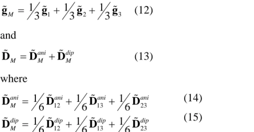
21 1 2 3 1 1 1 3 3 3 M = + + g g g g (12) and ani dip M = M + M D D D (13) where 12 13 23 12 13 23 1 1 1 6 6 6 1 1 1 6 6 6

ani ani ani ani

M

dip dip dip dip

M = + + = + + D D D D D D D D         (14) (15)

and where each individual tensor is expressed in the M-frame for the addition.

The various models tested indicate that a ~10% improvement to the fit quality was obtained by

introducing the rotations of the local gi-tensors as free variables (solution II). Additionally, breaking the

equilateral symmetry of the anisotropic interactions by introducing an independent D interaction ₁₂ani

matrix (solution III) affords a further improvement of ~11% over solution II. Although this is to be statistically expected from the introduction of five free variables, we note that this solution better reproduces the rhombic zfs term that was found during fits to the giant spin model (see Table 4).

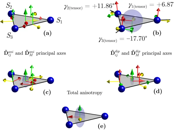
Figure 6 shows the orientations of the various tensors for solution II of Table 5, in the reference frames in which each is diagonal. It should be noted that these tensors are not diagonal in the same reference frames, and that their principal axes (eigenvectors) do not perfectly coincide with any of the M and ij frames. For comparison, the respective plots for solutions I (Figures S1) and III (Figure S2) are given in the Supporting Information.

22

Figure 6. Illustration of tensor elements based on best-fit parameters of solution II (axis color code: x = red, y = yellow, z = green). (a). Principal reference frames definitions: molecular (M) on the triangle center, and interaction (ij) on the midpoints of the interspin vectors. (b-d). Principal axes of local and molecular g-tensors (b), local and molecular anisotropic exchange tensors (c) and dipolar interaction tensors (d) as determined from fits to single-crystal data. (e). Local axes of the total anisotropy tensor derived from the sum of the anisotropic and dipolar parts. The blue semi-transparent ellipsoids illustrate the relative sizes of the eigenvalues along each axis, hence the axiality of each tensor. For

, ,

ani dip

M M M

D D D they are in the same scale.

These results are in very good agreement with the fits carried out based on a giant-spin model. They corroborate our initial assumption that the principal z-components of g and D axes are normal to the triangle plane and practically collinear, with a misalignment mainly regarding a rotation around their common z-axis.

23

Our results indicate an almost axial g-tensor, and reproduce faithfully the results of the giant-spin solution C. They also yield an average g value g_av = (g_x2+g_y2+g_z2) / 3= 2.124, i.e. remarkably close to the value of 2.125 derived from magnetic susceptibility data (Table 2). They also rationalize the fact

that although the local g-tensors have an inversed order (gi|| < gi⊥) the coupled system exhibits a

“normal” order for CuII (gM|| > gM⊥). Indeed, as the local (large) gx components are projected onto the

molecular z-axis, they yield a large gzM due to their out-of-plane orientations. As far as the “twist”

angles are concerned, the fits showed a remarkable sensitivity to the values of these parameters, and a clear preference for a particular local error minimum. We should note, however, that these angles do not coincide with any structural parameters, the most intuitive of which would be the angular deviation

of the Cu-Clterminal bond out the Cu3 plane. The only empirical correlation we established is that the

local g-tensors are rotated around their z-axes by ca. 15-30° with respect to the Cu-Clterminal bond (see

γi(struct) – γi(tensor) in Table 6).

The two series of fits (giant-spin vs multispin model) are also coherent with respect to the improvement brought about by full inclusion of rhombic contributions of anisotropic exchange, as they closely reproduce the sizes of D and E of the ground state zfs. The non-uniqueness of solutions for anisotropic interactions is attributed to the triangular symmetry of the system which results in different parameter sets yielding similar tensorial sums.

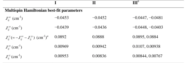
Table 5. Best-fit parameters according to different models and derived parameters of the coupled-system tensors. The different solutions illustrate the effect of inclusion of g-tensor rotations and of an isosceles distortion of the anisotropic exchange to the quality of the fits. Figures in bold italics indicate fixed values.

I II IIIb

Multispin Hamiltonian best-fit parameters

xx ij J (cm-1) −0.0453 −0.0452 −0.0447, −0.0481 yy ij J (cm-1) −0.0439 −0.0436 −0.0448, −0.0403 ( ) zz xx yy ij ij ij J = −J −J (cm-1)a 0.0892 0.0888 0.0895, 0.0884 xy ij J (cm-1) 0.00969 0.00942 0.0107, 0.00938 xz ij J (cm-1) 0.00953 0.00836 0.00844, 0.00767

24 yz ij J (cm-1) 0.00867 0.00909 0.00941, 0.00897 gix 2.226 2.226 2.225 giy 2.126 2.126 2.125 giz 2.014 2.015 2.013 γ1 (°) 0 6.87 9.25 γ2 (°) 0 11.86 11.82 γ3 (°) 0 −17.70 −23.36 RMSD 4.35×10-2 3.90×10-2 3.49×10-2

Derived spin-Hamiltonian parameters for exchange-coupled quartet state

Dani, Eani (cm-1) 0.0670, 0 0.0666, 0 0.0667, −7.17×10-4 Ddip, Edip (cm-1) 0.0410, −5.09×10-4 0.0408, −4.83×10-4 0.0406, −4.72×10-4 Dtot, Etot (cm-1) 0.108, −5.09×10-4 0.107, −4.83×10-4 0.107, −1.12×10-3 gMx 2.070 2.072 2.071 gMy 2.070 2.072 2.073 gMz 2.227 2.223 2.220 a

Dependent variable. bDouble values for the anisotropic exchange parameters refer to tensor elements

13,23, 12

Jαβ Jαβ(α, β = x, y, z).

Table 6. Comparison between the out-of-plane deviation of the terminal chlorides with the “twist” angle of the local gi-tensors around the giz local axes (from solution II).

i-ion γi(struct) (°) γi(tensor) (°) γstruct – γtensor (°)

1 −21.01 +6.87 −27.88

2 −19.67 +11.86 −31.53

3 +0.64 −17.70 +17.06

A final comment is in order regarding the signs of D and E: During the fitting attempts, simulations were carried out on an extensive number of parameter combinations for the anisotropic exchange interaction matrix. Of all these combinations, none led to a negative value of D after eigendecomposition. On the one hand, this is in agreement with the findings of high-frequency EPR studies previously reported on the related complex (Bu4N)2[Cu3(μ3-Cl)2(pz)3Cl3], and which concluded

25

symmetry of the problem does not allow for D < 0, at least when dipolar and anisotropic interactions are considered. A mathematical proof to that effect is beyond the scope of the current work, so, this conclusion is offered on a tentative basis.

With regard to the sign of E, this is determined during the diagonalization of the full interaction matrix

2 3

3 , 1

HDvV DMI ani dip

ij ij ij ij

i j rij

β

=

=

∑

J D D D D , whose individual terms are given Equations 1-4 and 7.

The order of eigenvalues in the diagonalized matrix D = VTJV is related to the ordering of matrix V

containing the eigenvectors as columns. By choosing an ascending order (Dxx < Dyy < Dzz), the x and y

eigenvectors in V may be swapped in low rhombicity (Dxx ~ Dyy) systems. This a typical situation in zfs

systems, where the sign of E bears no physical meaning, other than signifying the handedness of the reference frame.

Powder and solution EPR spectra

Single-crystal EPR data are not always easily available, nor is their analysis always straightforward. We were therefore interested to assess whether we could derive useful conclusions as to the magnetic

structures of ferromagnetic CuII3 pyrazolates from powder or frozen solution data. Accordingly, EPR

spectra were collected from powders and frozen CH2Cl2 solutions of 1-4.

Powder spectra of complexes 1, 2 and 4 exhibited characteristic zfs spectra, attributed to their S = 3/2 ground states. Preliminary fits with a simple giant-spin model yielded excellent results assuming

collinear g and D, with solid-state gav values for 1-3 (2.121, 2.164, 2.115, respectively, Table 7)

following closely the ones determined from magnetic susceptibility data, even reproducing the higher g-value of 2 (Table 2). These fits revealed consistent D values of ca. 0.08-0.11 cm-1 in the solid state

and 0.04-0.1 cm-1 in frozen solutions. Except for the powder spectrum of 1, all other spectra required

the introduction of small D-strains to satisfactorily fit the data, using Easyspin’s built-in function. This is attributed to distributions of magnetic conformers for the frozen solution spectra, and to the presence of more than one molecules in the asymmetric units of 2 and 3 (two and four, respectively) in the solid state spectra.

A salient exception was the low-melting24 3, which was characterized by an exceptionally small zfs

and broad lines which masked the characteristic zfs patterns, particularly for a molten and re-cooled frozen glass. For that particular spectrum, the smearing out of any distinctive patterns precluded any meaningful fit, and only a tentative simulation was carried out. In turn, the frozen solution spectrum was characterized by somewhat narrower lines, which allowed simulation taking into account a Gaussian distribution of the D parameter. This was the lowest among the complexes studied here. In the

26

context of the giant spin analysis, a custom-made D-strain model was applied, considering a combination of Gaussian and Lorentzian distributions of the D parameter, as previously implemented in other systems.64,65

Table 7. Best-fit parameters from fits of powder and frozen solution EPR spectra of complexes 1-4 to a

giant-spin model. The σG/L values are the Gaussian and Lorentzian contributions to the intrinsic line

widths, and σDG is the Gaussian line width of the D-strain.

Complex State T / K |D| (cm-1) g|| g⊥ σG/σL (mT) σDG (cm-1) gav 1 Powder 290 0.105 2.213 2.074 25.4/0 0 2.121 CH2Cl2 4.2 0.096 2.212 2.085 21.0/0 0.043 2.128 2 Powder 290 0.079 2.290 2.098 30/14 0.041 2.164 CH2Cl2 4.2 0.050 2.190 2.088 17.7/0 0.017 2.123 3 Powder 290 0.037 2.222 2.060 20/20 0 2.115 Molten 290 ~0 ~2.10 ~2.10 0/50 CH2Cl2 4.2 0.043 2.247 2.088 14.6/6.8 0.033/0.017 2.142 4 Powder 290 0.088 2.226 2.080 37.8/0 0.035 2.130 CH2Cl2 4.2 0.059 2.185 2.091 17.5/0 0.040 2.123

27

Figure 7. Powder (290 K) and frozen CH2Cl2 solution (4.2 K) X-band EPR spectra of 1-4 and fits

based on a giant-spin Hamiltonian, assuming axial zfs and D-strain effects. The D-strain effect for the frozen solution spectrum of complex 3 was carried out using a custom distribution function, shown in the inset.

28

Subsequently, we attempted to interpret our powder and solution data with a simplified version of the previously employed multispin Hamiltonian. In particular, we considered axial local g-tensors and, accordingly, we neglected their “twist” angles. Moreover, we neglected the pairwise rhombicities of anisotropic interactions by considering a minimal form of the anisotropic exchange interaction matrix:

1 / 2 0 0 0 1 / 2 0 0 0 1 ani zz ij Jij −     = _ − _     D (16)

According to our methodology, dipolar interactions were calculated from structural parameters

appropriate to this level of precision, namely the rij distances, since the g-tensor orientations were

considered indeterminate from powder data. This cautious approach was validated by the subsequent

observation that even the gi|| and gi⊥ values were indeterminate in some data sets, obliging us to

constrain them to physically meaningful values for copper(II) ions (i.e. gi > 2). The results of the fits

are summarized in Table 8.

During our fitting attempts of the powder data of 1, we observed that two solutions give good fits,

one with Jzz ~ +0.085 cm-1, and another with Jzz ~ –0.19 cm-1. However, eigenvalue analysis revealed

that the latter corresponds to physically non-meaningful parameters with E/D ~ 1, whereas eigenvector analysis indicates that in that solution the principal anisotropy axis lies in the triangle plane (Figure S3). This solution was therefore discarded, while that observation was then used to assess subsequent fits to the data of the other complexes. The results for 1 were in close agreement with the single-crystal fits,

yielding practically the same Jzz parameter, thus validating our methodology (cf. Table 5 and Table 8).

Globally, fits for all complexes were of good quality (Figure 9), although somewhat inferior to that of the fits to a giant-spin model (Figure 7) as we did not consider strain effects. Moreover, the derived D parameters for the exchange-coupled quartets were very close to the ones derived from the giant-spin model (cf. Table 7 and Table 8). Taken together, these observations further validated our approach. It should also be noted that the dipolar contributions to zfs all fell within a very narrow range

(0.038-0.039 cm-1), to be expected from the very similar structures of the complexes.

Table 8. Best-fits parameters to the powder EPR spectra of complexes 1-4 using the simplified version

of the full multispin Hamiltonian. a Figures in bold italics indicate fixed values.

Complex Multispin Hamiltonian parameters Derived parameters for quartet-state gi|| gi⊥ σG/σL (mT) Jzz (cm-1) Ddip (cm-1) Dani (cm-1) D (cm-1) gM|| gM⊥ D ani /D (%)

29 1 2.001 2.178 15.8/10.4 0.0850 0.0393 0.0637 0.103 2.181 2.091 62 2ab 2.071 2.179 18.9/25.3 0.0481 0.0380 0.0360 0.0741 2.179 2.125 49 2bb 2.071 2.179 18.9/25.3 0.0479 0.0382 0.0359 0.0741 2.179 2.125 49 3c 2.092 2.155 24.3/0 0 0.0387 0 0.0387 2.155 2.123 0 4d 2.001 2.161 25.3/14/8 0.0663 0.0388 0.0497 0.0885 2.166 2.084 56 a

Values of Jav(exp) and ΔJ“exp” for 1, 2a and 2b taken from Table 3. In the absence of calculations for 3

and 4, the values of 1 were used. bDipolar contributions calculated using rij distances of the respective

molecule. cFrozen solution spectrum (CH2Cl2, 4.2 K), assuming r12 = r13 = r23 = 3.4 Å. dThere are four

molecules in the asymmetric unit and for simplicity calculations assume a single molecule with r12 =