RESEARCH OUTPUTS / RÉSULTATS DE RECHERCHE
Author(s) - Auteur(s) :
Publication date - Date de publication :
Permanent link - Permalien :
Rights / License - Licence de droit d’auteur :
Bibliothèque Universitaire Moretus Plantin
Institutional Repository - Research Portal
Dépôt Institutionnel - Portail de la Recherche
researchportal.unamur.be
University of Namur
Test them all, is it worth it? Assessing configuration sampling on the JHipster Web
development stack
Halin, Axel; Nuttinck, Alexandre; Acher, Mathieu; Devroey, Xavier; Perrouin, Gilles; Baudry,
Benoit
Published in:
Empirical Software Engineering DOI:
10.1007/s10664-018-9635-4
Publication date: 2019
Link to publication
Citation for pulished version (HARVARD):
Halin, A, Nuttinck, A, Acher, M, Devroey, X, Perrouin, G & Baudry, B 2019, 'Test them all, is it worth it? Assessing configuration sampling on the JHipster Web development stack', Empirical Software Engineering , vol. 24, no. 2, pp. 674-717. https://doi.org/10.1007/s10664-018-9635-4
General rights
Copyright and moral rights for the publications made accessible in the public portal are retained by the authors and/or other copyright owners and it is a condition of accessing publications that users recognise and abide by the legal requirements associated with these rights. • Users may download and print one copy of any publication from the public portal for the purpose of private study or research. • You may not further distribute the material or use it for any profit-making activity or commercial gain
• You may freely distribute the URL identifying the publication in the public portal ?
Take down policy
If you believe that this document breaches copyright please contact us providing details, and we will remove access to the work immediately and investigate your claim.
(will be inserted by the editor)
Test them all, is it worth it? Assessing configuration sampling
on the JHipster Web development stack
Axel Halin · Alexandre Nuttinck · Mathieu Acher · Xavier Devroey · Gilles Perrouin · Benoit Baudry
Received: date / Accepted: date
Abstract Many approaches for testing configurable soft-ware systems start from the same assumption: it is impossible to test all configurations. This motivated the definition of variability-aware abstractions and sam-pling techniques to cope with large configuration spaces. Yet, there is no theoretical barrier that prevents the exhaustive testing of all configurations by simply enu-merating them if the effort required to do so remains acceptable. Not only this: we believe there is a lot to be learned by systematically and exhaustively testing a configurable system. In this case study, we report on the first ever endeavour to test all possible configura-tions of the industry-strength, open source configurable software system: JHipster, a popular code generator for web applications. We built a testing scaffold for the 26,000+ configurations of JHipster using a cluster of 80 machines during 4 nights for a total of 4,376 hours (182 days) CPU time. We find that 35.70% configura-tions fail and we identify the feature interacconfigura-tions that cause the errors. We show that sampling strategies (like
A. Halin, G. Perrouin (FNRS research associate) PReCISE, NaDI, Faculty of Computer Science University of Namur, Belgium
E-mail: gilles.perrouin@unamur.be A. Nuttinck
CETIC, Belgium
E-mail: alexandre.nuttinck@cetic.be M. Acher
IRISA, University of Rennes I, France E-mail: mathieu.acher@irisa.fr X. Devroey
SERG, Delft University of Technology, The Netherlands E-mail: x.d.m.devroey@tudelft.nl
B. Baudry
KTH Royal Institute of Technology, Sweden E-mail: baudry@kth.se
dissimilarity and 2-wise): (1) are more effective to find faults than the 12 default configurations used in the JHipster continuous integration; (2) can be too costly and exceed the available testing budget. We cross this quantitative analysis with the qualitative assessment of JHipster’s lead developers.
Keywords Configuration sampling · variability-intensive system · software testing · JHipster · case study
1 Introduction
Configurable systems offer numerous options (or fea-tures) that promise to fit the needs of different users. New functionalities can be activated or deactivated and some technologies can be replaced by others for address-ing a diversity of deployment contexts, usages, etc. The engineering of highly-configurable systems is a stand-ing goal of numerous software projects but it also has a significant cost in terms of development, maintenance, and testing. A major challenge for developers of con-figurable systems is to ensure that all combinations of options (configurations) correctly compile, build, and run. Configurations that fail can hurt potential users, miss opportunities, and degrade the success or reputa-tion of a project. Ensuring quality for all configurareputa-tions is a difficult task. For example, Melo et al. compiled 42,000+ random Linux kernels and found that only 226 did not yield any compilation warning [54]. Though for-mal methods and program analysis can identify some classes of defects [14, 77] – leading to variability-aware testing approaches (e.g., [43, 44, 56]) – a common prac-tice is still to execute and test a sample of (represen-tative) configurations. Indeed, enumerating all configu-rations is perceived as impossible, impractical or both.
While this is generally true, we believe there is a lot to be learned by rigorously and exhaustively testing a configurable system. Prior empirical investigations (e.g., [52, 70, 71]) suggest that using a sample of config-urations is effective to find configuration faults, at low cost. However, evaluations were carried out on a small subset of the total number of configurations or faults, constituting a threat to validity. They typically rely on a corpus of faults that are mined from issue tracking systems. Knowing all the failures of the whole config-urable system provides a unique opportunity to accu-rately assess the error-detection capabilities of sampling techniques with a ground truth. Another limitation of prior works is that the cost of testing configurations can only be estimated. They generally ignore the exact computational cost (e.g., time needed) or how difficult it is to instrument testing for any configuration.
This article aims to grow the body of knowledge (e.g., in the fields of combinatorial testing and software product line engineering [15, 27, 32, 52, 53, 71]) with a new research approach: the exhaustive testing of all configurations. We use JHipster, a popular code genera-tor for web applications, as a case study. Our goals are: (i) to investigate the engineering effort and the com-putational resources needed for deriving and testing all configurations, and (ii) to discover how many failures and faults can be found using exhaustive testing in or-der to provide a ground truth for comparison of diverse testing strategies. We describe the efforts required to distribute the testing scaffold for the 26,000+ configu-rations of JHipster, as well as the interaction bugs that we discovered. We cross this analysis with the qualita-tive assessment of JHipster’s lead developers. Overall, we collect multiple sources that are of interest for (i) re-searchers interested in building evidence-based theories or tools for testing configurable systems; (ii) practition-ers in charge of establishing a suitable strategy for test-ing their systems at each commit or release. This ar-ticle builds on preliminary results [25] that introduced the JHipster case for research in configurable systems and described early experiments with the testing in-frastructure on a very limited number of configurations (300). In addition to providing a quantitative assess-ment of sampling techniques on all the configurations, the present contribution presents numerous qualitative and quantitative insights on building the testing infras-tructure itself and compares them with JHipster de-velopers’ current practice. In short, we report on the first ever endeavour to test all possible configurations of the industry-strength open-source configurable soft-ware system: JHipster. While there have been efforts in this direction for Linux kernels, their variability space forces to focus on subsets (the selection of 42,000+
ker-nels corresponds to one month of computation [54]) or to investigate bugs qualitatively [1, 2]. Specifically, the main contributions and findings of this article are:
1. a cost assessment and qualitative insights of engi-neering an infrastructure able to automatically test all configurations. This infrastructure is itself a con-figurable system and requires a substantial, error-prone, and iterative effort (8 man*month);
2. a computational cost assessment of testing all con-figurations using a cluster of distributed machines. Despite some optimizations, 4,376 hours (∼182 days) CPU time and 5.2 terabytes of available disk space are needed to execute 26,257 configurations; 3. a quantitative and qualitative analysis of failures
and faults. We found that 35.70% of all configura-tions fail: they either do not compile, cannot be built or fail to run. Six feature interactions (up to 4-wise) mostly explain this high percentage;
4. an assessment of sampling techniques. Dissimilar-ity and t-wise sampling techniques are effective to find faults that cause a lot of failures while requiring small samples of configurations. Studying both fault and failure efficiencies provides a more nuanced per-spective on the compared techniques;
5. a retrospective analysis of JHipster practice. The 12 configurations used in the continuous integration for testing JHipster were not able to find the defects. It took several weeks for the community to discover and fix the 6 faults;
6. a discussion on the future of JHipster testing based on collected evidence and feedback from JHipster’s lead developers;
7. a feature model for JHipster v3.6.1 and a dataset to perform ground truth comparison of configura-tion sampling techniques, both available at https: //github.com/xdevroey/jhipster-dataset. The remainder of this article is organised as follows: Section 2 provides background information on sampling techniques and motivates the case; Section 3 presents the JHipster case study, the research questions, and methodology applied in this article; Section 4 presents the human and computational cost of testing all JHip-ster configurations; Section 5 presents the faults and failures found during JHipster testing; Section 6 makes a ground truth comparison of the sampling strategies; Section 7 positions our approach with respect to stud-ies comparing sampling strategstud-ies on other configurable systems; Section 8 gives the practitioners point of view on JHipster testing by presenting the results of our in-terview with JHipster developers; Section 9 discusses the threats to validity; and Section 10 wraps up with conclusions.
2 Background and Related Work
Configurable systems have long been studied by the Software Product Line (SPL) engineering community [6, 65]. They use a tree-like structure, called feature model [40], to represent the set of valid combinations of options: i.e., the variants (also called products). Each option (or features1) maybe decomposed into sub-features and additional constraints may be specified amongst the different features.
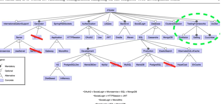
For instance, Figure 1 presents the full feature model of JHipster. Each JHipster variant has a Generator op-tion that may be either a Server, a Client, or an Appli-cation; may also have a Database that is SQL or Cas-sandra or MongoDB; etc. Additional constraints specify for instance that SocialLogin may only be selected for Monolithic applications.
2.1 Reverse Engineering Variability Models
The first step required to reason on an existing con-figurable system is to identify its variability. There are some approaches in the literature that attempt to ex-tract variability and synthesize a feature model. For example, She et al. devised a technique to transform the description language of the Linux kernel into a rep-resentative feature model [73]. The inference of parent-child relationships amongst features proved to be prob-lematic as the well as the mapping of multi-valued op-tions to boolean features. As a result, feature models extracted with such a technique have to be further val-idated and corrected [28]. Abbasi et al. [3] designed an extraction approach that first look for variability patterns in web configurator tools and complete ex-tracted information using a web crawler. In this case, the feature model is not synthesised. Indeed, static anal-ysis has been largely used to reason about configura-tion opconfigura-tions at the code level (e.g., [55, 67]). Such tech-niques often lie at the core of variability-aware testing approaches discussed below. As we will detail in our study, the configurator implementation as well as vari-ation points of JHipster are scattered in different kinds of artefacts, challenging the use of static and dynamic analyses. As a result, we rather used a manual approach to extract a variability model. Though automated vari-ability extraction can be interesting to study JHipster evolution over the long term, we leave it out of the scope of the present study.
1 In the remaining of this paper, we consider features as
units of variability: i.e., options.
2.2 Testing a Configurable System
Over the years, various approaches have been devel-oped to test configurable systems [16, 20, 50]. They can be classified into two strategies: configurations sampling and variability-aware testing. Configuration sampling approaches sample a representative subset of all the valid configurations of the system and test them in-dividually. Variability-aware testing approaches instru-ment the testing environinstru-ment to take variability infor-mation and reduce the test execution effort.
2.2.1 Variability-aware testing
To avoid re-execution of variants that have exactly the same execution paths for a test case, Kim et al. and Shi et al. use static and dynamic execution analysis to collect variability information from the different code artefacts and remove relevant configurations accord-ingly [44, 74].
Variability-aware execution approaches [9,43,56] in-strument an interpreter of the underlying programming language to execute the tests only once on all the vari-ants of a configurable system. For instance, Nguyen et al. implemented Varex, a variability-aware PHP inter-preter, to test WordPress by running code common to several variants only once [56]. Alternatively, instead of executing the code, Reisner et al. use a symbolic execu-tion framework to evaluate how the configuraexecu-tion op-tions impact the coverage of the system for a given test suite [69]. Static analysis and notably type-checking has been used to look for bugs in configurable soft-ware [41, 42]. A key point of type-checking approaches is that they have been scaled to very large code bases such as the Linux kernel.
Although we believe that JHipster is an interest-ing candidate case study for those approaches, with the extra difficulty that variability information is scat-tered amongst different artefacts written in different languages (as we will see in Section 4.1), they require a (sometimes heavy) instrumentation of the testing envi-ronment. Therefore, we leave variability-aware testing approaches outside the scope of this case study and fo-cus instead on configuration sampling techniques that can fit into the existing continuous integration environ-ment of JHipster developers (see Section 8.1).
2.2.2 Configurations sampling
Random sampling. This strategy is straightforward: se-lect a random subset of the valid configurations. Arcuri et al. [8] demonstrate that, in the absence of constraints between the options, this sampling strategy may out-perform other sampling strategies. In our evaluation,
Fig. 1 JHipster reverse engineered feature model (only an excerpt of cross-tree constraints is given).
random sampling serves as basis for comparison with other strategies.
T-wise sampling. T-wise sampling comes from Combi-natorial Interaction Testing (CIT), which relies on the hypothesis that most faults are caused by undesired in-teractions of a small number of features [46]. This tech-nique has been adapted to variability-intensive systems for more than 10 years [15,49]. A t-wise algorithm sam-ples a set of configurations such that all possible t-usam-ples of options are represented at least once (it is generally not possible to have each t-uples represented exactly once due to constraints between options). Parameter t is called interaction strength. The most common t-wise sampling is pairt-wise (2-t-wise) [15, 32, 36, 61, 79]. In our evaluation, we rely on SPLCAT [38], an efficient t-wise sampling tool for configurable systems based on a greedy algorithm.
Dissimilarity sampling. Despite advances being made, introducing constraints during t-wise sampling yields scalability issues for large feature models and higher interaction strengths [52]. To overcome those limita-tions, Henard et al. developed a dissimilarity-driven sampling [27]. This technique approximates t-wise cov-erage by generating dissimilar configurations (in terms of shared options amongst these configurations). From a set of random configurations of a specified cardinal-ity, a (1+1) evolutionary algorithm evolves this set such that the distances amongst configurations are maximal, by replacing a configuration at each iteration, within a certain amount of time. In our evaluation, we rely on Henard et al.’s implementation: PLEDGE [30]. The
relevance of dissimilarity-driven sampling for software product lines has been empirically demonstrated for large feature models and higher strengths [27]. This relevance was also independently confirmed for smaller SPLs [5].
Incremental Sampling Incremental sampling consists of focusing on one configuration and progressively adding new ones that are related to focus on specific parts of the configuration space [48,58,78]. For example, Lochau et al. [48] proposed a model-based approach that shifts from one product to another by applying “deltas” to statemachine models. These deltas enable automatic reuse/adaptation of test model and derivation of retest obligations. Oster et al. extend combinatorial interac-tion testing with the possibility to specify a predefined set of products in the configuration suite to be tested [58]. Incremental techniques naturally raise the issue of which configuration to start from. Our goal was to com-pare techniques that explore the configuration space in the large and therefore we did not include incremental techniques in our experiments.
One-disabled sampling. The core idea of one-disabled sampling is to extract configurations in which all op-tions are activated but one [1, 52]. For instance, in the feature diagram of Figure 1, we will have a configuration where the SocialLogin option is deactivated and all the other options (that are not mandatory) are activated.
This criterion allows various strategies regarding its implementation: in our example, one may select a con-figuration with a Server xor Client xor Application option active. All those three configurations fit for the one-disabled definition. In their implementation, Medeiros
et al. [52] consider the first valid configuration returned by the solver. Since SAT solvers rely on internal orders to process solutions (see [27]) the first valid solution will always be the same. The good point is that it makes the algorithm deterministic. However, it implicitly links the bug-finding ability of the algorithm with the solver’s in-ternal order and to the best of our knowledge, there is no reason why it should be linked.
In our evaluation (see Section 6.2), for each dis-abled option, we choose to apply a random selection of the configuration to consider. Additionally, we also extend this sampling criteria to all valid configurations where one feature is disabled and the others are enabled (called all-one-disabled in our results): in our example, for the SocialLogin option deactivated, we will have one configuration with Server option activated, one config-uration with Client option activated, and one configu-ration with Application option activated.
One-enabled sampling. This sampling mirrors one-di-sabled and consists of enabling each option one at a time [1, 52]. For instance, a configuration where the So-cialLogin option is selected and all the other options are deselected. As for one-disabled, for each selected option, we apply a random selection of the configura-tion to consider in our evaluaconfigura-tion; and the criteria are extended to all-one-enabled, with all the valid configu-rations for each selected option.
Most-enabled-disabled sampling. This method only sam-ples two configurations: one where as many options as possible are selected and one where as many options as possible are deselected [1, 52]. If more than one valid configuration is possible for most-enabled (respectively disabled) options, we randomly select one most-enabled (respectively most-disabled) configuration. The criteria are extended to all-most-enabled-disabled, with all the valid configurations with most-enabled (respec-tively most-disabled) options.
Other samplings. Over the years, many other sampling techniques have been developed. Some of them use other artefacts in combination with the feature model to per-form the selection. Johansen et al. [39] extended SPL-CAT by adding weights on sub-product lines. Lochau et al. combine coverage of the feature model with test model coverage, such as control and data flow cover-age [47]. Devroey et al. switched the focus from variabil-ity to behaviour [18,19] and usage of the system [17] by considering a featured transition system for behaviour and configurations sampling. In this case study, we only consider the feature model as input for our samplings and focus on random, t-wise, dissimilarity, one-enabled, one-disabled, and most-enabled-disabled techniques.
2.3 Comparison of Sampling Approaches
Perrouin et al. [61] compared two exact approaches on five feature models of the SPLOT repository w.r.t to performance of t-wise generation and configuration di-versity. Hervieu et al. [32] also used models from the SPLOT repository to produce a small number of con-figurations. Johansen et al.’s [39] extension of SPLCAT has been applied to the Eclipse IDE and to TOMRA, an industrial product line. Empirical investigations were pursued on larger models (1,000 features and above) notably on OS kernels (e.g., [27, 38]) demonstrating the relevance of metaheuristics for large sampling tasks [26, 57]. However, these comparisons were performed at the model level using artificial faults.
Several authors considered sampling on actual sys-tems. Steffens et al. [59] applied the Moso-Polite pair-wise tool on an electronic module allowing 432 configu-rations to derive metrics regarding the test reduction ef-fort. Additionally, they also exhibited a few cases where a higher interaction strength was required (3-wise).
Finally, in Section 7, we present an in-depth discus-sion of related case studies with sampling techniques comparison.
2.4 Motivation of this Study
Despite the number of empirical investigations (e.g., [22, 66]) and surveys (e.g., [16, 20, 77]) to compare such approaches, many focused on subsets to make the anal-yses tractable. Being able to execute all configurations led us to consider actual failures and collect a ground truth. It helps to gather insights for better understand-ing the interactions in large configuration spaces [53, 79]. And provide a complete, open, and reusable dataset to the configurable system testing community to eval-uate and compare new approaches.
3 Case Study
JHipster is an open-source, industrially used genera-tor for developing Web applications [34]. Started in 2013, the JHipster project has been increasingly popu-lar (6000+ stars on GitHub) with a strong community of users and around 300 contributors in February 2017. From a user-specified configuration, JHipster gener-ates a complete technological stack constituted of Java and Spring Boot code (on the server side) and Angular and Bootstrap (on the front-end side). The generator supports several technologies ranging from the database used (e.g., MySQL or MongoDB ), the authentication
Listing 1 Variability in _DatabaseConfiguration.java 1 ( . . . ) 2 @ C o n f i g u r a t i o n <% if ( d a t a b a s e T y p e == ’ sql ’) { % > 3 @ E n a b l e J p a R e p o s i t o r i e s (" <%= p a c k a g e N a m e % >. r e p o s i t o r y ") 4 @ E n a b l e J p a A u d i t i n g ( . . . ) 5 @ E n a b l e T r a n s a c t i o n M a n a g e m e n t <% } % > 6 ( . . . ) 7 p u b l i c c l a s s D a t a b a s e C o n f i g u r a t i o n 8 <% if ( d a t a b a s e T y p e == ’ mongodb ’) { % > 9 e x t e n d s A b s t r a c t M o n g o C o n f i g u r a t i o n 10 <% } % >{ 11 12 <% _ if ( d e v D a t a b a s e T y p e == ’ h2Disk ’ || d e v D a t a b a s e T y p e == ’ h 2 M e m o r y ’) { _ % > 13 /**
14 * O p e n the TCP p o r t for the H2 d a t a b a s e . 15 * @ r e t u r n the H2 d a t a b a s e TCP s e r v e r 16 * @ t h r o w s S Q L E x c e p t i o n if the s e r v e r f a i l e d to s t a r t 17 */ 18 @ B e a n ( i n i t M e t h o d = " s t a r t " , d e s t r o y M e t h o d = " s t o p ") 19 @ P r o f i l e ( C o n s t a n t s . S P R I N G _ P R O F I L E _ D E V E L O P M E N T ) 20 p u b l i c S e r v e r h 2 T C P S e r v e r () t h r o w s S Q L E x c e p t i o n { 21 r e t u r n S e r v e r . c r e a t e T c p S e r v e r ( . . . ) ; 22 } 23 <% _ } _ % > 24 ( . . . )
mechanism (e.g., HTTP Session or Oauth2 ), the sup-port for social log-in (via existing social networks ac-counts), to the use of microservices. Technically, JHip-ster uses npm and Bower to manage dependencies and Yeoman2 (aka yo) tool to scaffold the application [68]. JHipster relies on conditional compilation with EJS3as a variability realisation mechanism. Listing 1 presents an excerpt of class DatabaseConfiguration.java. The op-tions sql, mongodb, h2Disk, h2Memory operate over Java annotations, fields, methods, etc. For instance, on line 8, the inclusion of mongodb in a configuration means that DatabaseConfiguration will inherit from Abstract-MongoConfiguration.
JHipster is a complex configurable system with the following characteristics: (i) a variety of languages (Ja-vaScript, CSS, SQL, etc.) and advanced technologies (Maven, Docker, etc.) are combined to generate vari-ants; (ii) there are 48 configuration options and a config-urator guides user throughout different questions. Not all combinations of options are possible and there are 15 constraints between options; (iii) variability is scattered among numerous kinds of artefacts (pom.xml, Java classes, Docker files, etc.) and several options typically con-tribute to the activation or deactivation of portions of code, which is commonly observed in configurable soft-ware [35].
This complexity challenges core developers and con-tributors of JHipster. Unsurprisingly, numerous config-uration faults have been reported on mailing lists and
2 http://yeoman.io/
3 http://www.embeddedjs.com/
eventually fixed with commits.4 Though formal meth-ods and variability-aware program analysis can identify some defects [14, 56, 77], a significant effort would be needed to handle them in this technologically diverse stack. Thus, the current practice is rather to execute and test some configurations and JHipster offers oppor-tunities to assess the cost and effectiveness of sampling strategies [15, 27, 32, 52, 53, 71]. Due to the reasonable number of options and the presence of 15 constraints, we (as researchers) also have a unique opportunity to gather a ground truth through the testing of all config-urations.
3.1 Research Questions
Our research questions are formulated around three axes: the first one addresses the feasibility of testing all JHipster configurations; the second question addresses the bug-discovery power of state-of-the-art configura-tion samplings; and the last one addresses confronts our results with the JHipster developers point of view. 3.1.1 (RQ1) What is the feasibility of testing all JHipster configurations?
This research question explores the cost of an exhaus-tive and automated testing strategy. It is further de-composed into two questions:
(RQ1.1) What is the cost of engineering an infrastruc-ture capable of automatically deriving and testing all configurations?
To answer this first question, we reverse engineered a feature model of JHipster based on various code arte-facts (described in Section 4.1), and devise an anal-ysis workflow to automatically derive, build, and test JHipster configurations (described in Section 4.2). This workflow has been used to answer our second research question:
(RQ1.2) What are the computational resources needed to test all configurations?
To keep a manageable execution time, the workflow has been executed on the INRIA Grid’5000, a large-scale testbed offering a large amount of computational re-sources [10].
Section 4.4 describes our engineering efforts in build-ing a fully automated testbuild-ing infrastructure for all JHip-ster variants. We also evaluate the computational cost of such an exhaustive testing; describe the necessary resources (man-power, time, machines); and report on encountered difficulties as well as lessons learned.
3.1.2 (RQ2) To what extent can sampling help to discover defects in JHipster?
We use the term defect to refer to either a fault or a failure. A failure is an “undesired effect observed in the system’s delivered service” [51, 75] (e.g., the JHip-ster configuration fails to compile). We then consider that a fault is a cause of failures. As we found in our experiments (see Section 5), a single fault can explain many configuration failures since the same feature in-teractions cause the failure.
To compare different sampling approaches, the first step is to characterise failures and faults that can be found in JHipster:
(RQ2.1) How many and what kinds of failures/faults can be found in all configurations?
Based on the outputs of our analysis workflow, we iden-tify the faults causing one or more failures using statis-tical analysis (see Section 5.2) and confirm those faults using qualitative analysis, based on issue reports of the JHipster GitHub project (see Section 5.3).
By collecting a ground truth (or reference) of de-fects, we can measure the effectiveness of sampling tech-niques. For example, is a random selection of 50 (says) configurations as effective to find failures/faults than an exhaustive testing? We can address this research ques-tion:
(RQ2.2) How effective are sampling techniques com-paratively?
We consider the sampling techniques presented in Sec-tion 2.2.2; all techniques use the feature model as pri-mary artefact (see Section 6) to perform the sampling. For each sampling technique, we measure the failures and the associated faults that the sampled configura-tions detect. Besides a comparison between automated sampling techniques, we also compare the manual sam-pling strategy of the JHipster project.
Since our comparison is performed using specific re-sults of JHipster’s executions and cannot be generalized as such, we confront our findings to other case studies found in the literature. In short:
(RQ2.3) How do our sampling techniques effectiveness findings compare to other case studies and works? To answer this question, we perform a literature review on empirical evaluation of sampling techniques (see Sec-tion 7).
3.1.3 (RQ3) How can sampling help JHipster developers?
Finally, we can put in perspective the typical trade-off between the ability to find configuration defects and the cost of testing.
(RQ3.1) What is the most cost-effective sampling strat-egy for JHipster?
And confront our findings to the current development practices of the JHipster developers:
(RQ3.2) What are the recommendations for the JHip-ster project?
To answer this question, we performed a semi-structured interview of the lead developer of the project and ex-changed e-mails with other core developers to gain in-sights on the JHipster development process and collect their reactions to our recommendations, based on an early draft of this paper (see Section 8).
3.2 Methodology
We address these questions through quantitative and qualitative research. We initiated the work in Septem-ber 2016 and selected JHipster 3.6.15 (release date: mid-August 2016). The 3.6.1 corrects a few bugs from 3.6.0; the choice of a “minor” release avoids finding bugs caused by an early and unstable release.
The two first authors worked full-time for four months to develop the infrastructure capable of testing all con-figurations of JHipster. They were graduate students, with strong skills in programming and computer sci-ence. Prior to the project’s start, they have studied feature models and JHipster. We used GitHub to track the evolution of the testing infrastructure. We also per-formed numerous physical or virtual meetings (with Slack). Four other people have supervised the effort and provided guidance based on their expertise in software testing and software product line engineering. Through frequent exchanges, we gather several qualitative in-sights throughout the development.
Besides, we decided not to report faults whenever we found them. Indeed, we wanted to observe whether and how fast the JHipster community would discover and correct these faults. We monitored JHipster mail-ing lists to validate our testmail-ing infrastructure and char-acterize the configuration failures in a qualitative way. We have only considered GitHub issues since most of the JHipster activity is there. Additionally, we used sta-tistical tools to quantify the number of defects, as well
5 https://github.com/jhipster/generator-jhipster/
Listing 2 Configurator: server/prompt.js (excerpt) 1 ( . . . ) 2 w h e n : f u n c t i o n ( r e s p o n s e ) { 3 r e t u r n a p p l i c a t i o n T y p e === ’ m i c r o s e r v i c e ’; 4 } , 5 t y p e : ’ list ’ , 6 n a m e : ’ d a t a b a s e T y p e ’ , 7 m e s s a g e : f u n c t i o n ( r e s p o n s e ) { 8 r e t u r n g e t N u m b e r e d Q u e s t i o n ( ’ W h i c h * t y p e * of d a t a b a s e w o u l d you l i k e to use ? ’ , a p p l i c a t i o n T y p e === ’ m i c r o s e r v i c e ’) ;} , 9 c h o i c e s : [ 10 { v a l u e : ’ no ’ , n a m e : ’ No d a t a b a s e ’} , 11 { v a l u e : ’ sql ’ , n a m e : ’ SQL ( H2 , MySQL , MariaDB , P o s t g r e S Q L , O r a c l e ) ’} , 12 { v a l u e : ’ mongodb ’ , n a m e : ’ MongoDB ’} , 13 { v a l u e : ’ c a s s a n d r a ’ , n a m e : ’ C a s s a n d r a ’} 14 ] , 15 d e f a u l t : 1 16 ( . . . )
as to assess sampling techniques. Finally, we crossed our results with insights from three JHipster’s lead de-velopers.
4 All Configurations Testing Costs (RQ1) 4.1 Reverse Engineering Variability
The first step towards a complete and thorough testing of JHipster variants is the modelling of its configuration space. JHipster comes with a command-line configu-rator. However, we quickly noticed that a brute force tries of every possible combinations has scalability is-sues. Some answers activate or deactivate some ques-tions and opques-tions. As a result, we rather considered the source code from GitHub for identifying options and constraints. Though options are scattered amongst artefacts, there is a central place that manages the con-figurator and then calls different sub-generators to de-rive a variant.
We essentially consider prompts.js, which specifies questions prompted to the user during the configura-tion phase, possible answers (a.k.a. opconfigura-tions), as well as constraints between the different options. Listing 2 gives an excerpt for the choice of a databaseType. Users can select no database, sql, mongodb, or cassandra op-tions. There is a pre-condition stating that the prompt is presented only if the microservice option has been pre-viously selected (in a previous question related to ap-plicationType). In general, there are several conditions used for basically encoding constraints between options. We modelled JHispter’s variability using a feature model (e.g., [40]) to benefit from state-of-the-art rea-soning techniques developed in software product line engineering [4, 6, 12, 13, 77]. Though there is a gap with the configurator specification (see Listing 2), we can
encode its configuration semantics and hierarchically organize options with a feature model. We decided to interpret the meaning of the configurator as follows:
1. each multiple-choice question is an (abstract) fea-ture. In case of “yes” or “no” answer, questions are encoded as optional features (e.g., databaseType is optional in Listing 2);
2. each answer is a concrete feature (e.g., sql, mongodb, or cassandra in Listing 2). All answers to questions are exclusive and translated as alternative groups in the feature modelling jargon. A notable exception is the selection of testing frameworks in which several answers can be both selected; we translated them as an Or-group;
3. pre-conditions of questions are translated as con-straints between features.
Based on an in-depth analysis of the source code and attempts with the configurator, we have manually reverse-engineered an initial feature model presented in Figure 1: 48 identified features and 15 constraints (we only present four of them in Figure 1 for the sake of clarity). The total number of valid configurations is 162,508.
Our goal was to derive and generate all JHipster variants corresponding to feature model configurations. However, we decided to adapt the initial model as fol-lows:
1. we added Docker as a new optional feature (Docker) to denote the fact that the deployment may be per-formed using Docker or using Maven or Gradle. Do-cker has been introduced in JHipster 3.0.0 and is present by default in all generated variants (and therefore does not appear in the feature model of Figure 1). However, when running JHipster, the user may choose to use it or not, hence the definition of Docker as optional for our analysis workflow: when the option is selected, the analysis workflow per-forms the deployment using Docker;
2. we excluded client/server standalones since there is a limited interest for users to consider the server (respectively client) without a client (respectively server): stack and failures most likely occur when both sides are inter-related;
3. we included the three testing frameworks in all vari-ants. The three frameworks do not augment the functionality of JHipster and are typically here to improve the testing process, allowing us to gather as much information as possible about the variants; 4. we excluded Oracle-based variants. Oracle is a pro-prietary technology with technical specificities that are quite hard to fully automate (see Section 4.2).
Fig. 2 JHipster specialised feature model used to generate JHipster variants (only an excerpt of cross-tree constraints is given).
Strictly speaking, we test all configurations of a spe-cialized JHipster, presented in Figure 2. This special-ization can be thought of a test model, which focusses on the most relevant open source variants. Overall, we consider that our specialization of the feature model is conservative and still substantial. In the rest of this ar-ticle, we are considering the original feature model of Figure 1 augmented with specialized constraints that negate features Oracle12c, Oracle, ServerApp, and Client (in red in Figure 2) and that add an optional Docker fea-ture and make Gatling and Cucumber feafea-tures manda-tory (in green in Figure 2). This specialization leads to a total of 26,256 variants.
4.2 Fully Automated Derivation and Testing
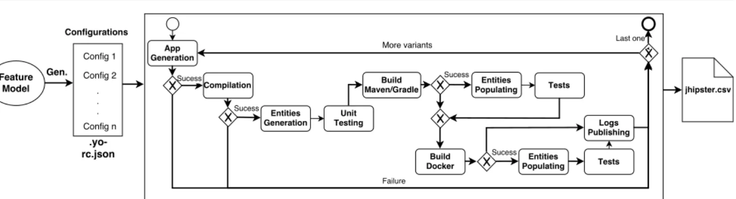
From the feature model, we enumerated all valid con-figurations using solvers and FAMILIAR [4]. We devel-oped a comprehensive workflow for testing each config-uration. Figure 3 summarises the main steps (compila-tion, builds and tests). The first step is to synthesize a .yo-rc.json file from a feature model configuration. It allows us to skip the command-line questions-and-answers-based configurator; the command yo jhipster can directly use such a JSON file for launching the com-pilation of a variant. A monitoring of the whole testing process is performed to detect and log failures that can occur at several steps of the workflow. We faced several difficulties for instrumenting the workflow.
4.2.1 Engineering a configurable system for testing configurations
The execution of a unique and generic command for testing JHipster variants was not directly possible. For instance, the build of a JHipster application relies either on Maven or Gradle, two alternative features of our vari-ability model. We developed varivari-ability-aware scripts to execute commands specific to a JHipster configuration. Command scripts include: starting database services, running database scripts (creation of tables, keyspaces, generation of entities, etc.), launching test commands, starting/stopping Docker, etc. As a concrete example, the inclusion of features h2 and Maven lead to the ex-ecution of the command: “mvnw -Pdev"; the choice of Gradle (instead of Maven) and mysql (instead of h2) in production mode would lead to the execution of an-other command: “gradlew -Pprod". In total, 15 features of the original feature model influence (individually or through interactions with others) the way the testing workflow is executed. The first lessons learned are that (i) a non-trivial engineering effort is needed to build a configuration-aware testing workflow – testing a config-urable system like JHipster requires to develop another configurable system; (ii) the development was iterative and mainly consisted in automating all tasks originally considered as manual (e.g., starting database services).
4.2.2 Implementing testing procedures
After a successful build, we can execute and test a JHip-ster variant. A first challenge is to create the generic
Fig. 3 Testing workflow of JHipster configurations.
Listing 3 JHipster generated JUnit test in
AccountResourceIntTest.java @ T e s t p u b l i c v o i d t e s t A u t h e n t i c a t e d U s e r () ( . . . ) { r e s t U s e r M o c k M v c . p e r f o r m ( get ("/ api / a u t h e n t i c a t e ") . w i t h ( r e q u e s t - > { r e q u e s t . s e t R e m o t e U s e r (" t e s t ") ; r e t u r n r e q u e s t ;}) . a c c e p t ( M e d i a T y p e . A P P L I C A T I O N _ J S O N ) ) . a n d E x p e c t ( s t a t u s () . i s O k () ) . a n d E x p e c t ( c o n t e n t () . s t r i n g (" t e s t ") ) ; }
conditions (i.e., input data) under which all variants will be executed and tested. Technically, we need to populate Web applications with entities (i.e., structured data like tables in an SQL database or documents in MongoDB for instance) to test both the server-side (in charge of accessing and storing data) and the client-side (in charge of presenting data). JHipster entities are cre-ated using a domain-specific language called JDL, close to UML class diagram formalism. We decided to reuse the entity model template given by the JHipster team6. We created 3 entity models for MongoDB, Cassandra, and “others” because some database technologies vary in terms of JDL expressiveness they can support (e.g., you cannot have relationships between entities with a MongoDB database).
After entities creation with JDL (Entities Genera-tion in Figure 3), we run several tests: integraGenera-tion tests written in Java using the Spring Test Context frame-work (see Listing 3 for instance), user interface tests written in JavaScript using the Karma.js framework (see Listing 4 for instance), etc., and create an exe-cutable JHipster variant (Build Maven/Gradle in Fig-ure 3). The tests run at this step are automatically gen-erated and include defaults tests common to all JHip-ster variants and additional tests generated by the JDL entities creation. On average, the Java line coverage is 44.53% and the JavaScript line coverage is 32.19%.
6 https://jhipster.github.io/jdl-studio/
Listing 4 JHipster generated Karma.js test in user.service.spec.ts d e s c r i b e ( ’ C o m p o n e n t Tests ’ , () = > { d e s c r i b e ( ’ L o g i n C o m p o n e n t ’ , () = > { ( . . . ) it ( ’ s h o u l d r e d i r e c t u s e r w h e n r e g i s t e r ’ , () = > { // W H E N c o m p . r e g i s t e r () ; // T H E N e x p e c t ( m o c k A c t i v e M o d a l . d i s m i s s S p y ) . t o H a v e B e e n C a l l e d W i t h ( ’ to s t a t e r e g i s t e r ’) ; e x p e c t ( m o c k R o u t e r . n a v i g a t e S p y ) . t o H a v e B e e n C a l l e d W i t h ([ ’/ r e g i s t e r ’]) ; }) ; ( . . . ) }) ; }) ;
We instantiate the generated entities (Entities Pop-ulating in Figure 3) using the Web user interface through Selenium scripts. We integrate the following testing frame-works to compute additional metrics (Tests in Figure 3): Cucumber, Gatling and Protractor. We also implement generic oracles that analyse and extract log error mes-sages. And finally, repeated two last steps using Docker (Build Docker, Entities Populating, and Tests in Fig-ure 3) before saving the generated log files.
Finding commonalities among the testing procedures participates to the engineering of a configuration-aware testing infrastructure. The major difficulty was to de-velop input data (entities) and test cases (e.g., Selenium scripts) that are generic and can be applied to all JHip-ster variants.
4.2.3 Building an all-inclusive testing environment Each JHipster configuration requires to use specific tools and pre-defined settings. Without them, the compila-tion, build, or execution cannot be performed. A sub-stantial engineering effort was needed to build an in-tegrated environment capable of deriving any JHipster configuration. The concrete result is a Debian image with all tools pre-installed and pre-configured. This pro-cess was based on numerous tries and errors, using
some configurations. In the end, we converged on an all-inclusive environment.
4.2.4 Distributing the tests
The number of JHipster variants led us to consider strategies to scale up the execution of the testing work-flow. We decided to rely on Grid’50007, a large-scale testbed offering a large amount of computational re-sources [10]. We used numerous distributed machines, each in charge of testing a subset of configurations. Small-scale experiments (e.g., on local machines) helped us to manage distribution issues in an incremental way. Distributing the computation further motivated our pre-vious needs of testing automation and pre-set Debian images.
4.2.5 Opportunistic optimizations and sharing
Each JHipster configuration requires to download nu-merous Java and JavaScript dependencies, which con-sumes bandwidth and increases JHipster variant gener-ation time. To optimise this in a distributed setting, we downloaded all possible Maven, npm and Bower depen-dencies – once and for all configurations. We eventually obtained a Maven cache of 481MB and a node_modules (for JavaScript dependencies) of 249MB. Furthermore, we build a Docker variant right after the classical build (see Figure 3) to derive two JHipster variants (with and without Docker) without restarting the whole deriva-tion process.
4.2.6 Validation of the testing infrastructure
A recurring reaction after a failed build was to wonder whether the failure was due to a buggy JHipster vari-ant or an invalid assumption/configuration of our in-frastructure. We extensively tried some selected config-urations for which we know it should work and some for which we know it should not work. Based on some po-tential failures, we reproduced them on a local machine and studied the error messages. We also used statisti-cal methods and GitHub issues to validate some of the failures (see next Section). This co-validation, though difficult, was necessary to gain confidence in our infras-tructure. After numerous tries on our selected config-urations, we launched the testing workflow for all the configurations (selected ones included).
7 https://www.grid5000.fr
4.3 Human Cost
The development of the complete derivation and test-ing infrastructure was achieved in about 4 months by 2 people (i.e., 8 person * month in total). For each activity, we report the duration of the effort realized in the first place. Some modifications were also made in parallel to improve different parts of the solution – we count this duration in subsequent activities.
Modelling configurations. The elaboration of the first major version of the feature model took us about 2 weeks based on the analysis of the JHipster code and configurator.
Configuration-aware testing workflow. Based on the fea-ture model, we initiated the development of the testing workflow. We added features and testing procedures in an incremental way. The effort spanned on a period of 8 weeks.
All-inclusive environment. The building of the Debian image was done in parallel to the testing workflow. It also lasted a period of 8 weeks for identifying all pos-sible tools and settings needed.
Distributing the computation. We decided to deploy on Grid’5000 at the end of November and the implementa-tion has lasted 6 weeks. It includes a learning phase (1 week), the optimization for caching dependencies, and the gathering of results in a central place (a CSV-like table with logs).
(RQ1.1) What is the cost of engineering an infrastructure capable of automatically deriving and testing all configurations? The testing in-frastructure is itself a configurable system and requires a substantial engineering effort (8 man-months) to cover all design, implementation and validation activities, the latter being the most difficult.
4.4 Computational Cost
We used a network of machines that allowed us to test all 26,256 configurations in less than a week. Specifi-cally, we performed a reservation of 80 machines for 4 periods (4 nights) of 13 hours. The analysis of 6 con-figurations took on average about 60 minutes. The total CPU time of the workflow on all the configurations is 4,376 hours. Besides CPU time, the processing of all
variants also required enough free disk space. Each scaf-folded Web application occupies between 400MB and 450MB, thus forming a total of 5.2 terabytes.
We replicated three times our exhaustive analysis (with minor modifications of our testing procedure each time); we found similar numbers for assessing the com-putational cost on Grid’5000. As part of our last ex-periment, we observed suspicious failures for 2,325 con-figurations with the same error message: “Communi-cations link failure”, denoting network communication error (between a node and the controller for instance) on the grid. Those failures have been ignored and con-figurations have been re-run again afterwards to have consistent results.
(RQ1.2) What are the computational resources needed to test all configurations? Testing all con-figurations requires a significant amount of com-putational resources (4,376 hours CPU time and 5.2 terabytes of disk space).
5 Results of the Testing Workflow Execution (RQ2.1)
The execution of the testing workflow yielded a large file comprising numerous results for each configuration. This file8 allows to identify failing configurations, i.e., configurations that do not compile or build. In addition, we also exploited stack traces for grouping together some failures. We present here the ratios of failures and associated faults.
5.1 Bugs: A Quick Inventory
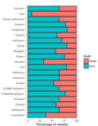
Out of the 26,256 configurations we tested, we found that 9,376 (35.70%) failed. This failure occurred either during the compilation of the variant (Compilation in Figure 3) or during its packaging as an executable Jar file (Build Maven/Gradle in Figure 3, which includes execution of the different Java and JavaScript tests erated by JHipster), although the generation (App gen-eration in Figure 3) was successful. We also found that some features were more concerned by failures as de-picted in Figure 4. Regarding the application type, for instance, microservice gateways and microservice appli-cations are proportionally more impacted than mono-lithic applications or UAA server with, respectively, 58.37% of failures (4,184 failing microservice gateways 8 Complete results are available at https://github.com/
xdevroey/jhipster-dataset/tree/master/v3.6.1. Cassandra DiskBased Docker Ehcache EnableSocialSignIn EnableTranslation Gradle Hazelcast InMemory Jwt Mariadb Maven Mongodb Mysql NoDocker Oauth2 Postgresql Session Spring−websocket Uaa UseSass 0 25 50 75 100 Percentage of variants Build Failed Succ.
Fig. 4 Proportion of build failure by feature
configurations) and 58.3% of failures (532 failing mi-croservice applications configurations). UAA authenti-cation is involved in most of the failures: 91.66% of UAA-based microservices applications (4,114 configu-rations) fail to deploy.
5.2 Statistical Analysis
Previous results do not show the root causes of the configuration failures – what features or interactions between features are involved in the failures? To in-vestigate correlations between features and failures’ re-sults, we decided to use the Association Rule learn-ing method [24]. It aims at extractlearn-ing relations (called rules) between variables of large data-sets. The Asso-ciation Rule method is well suited to find the (combi-nations of) features leading to a failure, out of tested configurations.
Formally and adapting the terminology of associa-tion rules, the problem can be defined as follows.
– let F = {f t1, f t2, . . . , f tn, bs} be a set of n features (f ti) plus the status of the build (bs), i.e., build failed or not;
– let C = {c1, c2, . . . , cm} be a set of m configurations. Each configuration in C has a unique identifier and con-tains a subset of the features in F and the status of its
build. A rule is defined as an implication of the form: X ⇒ Y , where X, Y ⊆ F . The outputs of the method are a set of rules, each constituted by:
– X the left-hand side (LHS) or antecedent of the rule; – Y the right-hand side (RHS) or consequent of the
rule.
For our problem, we consider that Y is a single tar-get: the status of the build. For example, we want to understand what combinations of features lead to a fail-ure, either during the compilation or the build process. To illustrate the method, let us take a small example (see Table 1). The set of features is F = { mariadb, gradle, enableSocialSignIn, websocket, failure } and in the table is shown a small database containing the con-figurations, where, in each entry, the value 1 means the presence of the feature in the corresponding configura-tion, and the value 0 represents the absence of a feature in that configuration. In Figure 1, when build failure has the value 1 (resp. 0), it means the build failed (resp. succeeded). An example rule could be:
{mariadb, graddle} ⇒ {build failure}
Meaning that if mariadb and gradle are activated, con-figurations will not build.
As there are many possible rules, some well-known measures are typically used to select the most interest-ing ones. In particular, we are interested in the support, the proportion of configurations where LHS holds and the confidence, the proportion of configurations where both LHS and RHS hold. In our example and for the rule {mariadb, graddle} ⇒ {build failure}, the support is 2/6 while the confidence is 1.
Table 2 gives some examples of the rules we have been able to extract. We parametrized the method as follows. First, we restrained ourselves to rules where the RHS was a failure: either Build=KO (build failed) or Compile=KO (compilation failed). Second, we fixed the confidence to 1: if a rule has a confidence below 1 then it is not asserted in all configurations where the LHS expression holds – the failure does not occur in all cases. Third, we lowered the support in order to catch all failures, even those afflicting smaller proportion of the configurations. For instance, only 224 configurations fail due to a compilation error; in spite of a low sup-port, we can still extract rules for which the RHS is Compile=KO. We computed redundant rules using fa-cilities of the R package arules.9 As some association rules can contain already known constraints of the fea-ture model, we ignored some of them.
9 https://cran.r-project.org/web/packages/arules/ MoSo Test−Env OASQL MaDo UaEh UaDo MaGr 0 1000 2000 3000 Failures
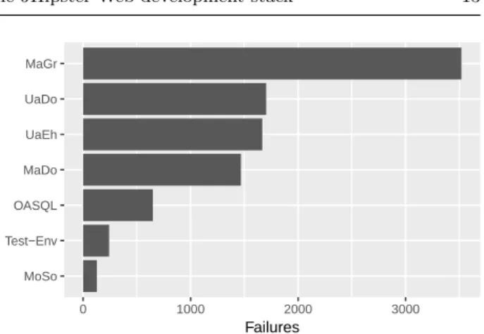
Fig. 5 Proportion of failures by fault described in Table 2.
We first considered association rules for which the size of the LHS is either 1, 2 or 3. We extracted 5 differ-ent rules involving two features (see Table 2). We found no rule involving 1 or 3 features. We decided to examine the 200 association rules for which the LHS is of size 4. We found out a sixth association rule that incidentally corresponds to one of the first failures we encountered in the early stages of this study.
Table 2 shows that there is only one rule with the RHS being Compile=KO. According to this rule, all configurations in which the database is MongoDB and social login feature is enabled (128 configurations) fail to compile. The other 5 rules are related to a build fail-ure. Figure 5 reports on the proportion of failed config-urations that include the LHS of each association rule. Such LHS can be seen as a feature interaction fault that causes failures. For example, the combination of Mari-aDB and Gradle explains 37% of failed configurations (or 13% of all configurations). We conclude that six feature interaction faults explain 99.1% of the failures.
5.3 Qualitative Analysis
We now characterize the 6 important faults, caused by the interactions of several features (between 2 features and 4 features). Table 2 gives the support, confidence for each association rule. We also confirm each fault by giving the GitHub issue and date of fix.
MariaDB with Docker. This fault is the only one caused by the interaction of 4 features: it concerns monolithic web-applications relying on MariaDB as production data-base, where the search-engine (ElasticSearch) is disabled and built with Docker. These variants amount to 1,468 configurations and the root cause of this bug lies in the template file src/main/docker/_app.yml where a con-dition (if prodDB = MariaDB ) is missing.
Table 1 An example of JHipster data (feature values and build status for each configuration). We want to extract association rules stating which combinations of feature values lead to a build failure (e.g., gradle).
Conf. gradle mariadb enableSocialSignIn websocket ... build failure
1 1 0 0 0 ... 0 2 0 1 0 0 ... 0 3 0 0 1 1 ... 0 4 1 1 0 0 ... 1 5 1 0 0 0 ... 0 6 1 1 0 0 ... 1 ... ... ... ... ... ... ...
Table 2 Association rules involving compilation and build failures
Id Left-hand side Right-hand
side
Support Conf. GitHub
Issue
Report/Correction date
MoSo DatabaseType=“mongodb", EnableSocialSignIn=true
Compile=KO 0.488 % 1 4037 27 Aug 2016 (report and
fix for milestone 3.7.0) MaGr prodDatabaseType=“mariadb",
buildTool=“gradle"
Build=KO 16.179 % 1 4222 27 Sep 2016 (report and
fix for milestone 3.9.0)
UaDo Docker=true, authenticationType=“uaa" Build=KO 6.825 % 1 UAA is in Beta Not corrected OASQL authenticationType=“uaa", hibernateCache=“no"
Build=KO 2.438 % 1 4225 28 Sep 2016 (report and
fix for milestone 3.9.0) UaEh authenticationType=“uaa",
hibernateCache=“ehcache"
Build=KO 2.194 % 1 4225 28 Sep 2016 (report and
fix for milestone 3.9.0) MaDo prodDatabaseType=“mariadb",
applicationType=“monolith", searchEngine=“false", Docker=“true"
Build=KO 5.590% 1 4543 24 Nov 2016 (report and
fix for milestone 3.12.0)
MariaDB using Gradle. This second fault concerns vari-ants relying on Gradle as build tool and MariaDB as the database (3,519 configurations). It is caused by a missing dependency in template file server/template/-gradle/_liquibase.gradle.
UAA authentication with Docker. The third fault oc-curs in Microservice Gateways or Microservice applica-tions using an UAA server as authentication mechanism (1,703 Web apps). This bug is encountered at build time, with Docker, and it is due to the absence of UAA server Docker image. It is a known issue, but it has not been corrected yet, UAA servers are still in beta versions.
UAA authentication with Ehcache as Hibernate second level cache. This fourth fault concerns Microservice Gate-ways and Microservice applications, using a UAA authen-tication mechanism. When deploying manually (i.e., with Maven or Gradle), the web application is unable to reach the deployed UAA instance. This bug seems to be re-lated to the selection of Hibernate cache and impacts 1,667 configurations.
OAuth2 authentication with SQL database. This defect is faced 649 times, when trying to deploy a web-app, using an SQL database (MySQL, PostgreSQL or Mari-aDB) and an OAuth2 authentication, with Docker. It
was reported on August 20th, 2016 but the JHipster team was unable to reproduce it on their end.
Social Login with MongoDB. This sixth fault is the only one occurring at compile time. Combining MongoDB and social login leads to 128 configurations that fail. The source of this issue is a missing import in class So-cialUserConnection.java. This import is not in a condi-tional compilation condition in the template file while it should be.
Testing infrastructure. We have not found a common fault for the remaining 242 configurations that fail. We came to this conclusion after a thorough and manual investigation of all logs.10We noticed that, despite our validation effort with the infrastructure (see RQ1), the observed failures are caused by the testing tools and environment. Specifically, the causes of the failures can be categorized in two groups: (i) several network access issues in the grid that can affect the testing workflow at any stage and (ii) several unidentified errors in the configuration of building tools (gulp in our case).
10 Such configurations are tagged by “ISSUE:env” in the
col-umn “bug” of the JHipster results CSV file available online https://github.com/xdevroey/jhipster-dataset.
Feature interaction strength. Our findings show that only two features are involved in five (out of six) faults, and four features are involved in the last fault. The prominence of 2-wise interactions is also found in other studies. Abal et al. report that, for the Linux bugs they have qualitatively examined, more than a half (22/43) are attributed to 2-wise interactions [2]. Yet, for dif-ferent interaction strengths, there is no common trend: we do not have 3-wise interactions while this is second most common case in Linux, we did not find any fault caused by one feature only.
(RQ2.1) How many and what kinds of fail-ures/faults can be found in all configurations? Exhaustive testing shows that almost 36% of the configurations fail. Our analysis identifies 6 in-teraction faults as the root cause for this high percentage.
6 Sampling Techniques Comparison (RQ2.2) In this section, we first discuss the sampling strategy used by the JHipster team. We then use our dataset to make a ground truth comparison of six state-of-the-art sampling techniques.
6.1 JHipster Team Sampling Strategy
The JHipster team uses a sample of 12 representative configurations for the version 3.6.1, to test their gen-erator (see Section 8.1 for further explanations on how these were sampled). During a period of several weeks, the testing configurations have been used at each com-mit (see also Section 8.1). These configurations fail to reveal any problem, i.e., the Web-applications corre-sponding to the configurations successfully compiled, build and run. We assessed these configurations with our own testing infrastructure and came to the same observation. We thus conclude that this sample was not effective to reveal any defect.
6.2 Comparison of Sampling Techniques
As testing all configurations is very costly (see RQ1), sampling techniques remain of interest. We would like to find as many failures and faults as possible with a minimum of configurations in the sampling. For each failure, we associate a fault through the automatic anal-ysis of features involved in the failed configuration (see previous subsections).
We address RQ2.2 with numerous sampling tech-niques considered in the literature [1, 38, 52, 63]. For each technique, we report on the number of failures and faults.
6.2.1 Sampling techniques
t-wise sampling. We selected 4 variations of the t -wise criteria: 1-wise, 2-wise, 3-wise and 4-wise. We gen-erate the samples with SPLCAT [38], which has the advantage of being deterministic: for one given feature model, it will always provide the same sample. The 4 variations yield samples of respectively 8, 41, 126 and 374 configurations. 1-wise only finds 2 faults; 2-wise discovers 5 out of 6 faults; 3-wise and 4-wise find all of them. It has to be noted that the discovery of a 4-wise interaction fault with a 3-wise setting is a ‘collat-eral’ effect [64], since any sample covering completely t-way interactions also yields an incomplete coverage of higher-order interactions.
One-disabled sampling. Using one-disabled sampling algorithm, we extract configurations in which all fea-tures are activated but one. To overcome any bias in selecting the first valid configuration, as suggested by Medeiros et al. [52], we applied a random selection in-stead. We therefore select a valid random configuration for each disabled feature (called one-disabled in our results) and repeat experiments 1,000 times to get sig-nificant results. This gives us a sample of 34 config-urations which detects on average 2.4 faults out of 6.
Additionally, we also retain all-one-disabled con-figurations (i.e., all valid concon-figurations where one fea-ture is disabled and the other are enabled). The all-one-disabled sampling yields a total sample of 922 config-urations that identifies all faults but one.
One-enabled and most-enabled-disabled sampling. In the same way, we implemented sampling algorithms cov-ering the one-enabled and most-enabled-disabled criteria [1, 52]. As for one-disabled, we choose to ran-domly select valid configurations instead of taking the first one returned by the solver. Repeating the experi-ment 1,000 times: one-enabled extracts a sample of 34 configurations which detects 3.15 faults on average; and most-enabled-disabled gives a sample of 2 config-urations that detects 0.67 faults on average. Consid-ering all valid configurations, all-one-enabled extracts a sample of 2,340 configurations and identifies all the 6 faults. All-most-enabled-disabled gives a sample of 574 configurations that identifies 2 faults out of 6.
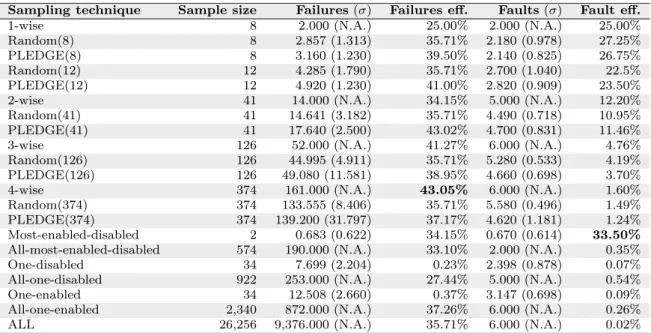
Table 3 Efficiency of different sampling techniques (bold values denote the highest efficiencies)
Sampling technique Sample size Failures (σ) Failures eff. Faults (σ) Fault eff.
1-wise 8 2.000 (N.A.) 25.00% 2.000 (N.A.) 25.00%
Random(8) 8 2.857 (1.313) 35.71% 2.180 (0.978) 27.25%
PLEDGE(8) 8 3.160 (1.230) 39.50% 2.140 (0.825) 26.75%
Random(12) 12 4.285 (1.790) 35.71% 2.700 (1.040) 22.5%
PLEDGE(12) 12 4.920 (1.230) 41.00% 2.820 (0.909) 23.50%
2-wise 41 14.000 (N.A.) 34.15% 5.000 (N.A.) 12.20%
Random(41) 41 14.641 (3.182) 35.71% 4.490 (0.718) 10.95%
PLEDGE(41) 41 17.640 (2.500) 43.02% 4.700 (0.831) 11.46%
3-wise 126 52.000 (N.A.) 41.27% 6.000 (N.A.) 4.76%
Random(126) 126 44.995 (4.911) 35.71% 5.280 (0.533) 4.19%
PLEDGE(126) 126 49.080 (11.581) 38.95% 4.660 (0.698) 3.70%
4-wise 374 161.000 (N.A.) 43.05% 6.000 (N.A.) 1.60%
Random(374) 374 133.555 (8.406) 35.71% 5.580 (0.496) 1.49%
PLEDGE(374) 374 139.200 (31.797) 37.17% 4.620 (1.181) 1.24%
Most-enabled-disabled 2 0.683 (0.622) 34.15% 0.670 (0.614) 33.50%
All-most-enabled-disabled 574 190.000 (N.A.) 33.10% 2.000 (N.A.) 0.35%
One-disabled 34 7.699 (2.204) 0.23% 2.398 (0.878) 0.07%
All-one-disabled 922 253.000 (N.A.) 27.44% 5.000 (N.A.) 0.54%
One-enabled 34 12.508 (2.660) 0.37% 3.147 (0.698) 0.09%
All-one-enabled 2,340 872.000 (N.A.) 37.26% 6.000 (N.A.) 0.26%
ALL 26,256 9,376.000 (N.A.) 35.71% 6.000 (N.A.) 0.02%
Dissimilarity sampling. We also considered dissimilar-ity testing for software product lines [5,27] using PLE-DGE [30]. We retained this technique because it can afford any testing budget (sample size and generation time). For each sample size, we report the average fail-ures and faults for 100 PLEDGE executions with the greedy method in 60 secs [30]. We selected (respec-tively) 8, 12, 41, 126 and 374 configurations, finding (respectively) 2.14, 2.82, 4.70, 4.66 and 4.60 faults out of 6.
Random sampling. Finally, we considered random sam-ples from size 1 to 2,500. The random samsam-ples exhibit, by construction, 35.71% of failures on average (the same percentage that is in the whole dataset). To compute the number of unique faults, we simulated 100 random selections. We find, on average, respectively 2.18, 2.7, 4.49, 5.28 and 5.58 faults for respectively 8, 12, 41, 126 and 374 configurations.
6.2.2 Fault and failure efficiency
We consider two main metrics to compare the efficiency of sampling techniques to find faults and failures w.r.t the sample size. Failure efficiency is the ratio of failures to sample size. Fault efficiency is the ratio of faults to sample size. For both metrics, a high efficiency is desir-able since it denotes a small sample with either a high failure or fault detection capability.
The results are summarized in Table 3. We present in Figure 6(a) (respectively, Figure 6(b)) the evolution of failures (respectively, faults) w.r.t. the size of random
samples. To ease comparison, we place reference points corresponding to results of other sampling techniques. A first observation is that random is a strong baseline for both failures and faults. 2-wise or 3-wise sampling techniques are slightly more efficient to identify faults than random. On the contrary, all-enabled, one-enabled, all-one-disabled, one-disabled and all-most-enabled-disabled identify less faults than random sam-ples of the same size. Most-enabled-disabled is efficient on average to detect faults (33.5% on average) but re-quires to be “lucky". In particular, the first configura-tions returned by the solver (as done in [52]) discovered 0 fault. This shows the sensitivity of the selection strat-egy amongst valid configurations matching the most-enabled-disabled criterion. Based on our experience, we recommend researchers the use of a random strategy in-stead of picking the first configurations when assessing one-disabled, one-enabled, and most-enabled-disabled.
PLEDGE is superior to random for small sample sizes. The significant difference between 2-wise and 3-wise is explained by the sample size: although the latter finds all the bugs (one more than 2-wise) its sample size is triple (126 configurations against 41 for 2-wise). In general, a relatively small sample is sufficient to quickly identify the 5 or 6 most important faults – there is no need to cover the whole configuration space.
A second observation is that there is no correlation between failure efficiency and fault efficiency. For ex-ample, all-one-enabled has a failure efficiency of 37.26% (better than random and many techniques) but is one of the worst techniques in terms of fault rate due of its high sample size. In addition, some techniques, like
all-● ● ● ● ● ● 0 250 500 750 0 500 1000 1500 2000 2500 Configurations F ailures f ound Sampling ● ● ● ● ● ● 1−wise 2−wise 3−wise 4−wise All−most−en.−dis. All−one−dis. All−one−en. Most−en.−dis. One−dis. One−en. PLEDGE(12) PLEDGE(126) PLEDGE(374) PLEDGE(41) PLEDGE(8) Random
(a) Failures found by sampling techniques
● ● ● ● ● ● 2 4 6 0 500 1000 1500 2000 2500 Configurations F aults f ound Sampling ● ● ● ● ● ● 1−wise 2−wise 3−wise 4−wise All−most−en.−dis. All−one−dis. All−one−en. Most−en.−dis. One−dis. One−en. PLEDGE(12) PLEDGE(126) PLEDGE(374) PLEDGE(41) PLEDGE(8) Random
(b) Faults found by sampling techniques Fig. 6 Defects found by sampling techniques
most-enable-disabled, can find numerous failures that in fact correspond to the same fault.
6.2.3 Discussion
Our results show that the choice of a metric (failure-detection or fault-(failure-detection capability) can largely in-fluence the choice of a sampling technique. Our initial assumption was that the detection of one failure leads to the finding of the associated fault. The GitHub reports and our qualitative analysis show that it is indeed the case in JHipster: contributors can easily find the root causes based on a manual analysis of a configuration failure. For other cases, finding the faulty features or feature interactions can be much more tricky. In such contexts, investigating many failures and using statis-tical methods (such as association rules) can be helpful to determine the faulty features and their undesired in-teractions. As a result, the ability of finding failures may be more important than in JHipster case. A trade-off between failure and fault efficiency can certainly be considered when choosing the sampling technique.
(RQ2.2) How effective are sampling techniques comparatively? To summarise: (i) random is a strong baseline for failures and faults; (ii) 2-wise and 3-wise sampling are slightly more efficient to find faults than random; (iii) most-enabled-disabled is efficient on average to detect faults but requires to be lucky; (iv) dissimilarity is su-perior to random for small sample sizes; (v) a small sample is sufficient to identify most impor-tant faults, there is no need to cover the whole configuration space; and (vi) there is no corre-lation between failure and fault efficiencies.
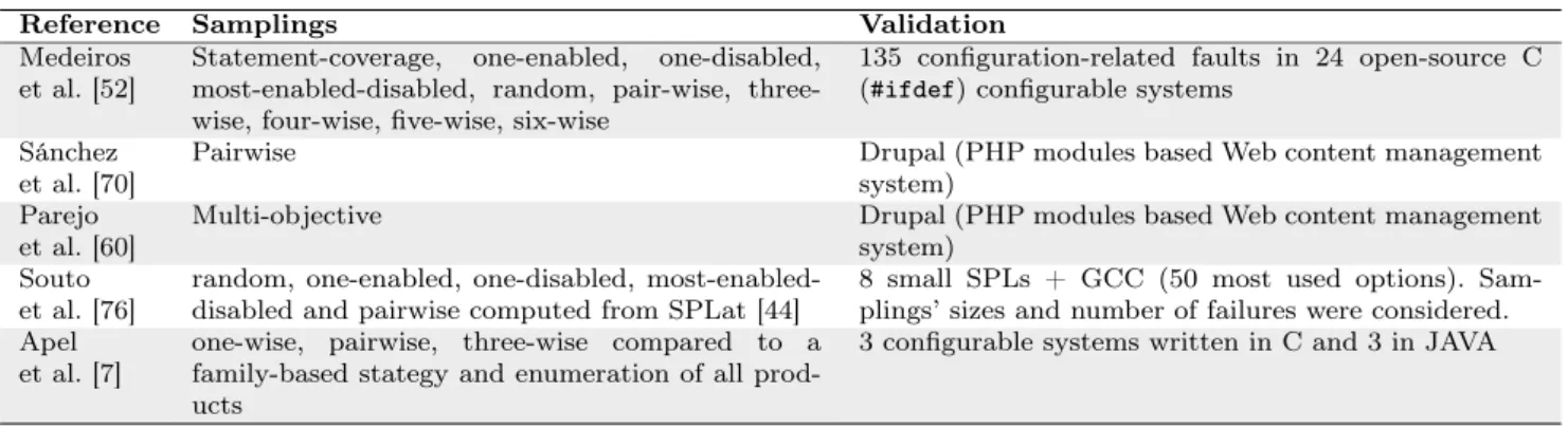
7 Comparison with Other Studies (RQ2.3) This section presents a literature review of case stud-ies of configuration sampling approaches to test vari-ability intensive systems. Specifically, we aim to com-pare our findings with state-of-the-art results: Are sam-pling techniques as effective in other case studies? Do our results confirm or contradict findings in other set-tings? This question is important for (1) practitioners in charge of establishing a suitable strategy for test-ing their systems; (ii) researchers interested in buildtest-ing evidence-based theories or tools for testing configurable systems.
We first present our selection protocol of relevant papers and an overview of the selected ones. We then confront and discuss our findings from Section 6.2 w.r.t. those studies.