Propagation modeling using Split Step Fourier Method: Ground boundary condition analysis and acceleration by GPU

HAL Id: hal-01083706

https://hal.archives-ouvertes.fr/hal-01083706

Submitted on 21 Nov 2014

HAL is a multi-disciplinary open access

archive for the deposit and dissemination of

sci-entific research documents, whether they are

pub-lished or not. The documents may come from

teaching and research institutions in France or

abroad, or from public or private research centers.

L’archive ouverte pluridisciplinaire HAL, est

destinée au dépôt et à la diffusion de documents

scientifiques de niveau recherche, publiés ou non,

émanant des établissements d’enseignement et de

recherche français ou étrangers, des laboratoires

publics ou privés.

Propagation modeling using Split Step Fourier Method:

Ground boundary condition analysis and acceleration by

GPU

V. Fabbro, M. Noblet, R. Lahaye, N. Pinel, C. Bourlier

To cite this version:

V. Fabbro, M. Noblet, R. Lahaye, N. Pinel, C. Bourlier. Propagation modeling using Split Step

Fourier Method: Ground boundary condition analysis and acceleration by GPU. Radar 2014, Oct

2014, LILLE, France. �hal-01083706�

Propagation modeling using Split Step Fourier

Method: Ground boundary condition analysis and

acceleration by GPU

Fabbro Vincent

DEMR/RCP ONERA Toulouse, France vincent.fabbro@onera.fr

Noblet Mathieu, Lahaye Robert, Pinel Nicolas

Alyotech

Rennes, France mathieu.noblet@alyotech.fr

robert.lahaye@alyotech.fr

Bourlier Christophe IETR, LUNAM University

Polytech Nantes Nantes, France

Christophe.bourlier@univ-nantes.fr

Abstract— Forward propagation above dielectric surface is

studied using Split Step Fourier resolution technique (SSF). Introduction of Fresnel Boundary Conditions (SSF-FBC) and Leontovitch Boundary Conditions (SSF-LBC) are described. The numerical singularity induced by reflection coefficient at pseudo Brewster incidence is analyzed and the DMFT solution for SSF-LBC resolution is retrieved. The limit induced by Leontovitch assumption is studied on typical grounds. Numerical validations of the proposed method are presented by comparison to asymptotic formulation. As SSF is based on FFT algorithm, acceleration using GPU implementation is studied and numerical time gain are given.

Keywords— Parabolic Wave Equation, Split Step Fourier, Forward Propagation, Leontovitch Boundary Condition, Fresnel coefficient, GPU acceleration

I. INTRODUCTION

TO model electromagnetic system range at long distances in low troposphere, the Parabolic Wave Equation method (PWE) is usually used. It allows to take into account large-scale refraction effects inducing ducting effect [1][2], small-scale refraction effects inducing scintillation [3][4], and relief effects inducing multipath and masking [5][6]. The propagation of ground wave at HF and lower band can also be modeled [7][8]. To solve PWE, the Split-Step Fourier method (SSF) is the most efficient technique because it uses Fast Fourier Transform (FFT) and permits large step in range. In PWE resolution, classically, boundary conditions at the ground limit is introduced via the Leontovitch impedance boundary condition [9]. The Discrete Mixed Fourier Transform method (DMFT) proposed by Dockery and Kuttler [10] is nowadays currently used in operational system modeling tools [11][26].

This work was supported in part by the French ministry of the “Redressement Productif (Direction Générale de la Compétitivité, de l’Industrie et des Services)”, in the framework of the PRORASEM project, in cooperation between ONERA, ALYOTECH and UNAN-IETR.

However, to model the dielectric interface effect in SSF resolution, the most rigorous method consists in introducing Fresnel reflection coefficient in the spectral domain. Several authors have proposed such an approach as Janaswamy [12]. A similar method has been proposed for SSF technique applied in acoustics domain by Gilbert and Di [13]. More recently, Chabory et al. [14] proposed a formulation based on this idea for the forward propagation computation, for a domain of finite height. However, a numerical problem occurs in the application of this formulation near the Brewster (or pseudo-Brewster) incidences. A first solution has been proposed by Sprouse and Awadallah [15] through the IBC method (Impedance Boundary Condition).

The spectral introduction of reflection coefficient is here revisited considering the boundary condition proposed by Leontovitch (SSF-LBC) or the Fresnel coefficients SSF-FBC at the boundary. The discontinuity induced by the reflection coefficient is illustrated. The relation between SSF-LBC and DMFT is demonstrated, and it shows that the discontinuity is avoided. As the Leontovitch boundary condition is assumed, its limits are studied. In a last section, acceleration of Fourier transform using GPU implementation is illustrated.

II. SSF RESOLUTION OF PWE

The problem of radio-wave propagation above terrestrial surface is reduced to a 2D scalar problem in a vertical plane including the transmitter and the observation point. The problem is solved considering only the transversal component of the field, using the variable change [1]:

( )

_{( ) ( )}

_{( )}

( )

( )

( )

( )

( )

     ≈ = ≈ = + x k r H r H z x m a x a k e u pol V x k r E r E a x a k e u pol H a z a z 0 0 2 / 0 0 2 / , / sin : / sin : φ φ φ φ (1)

where a is the earth radius (approximately 6370 km), x the curvilinear distance at the earth surface, z the altitude (considered small with regard to earth radius), E_φ or Hφ the

transversal component to the vertical propagation plane of the electric or magnetic field and m the modified refraction index. This way, the propagation equation is the 2D Helmholtz equation: , 0 2 2 0 2 2 2 2 =       + ∂ ∂ + ∂ ∂ u m k z x (2) where ko is the wave number in vacuum. The propagation is

modeled along horizontal axis x and z is the vertical axis. The operator

_{( )}

z x m k z Q 2 02 2 , 2 + ∂ ∂

= can be introduced. Reminding the

modified index definition m=M.10−6+1 _{where M is the}

refractivity, and that m is with close to 1 in the atmosphere, a Taylor series expansion is applied:

(

1 2 .10 6

)

.

2 _{≈ + M} −

m (3)

From this approximation, Q can be written following Feit and Fleck formulation [16]:

( )

, .106. 0 2 0 2 2 − + + ∂ ∂ = k kM xz z Q . (4) This approximation is named Wide Angle approximation because it makes appear the exact spectral propagation term in free space under the square root. The solution corresponding to forward propagation is obtained, in the form:

(

x x z

)

e u

( )

x z

u +

δ

, = jQδx , _. (5)

Being aware that the refractivity varies slowly with range, it is assumed to neglect its variations between each step in range along x. Then, the solution can be reformulated:

(

)

( )

_{( )}

_, 10 . , , 2 0 2 2 6 0      + ∂ ∂ = = = + − + k z B M k A with z x u e z x x u δ jδxA B (6) and

(

x x,z

)

e u

( )

x,z u A B A x j       + + δ = δ + 2 2 . (7) This scheme induces a third order error in δx [1]. This equation is solved iteratively in range, applying direct and inverse Fourier transform along the vertical direction, to get the SSF resolution:

(

)

( )

∫

∫

∞ + ∞ − −         ∞ + ∞ − +         − − × = + ' ' , 2 , ' 2 10 . 2 10 . 6 6 0 dz e z x u e e e dk e z x x u z jk M x jk z jk x jk z M x jk z x z x δ δ δ π δ (8) 2 2 0 2 with kx =k −kz.

III. RESOLUTION WITH GROUND BOUNDARY CONDITIONS

In this paper, to simplify the formulations and focus on boundary conditions, the free space atmosphere (M=0) is assumed. Ground can be introduced following the formulation derived by Janaswamy [12] or Gilbert and Di [13]:

(

)

[

(

) ( ) (

)

]

s z z z z z jk x jk u dk k x u k k x u e e z x x u + =

∫

x z +Γ − + +∞ ∞ − + π δ δ 2 , ~ , ~ , (9)

where the reflection coefficient is in the spectral domain is

( )

g z g z z k k k k k + − = Γ . (10) and s

u is the Zenneck surface wave that can be neglected for

microwave applications. For the Fresnel reflection coefficient:

π µ σλ ε 2 ; 2 0 2 2 2 2 0 2 2 2 0 c j n n k n k k k n k k r x gV x gH + = − = − = (11)

where εr and σ are the ground relative permittivity and

conductivity respectively, λ the wavelength and c the light speed (H and V stands for polarization). The field continuity at the interface is insured by applying the reflection Fresnel coefficient above the ground and the transmission Fresnel coefficient in the ground. This resolution is called SSF-FBC. For SSF-LBC resolution, the Leontovitch hypothesis is assumed [9], and kg becomes:

(

)

(

)

2 2 2 0 / 2 2 0 1 1 n n k k n k k gV gH − ≈ − ≈ (12)

The complete reduced field satisfies the Leontovitch boundary condition [9] on the ground, leading to:

(

=0

)

=0. + ∂ ∂ = z u jk z u g O z (13)

IV. NUMERICAL PROBLEM AT PSEUDO BREWSTER ANGLE

For SSF-FBC and SSF-LBC, the numerical computation of the integral in (9) containing the reflection coefficient can induce a numerical problem for some types of ground. Sprouse [15] also studied this problem, related to the Brewster angle

B

θ (or called the pseudo-Brewster angle for a ground with losses) for which the reflection coefficient amplitude is very small. Reminding the property of the spectral reflection coefficient:

( ) ( )

θ =Γ−θ Γ 1 , (14) when kz tends to B B z k

k =− ₀sin

θ

the reflection coefficient tends to infinity. As an illustration, in Fig.1 is represented the variations of spectral Fresnel reflection coefficient versus grazing angle from negative to positive values. This integration domain is imposed by the definition of the Fourier transform. Different typical soils have been considered: sea, wet ground, medium dry ground and very dry ground. The dielectric constants have been estimated from the values proposed by the International Telecommunication Union [20]. At pseudo Brewster angle, the amplitude of reflection coefficient can be very close to zero and a sign change of its

real part appears when this angle is passed, involving a phase sign variation. In parallel, a very big value of the reflection coefficient modulus is involved at _−θB of the pseudo Brewster angle, in negative k_z domain, for wet ground, medium dry ground and very dry ground. In fig. 1 is also represented the spectral reflection coefficients assuming the Leontovitch approximation. Compared to the Fresnel reflection coefficient, the Leontovitch one is very close except for very dry ground for which a grazing angle shift appears, this phenomenon can be observed clearly for negative values of

θ

.

Fig. 1. Comparison of Fresnel and Leontovitch spectral reflection coefficients, V polarization, 1 GHz, for sea, wet ground, medium dry ground and very dry ground.

Sprouse et al. [13] proposed a solution to this problem based on a decomposition of the reduced field u into an odd and even solution, driven by an empirical coefficient δ. Another approach is proposed here, based on SSF-LBC resolution. The discontinuity appears when the reflection coefficient is introduced in the complete reduced spectrum:

(

)

(

)

(

)

        −         + − + = + + z g z g z z x jk z u x k k k k k k x u e k x x u~ δ _, xδ ~ _, ~ _, . (15)

To avoid the numerical problem, the denominator of the reflection coefficient is multiplied to the solution and a new variable w~

(

x+δx,k_z

)

defined:

(

,

)

[

~

(

,

)

(

) (

)

~

(

,

)

]

. ~ z g z g z z x jk z e u x k k k k k u x k k x x w +δ = + xδ + + − − . (16) Then, the problem is solved from this new variable w propagated in range. After Fourier transform, in spatial domain one obtains:

(

)

+∞

∫

(

)

(

)

∞ − + _{+ +} = + . 2 , ~ , π δ δ z g z z z jk dk k k k x x u e z x x w z . (17)

Considering the Fourier transform properties, one can note that u

(

x+

δ

x,z

)

and w

(

x+

δ

x,z

)

are related in spatial domain by

(

,

)

(

,

)

k u

(

x x,z

)

. dz z x x du j z x x w g δ δ δ =− + + + + (18)

Thus, w

(

x+δx,z

)

=0 at the interface imposes Leontovitch boundary condition (13) and the proposed variable change is identical to the one proposed in DMFT approach [10]. The difference is the introduction of the ground impedance in spectral domain of k_z variables instead of spatial domain z. From this form, the DMFT can be recovered, starting from (17) and introducing (15). Then it comes:

(

)

[

(

)

(

)

(

)

(

)

]

_π δ δ 2 , ~ , ~ , z z g z g z z x jk z jk dk k x u k k k k k x u e e z x x w z x − − + + = + +∞

_∫

∞ − + + (19)

and this equation can be written

(

)

(

)

(

)

(

)

∫

∞ + ∞ − + − + _{− +} = + . 2 , ~ , π δ δx z jk g z z z jk z jk dk e k k k x u e e z x x w x z z (20)

This formulation makes appear a sine transform, equivalent to DMFT formulation. This way is demonstrated that DMFT resolution implicitly considers the spectral variations of the reflection coefficient, under the approximation of Leontovitch. But, Sprouse and Awadallah [15] shown that DMFT did model well the reflection at V polarization and at the Brewster incidence. This demonstration suggests that it should not be a problem of boundary condition formulation, but a numerical problem. Efficient solutions computing w(x,z) in spatial domain as for the DMFT backward resolution, or using exponential Euler resolution [21] give good results.

To validate this resolution of SSF-LBC, a propagation computation at 1 GHz is proposed, compared to the asymptotic solution considering the image principle applied to an ideal spherical wave in free space and its image weighted by the Fresnel reflection coefficient. This classical solution is described in [12] or [22].

Fig. 2. Propagation factor (dB) vs altitude, at 1 GHz, V pol., distance 5km, computed by asymptotic and SSF-LBC methods above (a) sea surface, (b) wet ground.

Smooth ground, V polarization, the isotropic source at 10 meters above ground, and the results are represented with regard to the altitude at a distance of 5 km. 4 graphs are reported corresponding to different realistic ground: Fig.2.a sea surface, Fig.2.b wet ground, Fig.3.a medium dry ground and Fig.3.b very dry ground. A very good agreement can be noticed. These results demonstrate the availability of the SSF-LBC to model pseudo-Brewster reflection, avoiding the numerical problem.

Fig. 3. Propagation factor (dB) vs altitude, at 1 GHz, V pol., distance 5 km, computed by asymptotic and SSF-LBC methods above (a) medium dry ground, (b) very dry ground.

Unfortunately, the solution proposed for SSF-LBC method is very difficult to apply to the SSF-FBC method. Then, the limits induced by Leontovitch boundary condition compared to rigorous Fresnel boundary condition limit are studied in the next section.

V. STUDY OF LEONTOVITCH BOUNDARY LIMIT

The results obtained at pseudo-Brewster incidence above smooth surface tend to demonstrate that the Leontovith boundary condition gives results quasi identical to the approach using Fresnel reflection coefficient. However, if a zoom is applied to Fig 3.b around the pseudo Brewster incidence (30°) for very dry gound at 1 GHz, a shift appears between asymptotic and SSF-LBC results. This zoom is reported in Fig. 4. The pseudo-Brewster incidence is slightly different with the Leontovitch boundary condition, appearing at 28.1° instead of 30°. The dynamics of the propagation factor, resulting of the combination of the direct and reflected components, is also affected around the precise pseudo-Brewster angle: the interference figure is slitly shifted. To analyze carefully the limit induced by Leontovitch boundary condition, the Fresnel and Leontovith reflection coefficients have been compared for the chosen typical surfaces with a large variation in frequency. To characterize the ground dielectric constants for each frequency, the values proposed by ITU [20] have been used. At V polarization, the minimum of the reflection coefficient modulus

θ

_Bis researched, applying:

( )

at B d d θ θ θ θ Γ =0 = 2 (21)

where

θ

_B is the pseudo Brewster angle.

Fig. 4. Zoom of Propagation factor (dB) vs altitude, around pseudo-Brewster incidence, at 1 GHz, V pol., distance 5 km, computed by asymptotic and PWE-LBC methods above very dry ground.

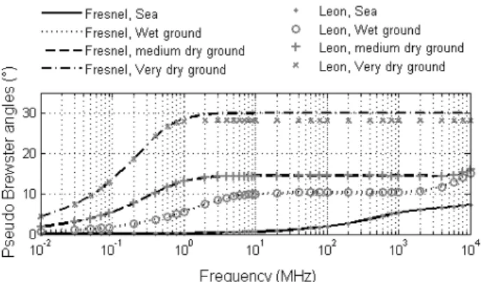
The obtained pseudo-Brewster angles are plotted versus frequency for each material in fig 5. Fresnel and Leontovitch reflection coefficients induce very close pseudo-Brewster angles at all frequencies, except for very dry ground condition.

Fig. 5. For sea, wet ground, medium dry ground, very dry ground: variations of pseudo-Brewster angle with frequency modeled by Fresnel and Leontovith reflection coefficient.

The material very dry ground is the one presenting the lowest values of relative permittivity and conductivity. It is the only one, among the chosen materials, inducing an error on pseudo-Brewster angle estimation by the Leontovitch approximation with a maximum value of around 2° beyond 1 MHz. The error is negligible for lower frequencies. Globally, it appears that Leontovitch remains a good approximation for natural material but materials with low dielectric constant must be considered carefully.

VI. SSF ACCELERATION BY GPU IMPLEMENTATION

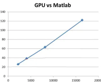
For operational applications, the better time performances of propagation computation are researched. PWE method applied at high frequency, high altitude domain and large beamwidth antennas should induce high computation time. To improve the computation, a hybrid method has been proposed using XO (eXtended Optics) method to extend PWE solution at high altitudes [24]. The last is faster than PWE alone but not perfectly rigourous, particularly above relief. Using fast resolution of Discrete Fourier Transform, the SSF algorithm can be applied to the complete domain without loss of accuracy. In fig. 6 an example of time gain obtained between GPU and Matlab implementations of the same algorithm using SSF resolution is presented. This result has been obtained for a domain of 2 km of altitude, a distance of 100 km and frequencies between 100 MHz and 10 GHz. The Time gain is here plotted with regard to the number of points used for Fast Fourier Transform computation. The gain is significant and grows with the number of points. This type of implemantation appears very efficient for the problem of SSF resolution.

Fig. 6. Time Gain between GPU and Matlab implementation of SSF.

VII. CONCLUSION

First, boundary conditions for ground introduction in SSF algorithm have been studied. The singularity induced by the reflection coefficient introduction in spectral domain is specifically studied. A solution is proposed for SSF-LBC resolution and its relation to the classical DMFT method is given. The limits of Leontovitch boundary condition are then studied on realistic surfaces and at pseudo Brewster angle. The results demonstrate that, for realistic ground characteristics, Leontovitch approximation remains a very good approximation even at V polarization and pseudo Brewster angle. The proposed SSF method can be used to model forward propagation taking into account ducting, above rough sea surfaces or reliefs using linear shift map [6] or stair-case method [24], and considering surface wave propagation at low frequency band. Using GPU implementation, the time gain is

significant and such a tool is adapted for operational applications.

REFERENCES

[1] M. Levy, Parabolic equation methods for electromagnetic wave

propagation. IEE electromagnetic series 45, 2000.

[2] J. R. Kuttler, G. D. Dockery "Theoretical description of the parabolic approximation/Fourier split-step method of representing electromagnetic propagation in the troposphere," Radio Sci., vol. 26, no. 2, pp. 381-393, 1991.

[3] D. Rouseff, "Simulated Microwave Propagation through Tropospheric Turbulence," IEEE Trans. Antennas Propagat., vol. 40, no. 9, pp. 1076-1083, 1992.

[4] V. Fabbro, L. Féral, “Comparison of 2D and 3D electromagnetic approaches to predict tropospheric turbulence effects in clear sky conditions,” IEEE Trans. Antennas Propagat., vol. 60, no. 9, pp. 4398– 4407, sept. 2012.

[5] A. E. Barrios, “Parabolic equation modeling in horizontally inhomogeneous environments,” IEEE Trans. Antennas Propagat., vol. 40, pp. 791–797, 1992.

[6] D. J. Donohue, and J. R. Kuttler, “Propagation modeling over terrain using the parabolic wave equation,” IEEE Trans. Antennas Propagat., vol. 48, no. 2, pp. 260–277, 2000.

[7] G. Apaydin, L. Sevgi, "A Novel Split-Step Parabolic-Equation Package for Surface-Wave Propagation Prediction Along Multiple Mixed Irregular-Terrain Paths," IEEE Antennas Propagat. Mag. Vol. 52, no. 4, pp. 90 - 97, 2010.

[8] V. Fabbro, P. F. Combes, N. Guillet, “Apparent radar cross section of a large target illuminated by a surface wave above the sea,” Progress In

Electromagnetics Research, PIER 50, pp. 41–60, 2005.

[9] M. A. Leontovitch, “On the approximate boundary conditions for an Electromagnetic Field on the surface of well-conducting bodies,” in

Investigations of propagation of radio Waves, in B.A. Vedensky ed.,

Academy of science of USSR, Moscow, 1948.

[10] G. D. Dockery, J.R. Kuttler "An Improved Impedance Boundary Algorithm for Fourier Split-Step Solutions of the Parabolic Wave Equation," IEEE Trans. Antennas Propagat., vol. 44, no. 12, pp. 1592 - 1599, Dec. 1996.

[11] E. Brookner, P. R. Cornely, ; Y.F. Lok,”AREPS and TEMPER, Getting Familiar with these Powerful Propagation Software Tools,” pages 1034 – 1043, Radar Conference 2007.

[12] R. Janaswamy, “Radio wave propagation over a nonconstant immittance plane,” Radio Sci., vol. 36, vol. 3, pp. 387–405, Jan. 2001.

[13] K. E. Gilbert, Xiao Di, “A fast Green's function method for one-way sound propagation in the atmosphere,” J. Acoust. Soc. Am. 94 (4), 1993. [14] A. Chabory, C.Morlass R. Douvenot, B. Souny, “An exact

representation of the wave equation for propagation over terrain,”

Electromagnetics in Advanced Applications (ICEAA), 2012.

[15] C. R. Sprouse, R. S. Awadallah, “An Angle-Dependent Impedance Boundary Condition for the Split-Step Parabolic Equation Method,”

IEEE Trans. Antennas Propagat., vol. 60 , no. 2 , Part: 2, pp. 964 – 970,

Feb. 2012.

[16] M. D. Feit, J. A. Fleck, "Light propagation in grad-index fibers," Appl.

Opt., vol. 17, 3990-3998, 1978.

[17] J. Zenneck, "Propagation of Plane EM Waves Along a Plane Conducting Surface," Ann. Phys. (Leipzig), 23, pp. 846-866, 1907.

[18] K. E. Gilbert and Xiao Di, “An exact point source starting field for the Fourier parabolic equation in outdoor sound propagation,” JASA Express

letters (online version) :12 April 2007, Print version: J. Acoust. Soc. Am.

121 (5), May 2007.

[19] J. R. Kuttler, R. Janaswamy, "Improved Fourier Transform for solving the parabolic wave equation,” Radio Sci., vol.37, no. 2, 2002.

[20] ITU Recommendation P527-3, Electrical characteristics of the surface of the Earth, ITU, 1992.

[21] B. V. Minchev, “Exponential Integrators for Semilinear Problems,” PhD, University of Bergen, August 2004.

[22] V. Fabbro, C. Bourlier , P. F. Combes “Forward propagation modeling above gaussian rough surfaces by the Parabolic wave equation: introduction of the shadowing effect,” Progress In Electromagnetics

[23] W. Ament, “Toward a theory of reflection by a rough surface,” IRE

Proc., vol. 41, pp. 142–146, 1953.

[24] A. E. Barrios, “A terrain parabolic equation model for propagation in the troposphere,” IEEE Trans. Antennas Propag., vol. 42, no. 1, pp. 90 - 98, Jan. 1994.

[25] H. Hitney, “Hybrid ray optics and Parabolic Equation for radar propagation modeling”, radar 92, Brighton, pp. 58 – 61, 12-13 Oct 1992.

[26] J. Claverie, E. Mandine, Y. Hurtaud, “Simulation of radar performances, PREDEM a new tool for the french Navy”, BACIMO, Monterey USA, 2005.