A Statistical Approach to Topological Data Analysis

(1)

HAL Id: tel-01235080

https://tel.archives-ouvertes.fr/tel-01235080

Submitted on 27 Nov 2015

HAL is a multi-disciplinary open access

archive for the deposit and dissemination of sci-entific research documents, whether they are pub-lished or not. The documents may come from teaching and research institutions in France or abroad, or from public or private research centers.

L’archive ouverte pluridisciplinaire HAL, est destinée au dépôt et à la diffusion de documents scientifiques de niveau recherche, publiés ou non, émanant des établissements d’enseignement et de recherche français ou étrangers, des laboratoires publics ou privés.

A Statistical Approach to Topological Data Analysis

Bertrand Michel

To cite this version:

Bertrand Michel. A Statistical Approach to Topological Data Analysis. Statistics [math.ST]. UPMC Université Paris VI, 2015. �tel-01235080�

(2)

MÉMOIRE D’HABILITATION À DIRIGER DES RECHERCHES

Université Pierre et Marie Curie

Laboratoire de Statistique Théorique et Appliquée

Bertrand MICHEL

A Statistical Approach to Topological

Data Analysis

soutenue le 24 novembre 2015

devant le jury composé de :

M. Gérard Biau Université Pierre et Marie Curie Examinateur

M. Benoît Cadre ENS Rennes Rapporteur

M. Frédéric Chazal INRIA Saclay Examinateur

M. Albert Cohen Université Pierre et Marie Curie Président du jury M. Wolfgang Polonik University of California at Davis Rapporteur

M. Pascal Massart Université Paris Sud Examinateur

et au vu du rapport également écrit par :

(3)

(4)

Remerciements

Je souhaite tout d’abord remercier ici chaleureusement Benoît Cadre, Wolfgang Polonik et Shmuel Weinberger d’avoir accepté de rapporter mon mémoire d’habilitation. Wolfgang, I am very honored that you have accepted to review my habilitation thesis and that you came from Davis for my defense. Shmuel, I am also very honored that you have accepted to review my statistical works about topological data analysis.

Le travail présenté dans ce mémoire est le fruit de collaborations et d’interactions avec de nom-breuses personnes que je souhaite vivement remercier.

Je souhaite en premier lieu remercier Pascal Massart et Thomas Duquesne pour m’avoir initié pendant ma thèse au métier d’enseignant-chercheur. Pascal, le soutien que tu as apporté par la suite à ce "mariage" de la statistique et de l’inférence géométrique a été très important pour moi. Thomas, un jour peut-être publierons-nous ce vieux papier qui traîne dans nos placards, mais ce n’est pas le bon moment, le baril est au plus bas.

Je tiens ensuite à remercier très vivement Frédéric Chazal, qui en dépit de mon passé peu recom-mandable de "statisticien pétrolier", m’a accueilli en post-doc à l’INRIA dans l’équipe Geometrica pour travailler sur ces problématiques mêlant statistique, géométrie algorithmique et analyse des données. Frédéric, je suis très heureux de collaborer avec toi sur ces jolies questions. Je te remercie aussi pour la place que tu m’as faite au sein de l’équipe et j’espère que je pourrai continuer à participer activement aux activités de l’équipe DataShape qui devrait prochainement remplacer Geometrica.

J’ai eu la chance de co-encadrer la thèse de Baptiste Gregorutti avec Philippe Saint-Pierre et Gérard Biau. Merci à toi Baptiste pour avoir tenu bon dans cette co-direction à trois, je suis pour ma part ressorti très heureux de cette première expérience d’encadrement.

Je souhaite aussi adresser un remerciement à l’ensemble de mes co-auteurs qui ont bien évidemment

contribué de façon directe à cette habilitation. Je remercie tout d’abord Cathy Maugis avec qui

j’ai activement collaboré pendant et après mes années de thèse. Je veux aussi remercier Jérôme

Dedecker avec qui j’ai eu beaucoup de plaisir à découvrir des thématiques statistiques, notamment la déconvolution, qui m’étaient inconnues à l’issue de ma thèse. Je remercie aussi mes co-auteurs Jean-Patrick Baudry, Vincent Brault, Claire Caillerie, Frédéric Chazal, Aurélie Fischer, Stéphane Gaïffas, Marc Glisse, Baptiste Gregorutti, Catherine Labruère, Pascal Massart, Philippe Saint-Pierre. J’ai enfin eu la chance de collaborer ces dernières années avec des membres de l’équipe du département de statistique de CMU : Brittany Fasy, Jisu Kim, Fabrizio Lecci, Alessandro Rinaldo et Larry Wasserman. Depuis la fin de ma thèse et mon recrutement au LSTA, j’ai partagé mes activités de recherche entre la laboratoire de Statistique Théorique et Appliquée de l’UPMC et l’équipe Geometrica de l’INRIA.

Je salue et remercie l’ensemble des membres des deux équipes, permanents et doctorants. Cette

bi-localisation a été une grande chance pour moi. Je remercie tout particulièrement Gérard Biau non seulement pour les conditions de travail qui m’ont été offertes au LSTA, mais aussi pour m’avoir toujours encouragé à développer ma propre thématique de recherche avec Geometrica, hors des murs du LSTA. Je souhaite aussi saluer ici les collègues du LPMA, les portes coupe-feu ne nous ont heureusement jamais empêchés de prendre des cafés ensemble.

Mes ultimes remerciements vont à ma compagne Amélie pour son soutien infaillible, mais aussi à mes deux garçons Lucien et Gaston qui savent mieux que quiconque ramener leur père à la réalité et aux joies du quotidien, surtout à trois heures du matin.

(5)

(6)

Abstract

Until very recently, topological data analysis and topological inference methods mostly relied on deterministic approaches. The major part of this habilitation thesis presents a statistical approach to such topological methods. We first develop model selection tools

for selecting simplicial complexes in a given filtration. Next, we study the estimation

of persistent homology on metric spaces. We also study a robust version of topological data analysis. Related to this last topic, we also investigate the problem of Wasserstein

deconvolution. The second part of the habilitation thesis gathers our contributions in

other fields of statistics, including a model selection method for Gaussian mixtures, an implementation of the slope heuristic for calibrating penalties, and a study of Breiman’s permutation importance measure in the context of random forests.

Keys words: topological data analysis, topological inference, persistent homology, non

parametric statistics, model selection, bootstrap, deconvolution, Wasserstein metrics, mix-ture models, slope heuristics, random forests, permutation importance measure.

Résumé

Jusqu’à très récemment, l’analyse topologique des données ainsi que les méthodes d’inférence topologique ont principalement été développées dans une perspective déterministe. La par-tie principale de cette thèse d’habilitation traite d’une approche statistique de ces méthodes topologiques. Nous proposons tout d’abord des outils de sélection de modèle pour choisir un complexe simplicial dans une filtration donnée. Nous étudions ensuite le problème de l’estimation de l’homologie persistante. Nous considérons aussi une version robuste de l’analyse topologique des données ainsi que le problème de la déconvolution Wasserstein, ces deux questions étant en fait reliées. La seconde partie de cette thèse d’habilitation rassemble nos contributions dans d’autres domaines de la statistique. Nous y présentons des résultats de sélection de modèle pour des modèles de mélange Gaussien, une implémen-tation efficace de l’heuristique de pente ainsi qu’une étude de la mesure d’importance de Breiman.

Mots clés : analyse topologique des données, inférence topologique, homologie per-sistante, statistique non paramétrique, sélection de modèles, bootstrap, déconvolution, métriques Wasserstein, modèles de mélange, heuristique de pente, forêts aléatoires, mesure d’importance par permutation.

(7)

(8)

Foreword

With the emergence of distance-based approaches and persistent topology, geometric inference and computational topology have recently undergone significant developments. New mathematically well-founded theories have given birth to the field of topological data analysis. Our research mainly involves the statistical analysis of these methods but also includes development of statistical tools and methods in this field. The first and main part of this document presents our contributions to this topic.

The first chapter is an introductory one about topological data analysis and topological inference. It ends by explaining the reasons for a statistical approach to these problems. Chapter 2 is about a model selection method for selecting a simplicial complex in a filtration. Chapter 3 presents our statistical results about persistent homology inference. Chapter 4 looks at a robust version of topological data analysis based on a notion of distance to measure. We also present in Chapter 4 our results about the Wasserstein deconvolution problem, which is related to the problem of robust topological inference.

The second part of the habilitation thesis gathers our contributions on other topics in statistics. Chapter 5 presents our contributions in model selection in the context of clustering with Gaussian

mixture models. Chapter 6 details the implementation of the slope heuristic method. Lastly, in

Chapter 7 examines feature selection in the context of random forests.

The organization of this document into two parts might lead one to believe that these two parts are totally independent, but this not the case. Indeed, Chapter 5 is about clustering, but topological data analysis is also concerned with this problem of "connectivity" in data. Moreover, Chapter 2 (selection of simplicial complexes) and Chapter 5 (selection of Gaussian mixture models) both relie on model selection methods via penalization. In both cases, the slope heuristic method of Chapter 6 is applied. Each section of this document ends with a discussion and directions for future research. A complete list of our papers can be found at the end of the document, and all our papers can be downloaded here.

(9)

(10)

Part I

Statistical aspects of topological data

analysis

(13)

Chapter 1 Introduction

This chapter is an introduction to topological data analysis (TDA) and topological inference methods. The necessary background in topology, geometry and computational geometry is briefly recalled. A nonexhaustive presentation of classical results about topological reconstruction and topological infer-ence is presented. The last section of the chapter gives the motivations behind a statistical approach to this subject, as developed in the following chapters.

In a given metric space pM, ρq, the closed ball centered at x P M with radius r is denoted by Bpx, rq.

The Hausdorff distance between compact sets is denoteddH. In Euclidean spaces the metric is defined

by the Euclidean norm } ¨ }. The transpose of a matrix A is denoted At. This notation is used in all

this first part of the habilitation thesis.

1.1 Topological data analysis

During the previous decades, wide availability of measurement devices and simulation tools has led to an explosion in the amount of available data in almost all domains of science, industry, economy and even everyday life. Often these data come as point clouds sampled in possibly high (or infinite) dimensional spaces. They are usually not uniformly distributed in the embedding space but carry some geometric structure which reflects important properties of the "systems" from which they have been generated.

There exist various statistical and machine learning methods that aim to uncover the geometric structure of data, including clustering, manifold learning and nonlinear dimensionality reduction, prin-cipal curves and sets estimation, to name a few. Most of them assume the underlying structure to have a very simple geometry — homeomorphic to a disc or isometric to an open set of a Euclidean space. Furthermore the only topological information they look for is connectivity.

With the emergence of new geometric inference and algebraic topology tools, computational topol-ogy (Edelsbrunner and Harer, 2010) has recently witnessed important developments with regards to data analysis, giving birth to the field of topological data analysis (TDA), whose aim is to infer relevant, qualitative and quantitative topological structures directly from the data (Carlsson, 2009).

The field of topological data analysis actually refers to various approaches and methods for exploring data. The two most popular approaches in TDA are probably the Mapper algorithm (Singh et al., 2007) and persistent homology (Edelsbrunner et al., 2002). The Mapper algorithm is a visualization method that preserves topological structure, whereas persistent homology provides a framework and efficient algorithms to encode the evolution of the topology of shape from small to large scale. We do not study the Mapper algorithm in this habilitation thesis, but persistent homology is the main subject of Chapter 3, and to a lesser extent Chapter 4. One fundamental question underlying TDA is what kind of topological information can be extracted in practice from data. This problem corresponds to the field of topological inference.

Topological inference methods aim to infer topological properties of an unknown topological space.

Typically, a point cloudXnis observed and the data is supposed to have be sampled in a neighborhood

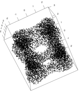
of the unknown shapeX, as illustrated by Figure 1.1. For X_n "close" enough to X, it is expected that

(14)

Figure 1.1: Point cloud sampled on the tangle cube inR3.

closeness between (compact) sets can described using various metrics. The traditional approach in

topological inference requires closeness between compact sets for the Hausdorff distance between X

and its approximation.

Generally speaking, point clouds in themselves do not carry any non-trivial topological or geometric structure. It is thus necessary to consider geometric structures on top of such point clouds in order to recover information about the shapes they approximate. In the most favorable situations, it is

possible to define such an approximation ˜Xn of the underlying object X that is homeomorphic to

X. In this case the topology of X can be described by the values of topological invariants on ˜Xn, as

for instance the number of components, the homotopy type, its Betti numbers (see below), etc. A weaker relation between topological spaces which however preserves many topological invariants is the

homotopy equivalence1.

The next section introduces the approximating models used for topological inference and more generally for TDA.

1.2 Approximating models for TDA: offsets and simplicial complexes

One natural strategy to infer topological information for an unknown shape from a point cloud is to

consider the offsets of the point cloud. For a point cloud X_n inRd (or in a metric space), the r-offset

of Xn is defined by Xr n“ ď xPXn Bpx, rq.

More generally, for any setX in a metric space pM, ρq, the r-offset Xr ofX is defined by

Xr

“ ď

xPX

Bpx, rq.

However, non-discrete sets such as offsets, and also continuous mathematical shapes like curves, sur-faces and more generally manifolds, cannot easily be encoded as finite discrete structures. Simplicial complexes are therefore used in computational geometry to approximate such shapes. These can be seen as generalizations of neighborhood graphs.

The definition of geometric simplicial complexes in Rd is now recalled, see also Figure 1.2(a). A

n-dimensional simplex s is the set of convex combinations of n+1 affinely independent points Xn “

1_{Given two topological spaces} _{X and Y, two maps f}

0, f1 : X Ñ Y are homotopic if there exists a continuous map

H: r0, 1s ˆ_{X Ñ Y such that for all x P X, Hp0, xq “ f}0pxq and Hp1, xq “ f1pxq. The two spacesX and Y are homotopy

equivalent if there exist two continuous maps f:_{X Ñ Y and g : Y Ñ X such that g ˝ f is homotopic to the identity map}

(15)

(a) The left set of simplices is a simplicial complexe whereas the right set of simplices is not.

(b) Delaunay complex in the plane and its empty ball charac-terization.

(c) one α-complex on the same set of points as for the Delaunay Complex.

Figure 1.2: Some geometric simplices inR2.

tx0, . . . , xnu. The points xi are called vertices. The simplices spanned by non-empty subsets ofXnare

called faces of s. Note that a point is a 0-simplex, a segment is a 1-simplex and triangle is a 2-simplex.

Definition 1. A geometric simplicial complex _{C is a set of simplices such that:}

• Any face of a simplex from C is also in C.

• The intersection of any two simplices s1, s2 PC is either a face of both s1 and s2, or empty.

A simplicial complex can also be seen as a combinatorial object consisting of subsets of the full vertex set of the complex. This remark motivates the following definition of abstract simplicial complexes.

Definition 2. Let Xn“ tx0, . . . , xnu be a finite set of elements. An abstract simplicial complexC with

vertex set Xn is a set of subsets of Xn such that:

• The elements of Xn belong to C;

• If s P C and H ‰ ˜s Ă s, then ˜s P C.

One important large family of constructions of simplicial complexes relies on the Delaunay com-plex. An exhaustive presentation of the Delaunay complex and its variants can be found for instance in Boissonnat et al. (2015). In this habilitation thesis, we only present the Delaunay complex and the

α-shape complex, see also Figures 1.2(b) and 1.2(c). Let Xn “ tx1, . . . , xnu be a point cloud of Rd

which is in general position2.

• A simplex rxi0, xi1, ¨ ¨ ¨ , xiks is in the Delaunay complex ofXnif and only if it has a circumscribing

ball empty of points ofXn.

• A simplex rxi0, xi1, ¨ ¨ ¨ , xiks is in the α-complex of Xn if and only if rxi0, xi1, ¨ ¨ ¨ , xiks is in the

Delaunay complex and the square radius of its circumscribing ball is at most α. The α-shape of

Xnfor scale parameter α is the set defined as the union of the simplices in the α-complex ofXn.

The Delaunay complex and the α-complex are both embedded inRdand they can be used for

approxi-mating an unknown shape in low dimension, typically for the Hausdorff metric. The α-complex can be also used for topological inference because it is homotopy equivalent to the union of the balls (Edels-brunner, 1993). However, as computation of the Delaunay complex is limited for practical reasons to very low dimensions, alternative constructions need to be considered for topological inference, like for

instance the Čech and Vietoris-Rips (or Rips) complexes. For a point cloud Xn“ tx0, x1, ¨ ¨ ¨ , xnu in

Rd _{and α ą 0, let Cech}

αpXnq and RipsαpXnq be the Čech and Rips complexes of scale parameter α

built on X_n (see also Figure 1.3):

• A simplex rxi0, xi1, ¨ ¨ ¨ , xiks is in the Čech complex CechαpXnq if and only if

Şk

j“0Bpxij, αq ‰ H.

(16)

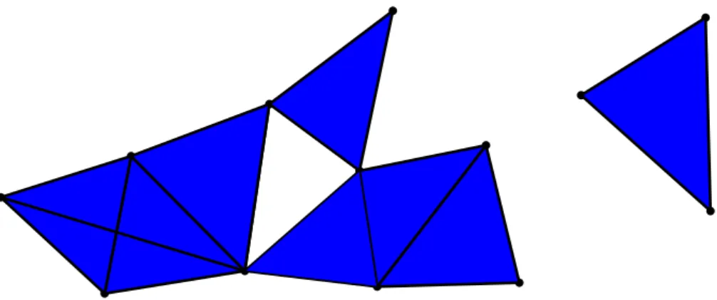
Figure 1.3: Left : Čech complex built on five points with a given scale parameter. Right: Rips complex built on the same points and with the same scale parameter α. The 2-simplices (or triangles) which

lie in the complex are filled in blue. The offsetXα_n is represented in pink.

• A simplex rxi0, xi1, ¨ ¨ ¨ , xiks is in the Rips complex RipsαpXnq if and only if }xij ´ xij1} ď

α for all j, j1

P t1, . . . , ku.

The definition of Čech and Vietoris-Rips complexes is not limited to the case of Euclidean spaces; they can be defined for a set of points in any metric space. In fact, the definition can be extended to any compact metric space (Chazal et al., 2014d).

The Nerve Theorem is a classical result in algebraic topology, see for instance Hatcher (2002).

It says that the offsets Xα_n of a point cloud Xn in Rd are homotopy equivalent to the Čech complex

CechαpXnq. This result opens the door to computational topology: the topology of the offsets can be

inferred from the topology of Čech complexes. For instance, Betti numbers on simplicial complexes (defined in the next section) can be computed with efficient algorithms. However, computation of Čech complexes quickly becomes difficult when the dimension increases. In practice, Rips complexes can also be used for encoding the topology of the offsets because of the following property:

Proposition 1. Let Xn be a set of points in Rn. Then, for any α ą 0:

Rips_αpXnq Ă CechαpXnq Ă Rips2αpXnq.

Simplicial complexes are usually parametrized by a scale parameter and the complete collection of simplicial complexes is called a filtration. More formally:

Definition 3. A filtration pCkqk“0,...,m of a finite simplicial complex C is an increasing sequence of

sub-complexes such that

• H “ C0 ĂC1Ă ¨ ¨ ¨ ĂCm “C,

• Ck`1“CkY sk`1 where sk`1 is a simplex of Ck`1.

For instance, the family of α-complexes is a filtration of the Delaunay complex. When simplicial complexes depend on a scale parameter α, by abuse of definition the filtration can also be indexed by

the scale parameter α: the filtration p_CαqαPr0, ¯αs is a filtration of the complexCα¯.

1.3 Simplicial homology

Homology is a mathematical formalism used to summarize connected components, holes, tunnels and voids in general in a topological space. The definition of homology on simplicial complexes, that is simplicial homology, is now briefly recalled. A complete presentation of simplicial homology and singular homology can be found for instance in Munkres (1984) or in Hatcher (2001).

In this habilitation thesis, we only consider simplicial homology on Z{2Z. In this framework,

simplicial homology has an obvious topological and geometric interpretation. Let _{C “ ts}1, . . . , sku be

a simplicial complex and k a dimension. A k-chain c is a formal sum of k-simplicial complexes in

(17)

Figure 1.4: Simplicial homology example: for this simplicial complex, β0“ 2 and β1 “ 1.

composed of the simplices whose coefficients are equal to one. A sum of two k chains c “ř aisi and

c1 _“_{ř b}

isi is defined by c ` c1 “

ř

pai` biqsi, where the sum between ai and bi is the sum inZ{2Z.

This can be seen as the symmetric difference of the two chains. With this addition operation, the set

of k chains on_{C, denoted by C}_kpCq, is an abelian group.

The boundary Bks of a k-simplex s is defined as the sum of its k ´ 1 faces and the boundary Bkc

of a k-chain c “ř aisi is defined as the sum of the boundaries of its simplexes. The elements of the

subgroup Zp :“ KerBk are called cycles: a k-cycle c is a k-chain with empty boundary. The elements

of the subgroup B_p :“ ImBk`1 are the k-boundaries: a k-boundary c is the boundary of a pk `

1q-chain. The main property of this construction is that the boundary of a boundary is necessarily zero.

Intuitively, the homology groups of_{C correspond to the voids of dimension k of the simplicial complex}

(see Figure 1.4 for an illustration).

Definition 4. The k-th homology group of _{C is the k-th cycle group modulo the k-th boundary group:}

Hp“ Zp{Bp. The k-th Betti number is the rank of this group: βk“ rank Hp.

In practice, one build a simplicial complex on a point cloud and Betti numbers appear as simple and interpretable topological signatures of the underlying shape on which the point cloud has been sampled. The notion of homology can be extended to general topological spaces by considering singular homology. This notion is beyond the scope of the thesis. We only mention here the key fact that singular homology is a topological invariant. This last property is, in some sense, the justification for using homology and Betti numbers computed on simplicial complexes for describing an unknown shape.

1.4 Topological inference and reconstruction procedures

This section gives a short presentation of topological inference results, see Boissonnat et al. (2015) for more details. There are two main facts relevant to topological inference results. The first is that, unsurprisingly, the difficulty in inferring the topology of a shape directly depends on its "regularity". There are several ways to quantify the regularity of a geometric shape. The second is that a complete theory of topological inference can be derived from the study of distance functions to compact sets.

For a compact set X in Rd, the distance function d_Xto X is the non-negative function defined by

d_Xpyq “ inf

xPX}x ´ y}.

Note that X is completely characterized by d_X since X “ d´1_X p0q. Moreover the r-offset Xr can be

defined by Xr “ d´1_X pr0, rsq. For some point y in the complement Xc of X, let Γpyq be the set of

points in X closest to y: Γ_Xpyq “ tx P X | }x ´ y} “ d_Xpyqu. The medial axis of Xc is defined by

MpXc

q “ ty PXc, |Γ_Xpyq| ě 2u. Several regularity properties of geometric shapes can be expressed as

(18)

X

Figure 1.5: This manifold is close to being self-intersecting and has a small reach.

Local feature size and reach

A local notion of regularity of a compact setX can be measured by the so-called local feature size. For

x PX, it is defined by lfs_Xpxq :“ d px,MpXcqq . The global version of the local feature size is the reach3

introduced by Federer (1959): κpXq “ infxPXclfs_X_{pxq. The reach is small if either} X is not smooth

or if X is close to being self-intersecting (see Figure 1.5) and the same remark is of course also true

locally for the local feature size. Amenta et al. (2000) show that a topologically correct reconstruction

of a surface smoothly embedded in R3 is possible from a point cloud, as soon as every point x P X

has a sample point at distance at most 0.06 lfs_Xpxq. However, this result cannot be applied when the

geometric shape has sharp edges because the local feature size vanishes on such edges. Weak feature size and its extensions

The weak feature size is a more flexible notion of regularity then the reach. It relies on the notion

of critical points for d_X. The function d_X is not differentiable everywhere but a generalized gradient

vector field_∇d_X for d_X can be defined as follows:

∇dXpxq “

#

x´θ

d_Xpxq if x RX

0 if x PX,

where θ is the center of the smallest closed ball enclosing Γpxq, see Figure 1.6.

Definition 5. A point x is a critical point of d_X if _∇d_Xpxq “ 0. A real c ě 0 is a critical value of d_X

if there exists a critical point x PRd such that d_Xpxq “ c. A regular value of d_X is a value which is not

critical.

The weak feature size of a geometric shape was introduced in Chazal and Lieutier (2007):

Definition 6. The weak feature size wfspXq of X is the infimum of the positive critical values of d_X.

If d_X does not have critical values then wfspXq “ `8.

Using the notion of critical point, Grove (1993) has shown that the sublevel sets of d_X are topological

submanifolds of Rd _{and that their topology can change only at critical points. Moreover, for}_{0 ă α ă}

β ă wfspXq, the offsets Xα and Xβ are isotopic4.

The following theorem is a typical example in the literature about topological inference of stability result. It shows that for some range of values of the scale parameter, two close compact sets have the same offset topology.

Theorem 1. [Chazal and Lieutier 2007] LetX and Y be two compact sets in Rd and let ε ą 0 be such

that dHpX, Yq ă ε, wfspXq ą 2ε and wfspYq ą 2ε. Then for any 0 ă α ă 2ε, Xα andYβ are homotopy

equivalent.

3

also called condition number

4

The notion of isotopy is stronger than homeomorphy to distinguish between spaces in Rd. An isotopy betweenX

andY is a continuous application F : X ˆ r0, 1s Ñ Rd such that F p.,0q is the identity map on_{X, F pX, 1q “ Y and for}

(19)

X

x

Γ

d

_X

(x)

θ

ρ

∇

X

(x)

Figure 1.6: Definition a generalized gradient for the distance function to a compact set.

However, the assumptions of Theorem 1 are not satisfied in the realistic case where an unknown

shapeX is approximated by a point cloud X_n. Indeed, the weak feature size of a finite point cloudX_n

is equal to half of the distance between the two closest points ofXn. In most cases, the two conditions

dHpX, Xnq ă ε and wfspXnq ą 2ε are not simultaneously satisfied.

To deal with this drawback, improvements to Theorem 1 have been proposed in particular in Chazal et al. (2009c). In short, a more general notion of regularity is introduced: the µ-reach, which interpolates between the minimum of the local feature (the reach) and the weak feature size. By considering this quantity as a measure of the regularity of the shape, it is shown in Chazal et al.

(2009c) that the homotopy type5 of X or at least that of its small offsets can be inferred from the

homotopy types of the offsets of an approximation of X. Here, the proximity required between X and

its approximation is in terms of the Hausdorff distance and also depends on the µ-reach of X.

A first probabilistic statement of topological reconstruction

In the paper Niyogi et al. (2008), it is shown that the homotopy type of Riemannian manifolds with reach larger than a given constant can be recovered with high probability from offsets of a sample on (or close to) the manifold. This paper is very important in the computational geometry literature since it was the first paper to consider the topological inference problem in terms of probability. The result of Niyogi et al. (2008) is derived from a retract contraction argument and on tight bounds over the packing number of the manifold in order to control the Hausdorff distance between the manifold and the observed point cloud. The assumption that the geometric object is a smooth Riemannian manifold is only used in the paper to control in probability the Hausdorff distance between the sample and the manifold, and not actually necessary for the "topological part" of the result. Regarding the topological results, these are similar to those of Chazal et al. (2009c) in the particular framework of Riemannian manifolds. Starting from the result of Niyogi et al. (2008), the minimax rates of convergence of the homology type have been studied by Balakrishnan et al. (2012) under various models, for Riemannian manifolds with reach larger than a constant. In contrast, a statistical version of Chazal et al. (2009c) has not yet been proposed.

1.5 Statistical approaches to TDA and topological inference

Until very recently, the theory on TDA and topological inference mostly relied on deterministic ap-proaches, as presented above. These deterministic approaches do not take into account the random nature of data and the intrinsic variability of the topological quantity they infer. Consequently, most

5

(20)

of the corresponding methods remain exploratory, without being able to efficiently distinguish between information and what is sometimes called the "topological noise".

A statistical approach to TDA means that we consider data as generated from an unknown dis-tribution, but also that the inferred topological features by TDA methods are seen as estimators of topological quantities describing an underlying object. Under this approach, the unknown object cor-responds to the support of the data distribution (or at least is close to this support). However, this support does not always have a physical existence; for instance, galaxies in the universe are organized along filaments but these filaments do not physically exist. A statistical approach to TDA is thus

strongly related to the problem of distribution support estimation and level sets estimation6 under the

Hausdorff metric, as suggested by the stability results presented in the previous section.

A large number of methods and results are available for estimating the support of a distribution in statistics. For instance, the Devroye and Wise estimator (Devroye and Wise, 1980) defined on a

sample X_n is also a particular offset of X_n. The convergence rates of both X_n and the Devroye and

Wise estimator to the support of the distribution for the Hausdorff distance is studied in Cuevas and

Rodríguez-Casal (2004) inRd. More recently, the minimax rates of convergence of manifold estimation

for the Hausdorff metric, which is particularly relevant for topological inference, has been studied in Genovese et al. (2012). There is also a large literature about level sets estimation in various metrics (see for instance Polonik, 1995; Tsybakov et al., 1997; Cadre, 2006) and more particularly for the Hausdorff metric in Chen et al. (2015). All these works about support and level sets estimation shine light on the statistical analysis of topological inference procedures.

The main goals of a statistical approach to topological data analysis can be summarized as the following list of problems:

Topic 1: proving consistency and studying the convergence rates of TDA methods.

Topic 2: providing confidence regions for topological features and discussing the significance of the estimated topological quantities.

Topic 3: selecting relevant scales at which the topological phenomenon should be considered, as a function of observed data.

Topic 4: dealing with outliers and providing robust methods for TDA.

The following chapters in this part of the thesis present our contributions to this statistical approach to TDA. The immediately following chapter gives a model selection method for automatically selecting a simplicial complex in a given filtration; this corresponds to Topic 3. Chapter 3 is about statistical methods for the estimation of persistence diagrams; the contributions of this chapter provide some answers to Topics 1 and 2. Chapter 4 is on the statistical analysis of a robust method for TDA based on the distance to measure. The contributions of this chapter correspond to Topics 1, 2 and 4.

(21)

Chapter 2 Model selection for simplicial

approximation

Given a point cloud Xn and a filtration of simplicial complexes pCαqαPA, choosing a convenient scale

parameter for topological inference or for reconstruction is not obvious. In this chapter, we address the problem of selecting a "convenient" simplicial complex as a model selection problem, as proposed in our paper Caillerie and Michel (2011). Our method relies on the theory of non-asymptotic model selection by penalization.

In this chapter, for q PN˚_{, the space}_Rq_{is equipped with the following normalized scalar product :}

@u, v PRq, xu, vyrqs:“ 1 q q ÿ i“1 uivi , (2.1)

and the associated norm is denoted } ¨ }rqs.

2.1 Geometric models

In the standard setting of topological inference in Rd, an unknown geometric object X embedded in

Rd _{is approximated from a point cloud} _X

n which points are observed in the neighborhood of X. We

then assume that the observed points X1, . . . , Xn satisfy

@i “ 1, . . . , n, Xi “ ¯xi` σξi with x¯i PX, (2.2)

where the original points x¯i are unknown and the random variables ξi are independent standard

Gaussian vectors ofRdand σ is the noise level. Let X “ pX₁t, . . . , X_ntqt be the vector of length q “ nd

containing all the observations Xi of the point cloudXn. We also define ¯x and ξ in the same way. We

consider the next equivalent statement of (2.2) in the space Rnd:

X “ ¯x ` σξ with x P¯ Xnd, (2.3)

where ξ is a standard Gaussian vector ofRnd.

In this work, we consider the geometric realization of a simplicial complex: by simplicial complexes we actually mean the support of the complexes by abuse of definition. For a given simplicial complex

C, the best approximating point of ¯x belonging toC minimizes the quantity t ÞÑ }t ´ ¯x}rnds. The least

square estimator (LSE) of ¯x associated to the complex_{C is then defined by}

ˆ

x:“ argmin_tPCn}X ´ t}2

rnds, (2.4)

where_Cn denotes the Cartesian product of _{C. For each i “ 1, . . . , n, let ˆx}i be the closest point of Xi

(22)

2.2 Selection of a simplicial complex in the filtration

Roughly speaking, a basic complex with only a few simplices will badly approximateX and the same

is true for ¯x, whereas a complex composed of too many simplices will tend to overfit the data. This

fact corresponds in statistics to the well known bias-variance trade off and it can be figured out by model selection methods.

LetP_¯_x be the distribution ofX in (2.3) and let pC_αqαPA be a filtration of simplicial complexes. We

denote by pCα :“ CαnqαPA the countable collection of Cartesian products of simplicial complexes and

by ˆxα the LSE estimator corresponding toCα, as defined in (2.4). The l2-risk of ˆxα is defined by

Rp¯x, αq “E¯x

´

}¯x ´ ˆxα}|2_rnds

¯ ,

whereE¯xis the expectation relative to P¯x. Ideally, we would like to choose the model αp¯xq minimizing

the risk: αp¯xq “ argmin_αPA_Rp¯x, αq. The model αp¯xq and the quantity ˆxαp¯xq, which is called oracle, are

both unknown in practice but it is considered as a benchmark for theory. One popular method to select an estimator in a given family is penalization. In our context, this procedure consists of considering

some proper penalty functionpen : α P_{A ÞÑ penpαq P R}` _{and of selecting}_{α minimizing the associated}_ˆ

l2 penalized criterion

critpαq “ }X ´ ˆxα}2_rnds` penpαq. (2.5)

The resulting selected estimator is denoted ˆxαˆ. Obviously, the main difficulty of this approach is to

choose a convenient penalty in order to select an estimator close to the oracle. For instance, the well

known AIC penalty is 2dασˆ2{n where ˆσ2 is an estimator of the noise variance and dα the "number of

parameters" estimated by ˆxαˆ. There is no obvious "number of parameters" associated to an estimator

ˆ

xC. The classical methods of penalization cannot be easily applied in our context.

A exhaustive theory of penalization with a non-asymptotic approach has been developed in the nineties, with the works of Birgé and Massart among others. This approach to model selection provides a penalty function leading to a oracle inequality for the penalized estimator. In Birgé and Massart (2001), such a non-asymptotic model selection result is obtained for collections of linear Gaussian

models, namely if the Cα’s were linear subspaces. For the case of nonlinear Gaussian models, Massart

(2007) shows that efficient penalties can still be defined by using the metric entropy (Section 4.4 in in this book). We follow this approach for selecting simplicial complexes.

For a k-simplex s inRd, let∆sbe the diameter of the smallest enclosing ball of s for the normalized

norm (2.1) inRd. A simplicial complex is said to be k-homogeneous if each one of its simplices is either

a k-simplex, or the face of a k-simplex of _{C. Then, for a k-homogeneous simplicial complex C in R}d,

let |C|k :“ p

ř

sPC`∆k_sq1{k and δC :“ infsPC`∆_s where C` is the subset of simplices of C of maximal

dimension k.

Let X be the observation vector with the distribution defined by (2.3). Let p_CαqαPA be a given

collection of k-homogeneous simplicial complexes in Rd and for each α P A let ˆxα be the LSE

corre-sponding to Cα“Cαn. Assume that there exist some weights wα such thatř_αPAe´wα “ Σ ă 8.

Theorem 2. [Caillerie and Michel 2011] Under the previous hypotheses, also suppose that for all α PA,

σ ď δCα c d k « 4κ ˜d ln4|Cα|k δCα `?π ¸ff´1 . (2.6)

There exist some absolute constants c1 and c2 such that for all η ą 1, if

penpαq ě η σ2 ˜ c1 k d « ln|Cα|k ? d σ?k ` c2 ff ` 4wα nd ¸ , (2.7)

then, almost surely, there exists a minimizer α of the penalized criterion (2.5) and the penalized esti-ˆ

mator ˆxαˆ satisfies the following risk bound

E¯x}ˆxαˆ ´ ¯x}2_rndsď cη „ inf αPA dp¯x,C n αq2` penpαq ( ` σ 2 ndpΣ ` 1q  (2.8)

where cη depends only on η and dp¯x, Cαnq :“ infyPCn

(23)

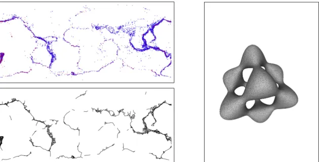
Figure 2.1: Landmarks in red and observed points in blue (top left) and selected α-complex (bottom left) for the seismic data. Selected α-complex for the Tangle Cube from noisy observations (right).

Condition (2.6) means that the complexes in the collection should not contain any k-simplexes with a diameter of the order of the noise level σ. This is natural since it would not be relevant to fit some simplices of this small scale on the observed data. This also means that the landmarks used to define the complexes should not be chosen too close to each other. The constant κ in the upper bound is an absolute constant which comes from Theorem 3.18 in Massart (2007).

The shape of the penalty function given by (2.7) is quite different than penalty shapes used in previous model selection works in the spirit of the results initiated by Birgé and Massart. The relevant

term in the penalty bound (2.7) is the "size measurement" ln |_Cα|k of the complex. The penalty also

depends on the weights wα. By analogy with the case of linear models (see Massart, 2007, p.91), we

can choose weights such that wα “ L ln |Cα|k with

ř

αPA 1

|Cα|Lk “ Σ ă 8, where L ą 0. The lower

bound (2.7) is then proportional toln |_Cα|k.

Note that bounds have no interest for the practice since they are surely far from being optimal. This theorem has to be considered from a qualitative point of view: the main contribution here is giving the penalty shape. This penalty shape does not directly depend on the geometric and topological properties of the complexes, but it is actually natural since the penalty is defined via the metric complexity of the simplicial complexes. However the method provides a "convenient scale" at which the geometric features have to be studied.

2.3 Applications

In practice, we consider α-complexes filtrations and we use the slope heuristics method presented in Chapter 6 to calibrate the penalty given in Theorem 2. In the particular case of graphs (k “ 1),

the termln |Cα|k exactly corresponds to the logarithm of the graph length, which is easy to compute.

Various applications are proposed in Caillerie and Michel (2011). Figure 2.1 illustrates two applications of the method: one on a seismic dataset and one for the reconstruction on the Tangle Cube.

We also apply the method for spectral clustering, a popular clustering method based on the spectral decomposition of a matrix associated to a similarity graph (see for instance von Luxburg, 2007). The algorithm requires the choice of a similarity function, and a type of graph to define a similarity graph.

A reasonable candidate for the similarity function is spx, yq “ expp´}x ´ y}2{p2σ2q. As to the graph,

the k-nearest neighbor graph and the ε-neighborhood graph are mostly used in practice. However, as explained in von Luxburg (2007), choosing ε or k is a difficult question. As far as we known, there is no completely data-driven method to do this choice and no theoretical results is available to help the user. Furthermore, this choice has a deep impact on the clustering, as illustrated by the example

(24)

-15 -10 -5 0 5 10 15 -15 -10 -5 0 5 10 15 -15 -10 -5 0 5 10 15 -15 -10 -5 0 5 10 15

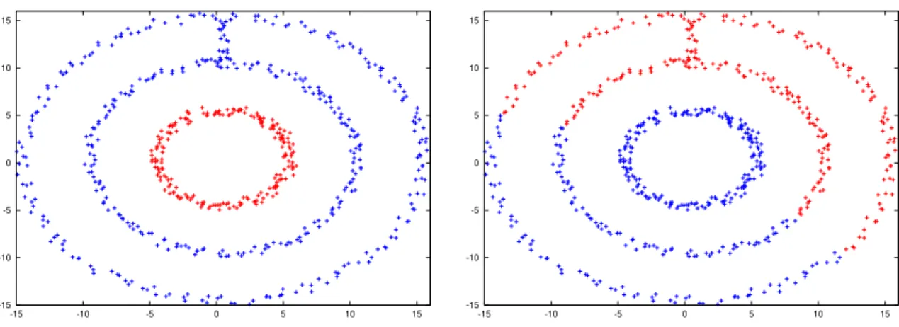
Figure 2.2: Data set (left) and 200 landmarks points (right).

-15 -10 -5 0 5 10 15 -15 -10 -5 0 5 10 15 -15 -10 -5 0 5 10 15 -15 -10 -5 0 5 10 15

Figure 2.3: Classical spectral clustering based on a k-nearest neighbor with k “ 25 (left) and k “ 30 (right) : the clustering depends on k.

-15 -10 -5 0 5 10 15 -15 -10 -5 0 5 10 15 -15 -10 -5 0 5 10 15 -15 -10 -5 0 5 10 15

Figure 2.4: Spectral clustering based on the graph selection for the initial data points (left) and the landmark points (right). The labels exactly corresponds to the expected clustering.

(25)

below (see Fig. 2.2 and 2.3). To answer this problem, we select a graph on the data according to our method and next we proceed the spectral clustering method with the selected graph, see Fig. 2.4.

2.4 Discussion and directions for future research

Selection of heterogeneous simplicial complexes.

This model selection method does not prevent us to deal with heterogeneous simplicial complexes. The problem is that no explicit shape for the penalty can be proposed in the heterogeneous case because the equation involved in the penalty definition is much more complicated than in the homogeneous case. This difficult and interesting question should be tackled in future works.

About the landmarks.

In practice, the hypotheses of Theorem 2 are not completely satisfied since the computed complexes necessary depend on the observed data and thus are "not fixed" as in the theorem statement. Our theoretical result can be considered as conditional to the landmark choice. Giving some mathematical results for the "random models" we use would be much more difficult among other things because the distribution of the landmarks cannot be easily specified.

Data driven topological inference.

Our method is a completely data driven model selection method for approximating a shape for the

`2 norm. By contrast, it does not directly answer to the problem of selecting a convenient scale in a

filtration for topological inference. One first direction of research would be to study the performance of our method on topological inference problems. It was noticed in Chapter 1 that topological inference can be derived from proximity for the sup norm metric. We intend to adapt Lepski’s methods for selecting a convenient scale in the filtration for the sup-nom metric.

Regarding the problem of estimating the homology of an underlying object, it must be noted that it is still not known how to build a reconstruction having the correct homology groups, in a data driven way. Consistency results have been proved by Niyogi et al. (2008) and more recently by Bobrowski et al. (2014), but these results are asymptotical. Consequently, the tuning of the scale parameters (or the bandwidth of the kernel estimators) proposed in these methods have no reason to be optimal in a non asymptotical point of view. Moreover they depend on geometric quantities which are unknown in practice. Finally, it is still unknown how to choose efficiently the scale parameters for a given point cloud of finite size. We would like to revisit the works of Niyogi et al. (2008) and Bobrowski et al. (2014) with model selection approaches in order to obtain a more data driven estimation method of the topology. The reach being a keystone quantity for all these methods, we currently study the estimation of this quantity from a statistical point, in a joint work in progress with F. Chazal, J. Kim, L. Wasserman and A. Rinaldo.

An alternative line of research about data driven topological inference would be to revisit the reconstructions results of Chazal et al. (2009c) with a statistical point of view. In this paper, a critical

function is introduced which describes the regularity of the distance function d_X and some insights

are also proposed on how to select the scale parameter in function of the critical function of the sample. Some stability results are also proven for the critical function. It would be interesting to

study the convergence of the "empirical critical function", that is the critical function for Xn and to

provide confidence regions for this last. This would open the door to a more "data driven" topological inference method, with statistical guarantees.

In the next chapter, we study the statistical aspects of persistent homology, an alternative approach to topological inference which consists in considering the complete filtration of simplicial complexes instead of considering only one particular scale.

(26)

Chapter 3 A statistical approach to persistent

homology on metric spaces

In this chapter, we study the statistical aspects of persistent homology, one of the most popular approach in topological data analysis. We saw in the previous chapters that inferring the exact topology of an unknown shape, or at least of its small of sets, require some geometric regularity assumptions on the shape which can be hardly checked in practice. We also noticed in the discussion section at the end of the previous chapter that, even if the shape is smooth, selecting a convenient scale (in the filtration of simplicial complexes) for inferring the homology from a given point cloud, is a tricky problem. On the contrary, persistent homology provides multiscale topological information and it is not restricted to particular smooth geometric objects ; it can be actually used for any compact metric space.

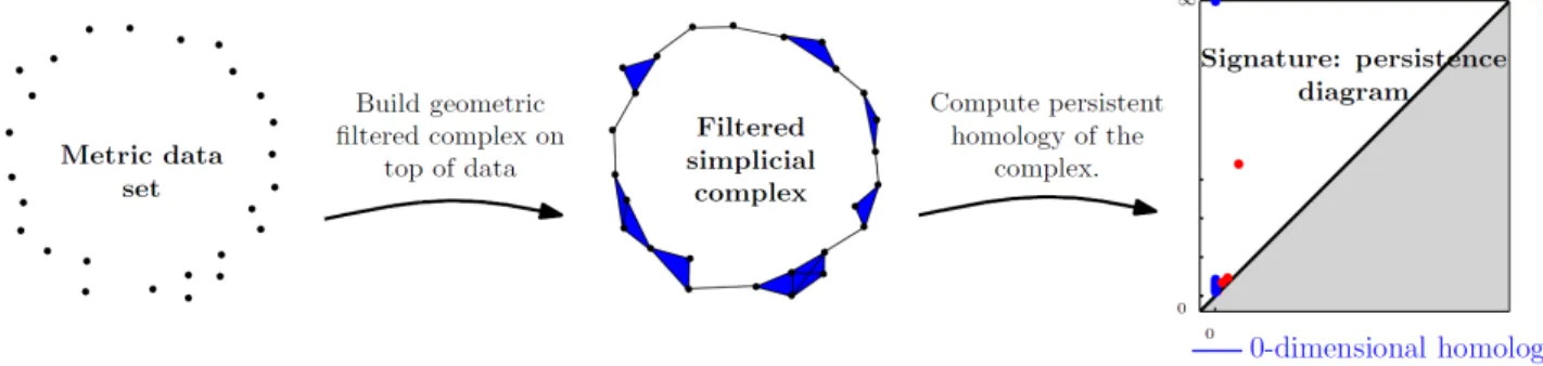
Generally speaking, persistent homology comes with a theory (Edelsbrunner et al., 2002; Zomoro-dian and Carlsson, 2005; Edelsbrunner and Harer, 2010; Chazal et al., 2012) and efficient algorithms to encode the evolution of the homology of families of nested topological spaces indexed by a set of real numbers. In most cases it is computed for a filtered simplicial complex built on top of the available data, see Fig. 3.1 for an illustration. The obtained multiscale topological information is then repre-sented in a simple way as a barcode, a persistence diagram (see Fig. 3.2) or a persistence landscape (see Fig. 3.3). These "topological signatures" are then used to exhibit and compare the topological structure underlying the data. Persistent homology has found applications in many fields, including neuroscience (Singh et al., 2008), bioinformatics (Kasson et al., 2007), shape classification (Chazal et al., 2009a), clustering (Chazal et al., 2013) and sensor networks (De Silva and Ghrist, 2007).

Several recent attempts have been made, with completely different approaches, to study persistence diagrams from a statistical point of view. One of the first statistical results about persistent homology has been given in a parametric setting in Bubenik and Kim (2007). They show that for data sam-pled on an hypersphere according to a von-Mises Fisher distribution (among other distributions), the

persistence diagrams of the density can be estimated with the parametric rate n´1{2_{. The approach}

of Mileyko et al. (2011) is completely different, it consists in studying probability measures on the space of persistence diagrams. Bubenik (2015) introduces a functional representation of persistence diagrams, the so-called persistence landscapes, allowing means and variance of persistence diagrams

(27)

connected component

cycle

birth death

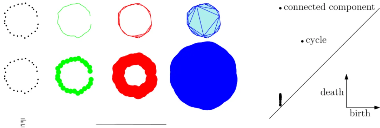
Figure 3.2: Left: an α-complex filtration, the sublevelset filtration of the distance function, and their common persistence barcode. Right: the corresponding persistence diagram.

to be defined, we will follow this approach in Section 3.3.

After recalling the main concepts about persistent homology, we present in this chapter the results of our papers Chazal et al. (2014b) and Chazal et al. (2014c) about rates of convergence of persistence diagram estimation. The third section is about the subsampling methods for persistent homology inference of our paper Chazal et al. (2015a).

3.1 Persistence diagrams and persistence landscapes

Filtrations on metric spaces. The simplicial complexes we consider in this chapter are built on top

of metric spaces. As noticed previously in the section 1.2, Čech filtrations and Vietoris-Rips filtrations can be defined in metric spaces. Those filtrations provide a convenient way to study the evolution of the topology of the union of growing balls or the sublevel sets of the distance to a compact, see Fig. 3.2.

In the following, the notation FiltpXq :“ pFiltαpXqqαPA denotes one of these filtrations on a compact

setX.

Persistent homology. An extensive presentation of persistence diagrams is available in Chazal

et al. (2012). We recall a few definitions and results needed for this chapter and we give the intuition

behind persistence. Given a filtration, the topology ofFiltαpXq changes as α increases: new connected

components can appear, existing connected components can merge, cycles and cavities can appear or be filled, etc. Persistent homology tracks these changes, identifies features and associates an interval

or lifetime (from αbirth to αdeath) to them. For instance, a connected component is a feature that

is born at the smallest α such that the component is present in FiltαpXq, and dies when it merges

with an older connected component. Intuitively, the longer a feature persists, the more relevant it

is. Given a filtration as above, we can compute theZ2-homology and we obtain the homology groups

HpFiltαpXq at each scale. These groups are also vector spaces pHpFiltαpXqqqαPA and the inclusions

FiltαpXq Ď FiltβpXq induce linear maps HpFiltαpXqq Ñ HpFiltβpXqq. In many cases, this sequence can

be decomposed as a direct sum of intervals, where an interval is a sequence of the form

0 Ñ . . . Ñ 0 Ñ_Z2 Ñ . . . ÑZ2 Ñ 0 Ñ . . . Ñ 0

(the linear maps Z₂ Ñ Z2 are all the identity). These intervals can be interpreted as features of

the (filtered) complex, such as a connected component or a loop, that appear at parameter α_birth

in the filtration and disappear at parameter αdeath. An interval is determined uniquely by these two

parameters. A feature, or more precisely its lifetime, can be represented as a segment whose extremities

have abscissae α_birthand α_death; the set of these segments is called the barcode of Filtp_{Xq. An interval}

can also be represented as a point in the plane with coordinates pαbirth, αdeathq, where the x-coordinate

(28)

Figure 3.3: We use the rotated axes to represent a persistence diagramDgm. A feature pαbirth, αdeathq P

Dgm is represented by the point pαbirth`αdeath

2 ,

αdeath´αbirth

2 q (pink). In words, the x-coordinate is the

average parameter value over which the feature exists, and the y-coordinate is the half-life of the feature. The cyan curve is the landscape λp1, ¨q.

Persistence diagrams. The set of points pαbirth, αdeathq representing the intervals is called the

persistence diagram and is denotedDgmpFiltpXqq in the following, see the right picture of Figure 3.2.

Note that the diagram is entirely contained in the half-plane above the diagonal∆ defined by y “ x,

since death always occurs after birth. Chazal et al. (2012) shows that this diagram is still well-defined

under very weak hypotheses, and in particular DgmpFiltpXqq is well-defined for any compact metric

space X (Chazal et al., 2014d). For technical reasons, the points of the diagonal ∆ are considered as

part of every persistence diagram, with infinite multiplicity. The most persistent features (supposedly the most important) are those represented by the points furthest from the diagonal in the diagram, whereas points close to the diagonal can be interpreted as (topological) noise.

Bottleneck distance. The space of persistence diagrams is endowed with a metric called the

bot-tleneck distance db. Given two persistence diagrams, it is defined as the infimum, over all perfect

matchings of their points, of the largest L8_{-distance between two matched points, see Fig. 3.4. The}

presence of the diagonal in all diagrams means we can consider partial matchings of the off-diagonal points, and the remaining points are matched to the diagonal. With more details, given two diagrams

Dgm₁ and Dgm₂, we can define a matching m as a subset ofDgm₁ˆ Dgm₂ such that every point of

Dgm₁z∆ and Dgm2z∆ appears exactly once in m. The bottleneck distance is then:

dbpDgm1,Dgm2q “ inf

matching m pp,qqPmmax ||q ´ p||8

.

Note that points close to the diagonal ∆ are easily matched to the diagonal, which fits with their

interpretation as irrelevant noise.

Persistence landscapes. The persistence landscape, introduced in Bubenik (2015), is a collection

of continuous, piecewise linear functions λ:_Z`_ˆ_{R Ñ R that summarizes a persistence diagram Dgm,}

see Fig. 3.3. To define the landscape, consider the set of functions created by tenting each point

p “ px, yq “ `αbirth`αdeath

2 ,

αdeath´αbirth

2

˘

representing a birth-death pair pαbirth, αdeathq P Dgm as

follows: Λpptq “ $ ’ & ’ % t ´ x ` y t P rx ´ y, xs x ` y ´ t t P px, x ` ys 0 otherwise “ $ ’ & ’ %

t ´ αbirth t P rαbirth,αbirth`α₂ deaths

αdeath´ t t P pαbirth`α₂ death, αdeaths

0 otherwise.

We obtain an arrangement of piecewise linear curves by overlaying the graphs of the functions tΛpup.

The persistence landscape ofDgm is a summary of this arrangement. To avoid minor technical

difficul-ties, we restrict our attention to persistence landscapes for metric spacesX such that pαbirth, αdeathq P

r0, T s ˆ r0, T s for all pαbirth, αdeathq P DgmpFiltpXqq, for some fixed T ą 01. Formally, the persistence

landscape ofDgmpFiltp_{Xqq is the collection of functions}

λDgmpFiltpXqqpk, tq “ kmax

p Λpptq, t P r0, T s, k PN, (3.1)

(29)

ε

∆

birth

death

Figure 3.4: Two diagrams at bottleneck distance ε.

where kmax is the kth largest value in the set; in particular,1max is the usual maximum function. We

set λ_DgmpFiltp_Xqqpk, tq “ 0 if the set tΛpptqup contains less than k points. For simplicity of exposition,

we use the notation λ_X to denote the landscape ofDgmpFiltpXqq, although the construction depends

on the chosen filtration.

Stability. Two compact metric spaces pX, ρq and p˜X, ˜ρq are isometric if there exists a bijection Φ :

X Ñ ˜X that preserves distances. One way to compare two metric spaces is to measure how far these two metric spaces are from being isometric. The corresponding distance is called the Gromov-Hausdorff

distance dGH (Burago et al., 2001). Intuitively, it is the infimum of their Hausdorff distance over

all possible isometric embeddings of these two spaces into a common metric space. A fundamental property of persistence diagrams, proven in Chazal et al. (2012), is their stability with respect to the Gromov-Hausdorff distance, one has

db ´ DgmpFiltpXqq, DgmpFiltp˜Xqq ¯ ď 2 dGH ´ X, ˜X¯. (3.2)

Moreover, ifX and ˜X are embedded in the same space pM, ρq then (3.2) holds for the Hausdorff distance

dH in place of dGH. From the definition of persistence landscape, we immediately observe that λpk, ¨q

is one-Lipschitz and thus a similar stability is satisfied for the landscapes.

Lemma 1. [Bubenik 2015] Let X and ˜X be two compact sets. For any t P R and any k P N, we have:

(i) λ_Xpk, tq ě λ_Xpk ` 1, tq ě 0.

(ii) |λ_Xpk, tq ´ λ_X˜pk, tq| ď dbpDgmpFiltpXqq, DgmpFiltp˜Xqqq.

3.2 Estimation of persistent diagrams on metric spaces

Assume that we observe n points X1. . . , Xn in a metric space pM, ρq drawn i.i.d. from some unknown

measure µ whose support is a compact set denotedXµ. The Gromov-Hausdorff distance allows us to

compareX_µwith compact metric spaces not necessarily embedded inM. In the following, an estimator

p

X of Xµ is a function of X1. . . , Xn that takes values in the set of compact metric spaces and which is

measurable for the Borel algebra induced bydGH.

Let FiltpXµq and Filtp pXq be two filtrations defined on Xµ and pX. Starting from (3.2) our strategy

consists in estimating the supportXµwith respect to thedGH distance. Note that this general strategy

of estimatingXµinK is not only of theoretical interest. Indeed, in some cases the space M is unknown

and the observations X₁. . . , Xn are just known through their pairwise distances ρpXi, Xjq, i, j “

1, ¨ ¨ ¨ , n. The use of the Gromov-Hausdorff distance then allows us to consider this set of observations

as an abstract metric space of cardinality n, independently of the way it is embedded in M. This

general framework includes the more standard approach consisting in estimating the support with

(30)

Let X_n :“ tX1, . . . , Xnu be a set of independent observations endowed with the restriction of the

distance ρ to this set. This finite metric space is a natural estimator of the support Xµ. In several

contexts discussed in the following, Xn shows optimal rates of convergence to Xµ with respect to the

Hausdorff distance.

The rate of convergence of X_n in Gromov-Hausdorff distance is obtained under the pa, bq-standard

assumption: for some constants a, b ą 0: for any x PXµ and any r ą 0,

µpBpx, rqq ě minparb,1q. (3.3)

This assumption has been widely used in the literature of set estimation under Hausdorff distance (Cuevas and Rodríguez-Casal, 2004; Singh et al., 2009).

Theorem 3. [Chazal et al. 2014b] Assume that the probability measure µ on M satisfies the pa,

bq-standard assumption, then for any ε ą 0:

P pdbpDgmpFiltpXµqq, DgmpFiltpXnqqq ą εq ď min

ˆ 2b aεbexpp´naε b q, 1 ˙ . (3.4) Moreover, lim sup nÑ8 ˆ n log n ˙1{b dbpDgmpFiltpXµqq, DgmpFiltpXnqqq ď C1

almost surely, and P ˜ dbpDgmpFiltpXµqq, DgmpFiltpXnqqq ď C2 ˆ log n n ˙1{b¸

converges to 1 when n Ñ 8, where C1 and C2 only depend on a and b.

Let_{P “ Ppa, b, Mq be the set of all the probability measures on the metric space pM, ρq satisfying}

the pa, bq-standard assumption on M:

P :“!µ on M | Xµ is compact and @x PXµ, @r ą 0, µ pBpx, rqq ě min

´

1, arb

¯)

. (3.5)

The next theorem gives upper and lower bounds for the rate of convergence of persistence diagrams. The upper bound is a consequence of Theorem 3, while the lower bound is established using Le Cam’s lemma.

Theorem 4. [Chazal et al. 2014b] For some positive constants a and b, sup µPPE rdb pDgmpFiltpXµqq, DgmpFiltpXnqqqs ď C ˆ log n n ˙1{b

where the constant C only depends on a and b (not on M). Assume moreover that there exists a non

isolated point x in M and consider any sequence px_nq P pMztxuqN such that ρpx, xnq ď panq´1{b. Then

for any estimator zDgm_n of DgmpFiltp_Xµqq:

lim inf nÑ8 ρpx, xnq ´1_sup µPP E ” dbpDgmpFiltpXµqq, zDgmnq ı ě C1

where C1 _{is an absolute constant.}

Consequently, the estimator DgmpFiltpXnqq is minimax optimal on the space Ppa, b, Mq up to a

logarithmic term as soon as we can find a non-isolated point in M and a sequence pxnq in M such

that ρpxn, xq „ panq´1{b. This is obviously the case for the Euclidean space Rd. One classical method

to obtain tight lower bounds with sup norm metrics is applying a Fano’s strategy based on several hypotheses (see for instance Tsybakov, 2009, Chapter 2). Applying this method is more difficult than it seems in our context. Indeed, the bottleneck distance makes tricky the construction of multiple hypotheses. However, in specific cases, we can obtain the matching lower bound with a more direct proof.

(31)

Theorem 5. [Chazal et al. 2014b] Consider p1₂,1q-standard measures on the unit segment r0, 1s. For

any estimator zDgm_n of DgmpFiltpXµqq:

lim inf nÑ8 sup µPPp1₂,1,r0,1sq n log nE ” dbpDgmpFiltpXµqq, zDgmnq ı ě C.

where C is an absolute constant.

It should be straightforward to extend this to measures on the cube r0, 1sb, as long as b is an integer,

with a lower-bound of Cbplog n_n q1{b. Note that this bound applies to the homology of dimension b. It is

possible that lower-dimensional homology may be easier to estimate.

Confidence regions. Theorem 3 can also be used to find confidence sets for persistence diagrams.

Such confidence sets depend on a and b which may be unknown and whose estimation is a difficult problem. Alternative solutions have been proposed in Fasy et al. (2014) using subsampling methods and kernel estimators among other approaches, in the specific context of smooth manifolds of an Euclidean space. Note that both Fasy et al. (2014) and our work start from the observation that persistence diagram inference is strongly connected to the better known problem of support estimation.

Persistence diagram estimation for nonsingular measures in Rk. Assume that µ is a

mea-sure on Rk with density f with respect to Lebesgue. Following Singh et al. (2009), assume (among

other assumptions) that in the neighborhood of the boundary BXµ of Xµ, f pxq ě C dpx, BXµqα. We

prove that DgmpFiltpXnqq converges in expectation to DgmpFiltpXµqq with a rate upper bounded by

plog n{nq1{pk`αq. Moreover, it can be shown that this rate is minimax over a convenient family of

densities with respect to the Lebesgue measure onRk.

Persistence diagram estimation for singular measures in RD. Let µ be a measure supported

on a smooth submanifold of RD with positive reach. Assume that µ has a density with respect to the

k-dimensional volume measure onXµ, which is lower and upper bounded onXµ. From Genovese et al.

(2012), we obtain that DgmpFiltp_Xnqq converges in expectation to DgmpFiltpXµqq with a rate upper

bounded by plog n_n q1{k both for support and persistence diagram estimation. Nevertheless, this rate is

not minimax optimal for support estimation, as shown by Theorem 2 in Genovese et al. (2012). The

correct minimax rate is actually n´2{k _{for both estimation problems.}

Additive noise. Consider the convolution model where the observations satisfy Yi“ Xi` εi where

X1, . . . Xn are sampled according to a measure µ as in the previous paragraph and where ε1, . . . , εn

are i.i.d. standard Gaussian random variables. We deduce from the results of Genovese et al. (2012) that the minimax convergence rates for the persistence diagram estimation in this context is upper

bounded by some rate of the order of plog nq´1{2_{. However, giving a tight lower bound for this problem}

appears to be more difficult than for the support estimation problem.

Persistence landscapes. According to the stability results given in Lemma 1, upper bounds on

the rates of convergence of the persistence landscapes directly derive from our results. A complete minimax description of the problem would also require to prove the corresponding lower bounds.

3.3 Subsampling methods for persistent homology

The time and space complexity of persistent homology algorithms is one of the main obstacles in applying TDA techniques to high-dimensional problems. To overcome the problem of computational costs, we propose in Chazal et al. (2015a) the following strategy: given a large point cloud, take several subsamples, compute the landscape for each subsample, and then combine the information. Indeed, contrary to persistence diagrams, persistence landscape can be averaged in a straightforward way.

As in the previous section, a probability measure µ is defined on a metric space pM, ρq and the

A Statistical Approach to Topological Data Analysis

HAL Id: tel-01235080

https://tel.archives-ouvertes.fr/tel-01235080

A Statistical Approach to Topological Data Analysis

Bertrand Michel

To cite this version:

A Statistical Approach to Topological

Data Analysis

soutenue le 24 novembre 2015

Remerciements

Foreword

Contents

Part I

Statistical aspects of topological data

analysis

Chapter 1

Introduction

1.1

Topological data analysis

1.2

Approximating models for TDA: offsets and simplicial complexes

1.3

Simplicial homology

1.4

Topological inference and reconstruction procedures

X

X

x

Γ

d

(x)

θ

ρ

∇

(x)

1.5

Statistical approaches to TDA and topological inference

Chapter 2

Model selection for simplicial

approximation

2.1

Geometric models

2.2

Selection of a simplicial complex in the filtration

2.3

Applications

2.4

Discussion and directions for future research

Chapter 3

A statistical approach to persistent

homology on metric spaces

3.1

Persistence diagrams and persistence landscapes

ε

∆

birth

death

3.2

Estimation of persistent diagrams on metric spaces

3.3

Subsampling methods for persistent homology