HAL Id: tel-01358280
https://tel.archives-ouvertes.fr/tel-01358280v2
Submitted on 1 Sep 2016HAL is a multi-disciplinary open access
archive for the deposit and dissemination of sci-entific research documents, whether they are pub-lished or not. The documents may come from teaching and research institutions in France or abroad, or from public or private research centers.
L’archive ouverte pluridisciplinaire HAL, est destinée au dépôt et à la diffusion de documents scientifiques de niveau recherche, publiés ou non, émanant des établissements d’enseignement et de recherche français ou étrangers, des laboratoires publics ou privés.
Jeremie Saives
To cite this version:
Jeremie Saives. Blackbox Behavioural Identification of Discrete Event Systems by Interpreted Petri Nets. Automatic Control Engineering. Université Paris-Saclay, 2016. English. �NNT : 2016SACLN018�. �tel-01358280v2�
NNT : 2016S
B
Ide Thèse prés Compositi M. Basile Fra M. Lopez Lu M. Alla Hass M. Riera Ber M. Lesage Je M. Faraut Gr SACLN018D
Science
Sp
Blackbox
entification entée et sou ion du Jury ancesco uis Ernesto sane rnard ean-Jacques regoryT
DE L’U
p
s et Techn
pécialité E
M
x Behavio
Comporte utenue à Cac y : Professeur, U Professeur, C Professeur, G Professeur, U Professeur, E MdC, ENS CTHESE
UNIVER
préparée
ÉCOLE D
nologies d
lectroniqu
Monsieu
ural Iden
Inter
mentale “B par Résea chan, le 30 j Univ. di Salern Cinvestav Gua GIPSA-Lab, Fr URCA-CReST ENS Cachan – Cachan – LURDE DO
RSITE P
e à l’EN
DOCTORA
de l'Inform
ue, Electro
Parur Jérém
ntification
rpreted Pe
Boîte-noire aux de Petr juin 2016. no, Italy adalajara, Mex rance TIC, France – LURPA, Fra RPA, FranceOCTORA
PARIS-S
NS Cach
ALE N° 5
mation et d
otechnique
mie SAIV
n of Discre
etri Nets
” des Systè ri Interprét Rapporte xico Rapporte Président Examinat ance Directeur Co-encadAT
SACLA
han
580
e la Comm
e, Automa
ES
ete Event
èmes à Evén tés ur ur t teur r de thèse drantAY,
munication
atique
t Systems
nements Dn
by
iscretsDuring these last three years, I was a member of the world of research, developping contributions and pushing further away the limits of science. When I came to ENS Cachan seven years ago, I had teaching as sole purpose; I hope now that I can combine teaching and research in my future career.
Retrospectively, this thesis is an experience to be proud of, and I am grateful to the people who made it possible. Notably, I want to thank first Jean-Jacques Lesage, who took me under his wing in the last years. His teachings and advice helped me become a better scientist. To complete the team, Gregory Faraut was always available to cheer me up, discuss ideas and help me proof test some of them. I wish him an accomplished scientific career. I would also like to thank Jean-Marc Roussel for bringing me to the field of discrete automatic, being actually the first milestone who led to this thesis.
Joyful was the ending, and I would like to thank my jury for reviewing this work. Francesco Basile came all the way from Italia, and I thank him for his enthusiasm regarding DES identification. Ernesto Lopez-Mellado provided helpful advice for the formalization, and I thank him also for inviting me to Mexico two years ago. Finally, Hassane Alla and Bernard Riera showed as well a lot of interest, and I thank them for their sympathy.
Escaping the routine was made possible by colleagues, PhD and Master students, friends and geeks alike. I thank all the LURPA for the environment, and the good mood. Resting now on the shoulders of my coffee-mate Laureen, the CIVIL is a wonderful committee which makes everyone feel integrated, and the hard days easier. I’m happy to have directed it, see it now in good hands, and thank all its members, past and present. Especially Julien, my dear neighbour from Office 18, who supports my rantings and my cats. Lorène and Fabien, who arrived with me, and with whom I shared the difficulty of writing. But also Matthias, Kevin, Sylvain and all the younglings.
My roommate, Blandine, who shared a sinusoidal mood with me during this last year. My former roomate, Benjamin, who came from far away to see my defence.
It is said that being a teacher in a classroom is like being an actor on stage. I thank the LiKa, my improv team, among which I developped acting skills and gained confidence. To Marc, Simon, Pat, Mathilde, and a lot of others I might forget.
Ending these acknowledgements could only be done by thanking my parents for their continuous support, and I am afraid there is not enough space here to be exhaustive.
Table of contents iii
List of figures vii
List of tables xiii
Introduction 1
1 Identification of Discrete Event Systems 5
1.1 Background on Discrete Event Systems . . . 5
1.1.1 Definition . . . 5
1.1.2 Reactive DES and event generators . . . 7
1.1.3 Formalism: Classical models . . . 8
1.2 Identification of a DES: Problem Statement . . . 14
1.2.1 Systems of Interest . . . 15
1.2.2 Incompleteness of the observation . . . 19
1.2.3 Problem Statement . . . 21
1.2.4 Identification for reverse engineering . . . 21
1.3 Identification in the literature . . . 22
1.3.1 Origin: early computer science approaches . . . 22
1.3.2 Identification by Automata. . . 23
1.3.3 Identification by Petri Nets . . . 27
1.4 Conclusions and positioning . . . 39
2 Blackbox behavioural identification of a reactive automated system 41 2.1 Two behaviours: Observable and Unobservable . . . 41
2.1.1 Event types . . . 41
2.1.2 Framework of the method . . . 43
2.1.3 Illustrative example: Sorting system . . . 44
2.2 Identification of the observable behaviour . . . 45
2.2.1 Building output firing functions . . . 45
2.2.2 Construction of the transitions and observable places . . . 48
2.2.3 Determination of the firing sequence . . . 51
2.3 Inference of the unobservable behaviour . . . 51
2.3.2 Computing unobservable places . . . 54
2.3.3 Verification of the net . . . 56
2.4 Discussion and proposed improvements . . . 56
2.4.1 Scalability and concurrency . . . 57
2.4.2 Limits of the unobservable behaviour discovery . . . 58
3 Scalability of the observable behaviour construction 61 3.1 Illustrative system: the MSS . . . 61
3.1.1 Presentation . . . 61
3.1.2 Data collection . . . 63
3.2 Resynchronization of asynchronous events in concurrent systems and con-sequences . . . 64
3.3 Filtering of the causality matrix . . . 67
3.3.1 Design of the filter . . . 67
3.3.2 Application . . . 71
3.4 Transitions reduction . . . 73
3.4.1 Replacement of spurious transitions . . . 73
3.4.2 Application . . . 79
3.5 Conclusions . . . 84
4 Discovery of the unobservable behaviour 85 4.1 Problem statement . . . 85
4.2 Theoretical background. . . 86
4.2.1 From the firing sequence to admissible places. . . 86
4.2.2 Complexity of finding admissible places . . . 90
4.2.3 Intermediate conclusions . . . 93
4.3 Assessing the quality of a net . . . 94
4.3.1 Quality metrics . . . 95
4.3.2 Importance of understandability . . . 97
4.4 Discovery in practice . . . 100
4.4.1 Partitioning of the search space . . . 100
4.4.2 Exploration strategy . . . 103
4.4.3 Stopping criterion . . . 104
4.4.4 Algorithmic application . . . 105
4.5 Extensions . . . 106
4.5.1 Implicit places and consequences . . . 107
4.5.2 Reduction of the algorithmic cost . . . 109
4.6 Practical examples . . . 112
4.6.1 Unobservable behaviour only. . . 112
4.6.2 Complete approach . . . 114
4.8 Conclusion . . . 120
5 Automated partitioning for distributed identification 123 5.1 Statement of the partitioning problem . . . 123
5.1.1 Objective of the partitioning . . . 123
5.1.2 Related work . . . 127
5.1.3 Mapping I/Os and observable fragments . . . 130
5.1.4 Final formulation . . . 134
5.2 Partitioning by agglomerative hierarchical clustering. . . 138
5.2.1 Similarity and affinity of subsystems . . . 138
5.2.2 Limited clustering. . . 142
5.2.3 Results and interpretation . . . 144
5.3 Conclusion . . . 149
Conclusion and outlooks 153 Bibliography 157 A Assessing the quality of an identified Petri net 173 A.1 Precision . . . 173
A.2 Complexity metrics . . . 175
A.2.1 Structural Complexity . . . 176
A.2.2 Dynamic Complexity . . . 178
1.1 Overview of a closed-loop logical system, with its inputs U, its outputs
Y, and its state variables X . . . 6
1.2 [Cassandras and Lafortune, 2008] An example of a state trajectory of a DES. . . 7
1.3 A spontaneous event generator (a). A closed-loop system consisting in two reactive systems, interacting through their I/Os (b) . . . 8
1.4 A closed-loop system consisting in two reactive systems, seen as an event generator . . . 8
1.5 An example of a DFA. . . 10
1.6 An example of a PN . . . 12
1.7 An example of an IPN . . . 14
1.8 The cyclic behaviour of a Programmable Logic Controller, including the passive observation . . . 16
1.9 An observation of the process controlled illustrating the functioning of the PLC . . . 17
1.10 An illustration of the synchronization effect. . . 18
1.11 An illustration of a delayed output event . . . 19
1.12 [Roth et al., 2009a] Evolution of the number of observed words of length n over production cycles h . . . 20
1.13 [Roth, 2010] Observed languages over a hundred production cycles . . . . 20
1.14 [Prähofer et al., 2014] Left: A flow chart of a function block of the PLC, with the paths numbered. Right: A trace and its representation as a FSM 24 1.15 [Klein, 2005](a) The identified NDAAO after the treatment of the se-quences; (b) The simplified model after merging of equivalent states . . . 25
1.16 From [Hiraishi, 1992]: (a)The finite acceptor and (b) the PN deduced from it. . . 27
1.17 Illustration of a region, and its elementary net equivalent . . . 29
1.18 [Giua and Seatzu, 2005] Two free-labelled, generalized nets identified from solving ILP . . . 30
1.19 [Cabasino et al., 2014](a)Nominal net; (b) Faulty net with two silent transitions . . . 31
1.21 [Van der Aalst, 2013a] Positioning of the three main types of process
mining: discovery, conformance and enhancement . . . 33
1.22 [Van der Aalst et al., 2004] The net mined by the α-algorithm from the
log {ABCD, ACBD, AED} . . . 35
1.23 [Meda-Campana and Lopez-Mellado, 2001] 6 nets incrementally
com-puted from the observed output sequences . . . 36
1.24 [Estrada-Vargas et al., 2014](a) Basic identified model; (b) Model after
merging; (c) Model after concurrency simplification; (d) IPN model with
observable places . . . 38
1.25 Left: Unobservable part (machine behaviour). Right: Observable part
(signals) . . . 39
2.1 Data collection, then construction of an IPN in two steps . . . 44
2.2 Illustrative example: a package sorting system . . . 44
2.3 Matrices computed for the sorting system. Left: Direct Causality Matrix,
Right: Indirect Context Matrix . . . 47
2.4 Elementary observable fragments constructed from the firing functions . 49
2.5 Example of the creation of a new transition, by choosing the right input
conditions . . . 49
2.6 Example of the creation of a new transition, based on a simultaneous
output events observation . . . 50
2.7 Result of the first step for the sorting system: the observable part . . . . 50
2.8 Structures that represent ta < tb: a) shows a causal relationship whereas
b) shows a concurrent relationship. . . 52
2.9 a)Choice and b)parallelism after the firing of tk . . . 55
2.10 The non-observable part of the IPN computed for the sorting system . . 55
2.11 (a) The unobservable part, corrected by the token-flow equation; (b) The
final IPN with both interpretation layers . . . 57
2.12 (a) The observable part of the net; (b) The net identified ; (c) A net that
satisfies the problem . . . 59
2.13 A non free choice net with two memory places . . . 59
3.1 A picture of the MSS in the LURPA, and of the workpieces (gears and
bearings) processed.. . . 62
3.2 Scheme of the MSS, decomposed in 4 stations and 11 subsystems . . . . 62
3.3 Observed language of the MSS over 20 production cycles, for n = 1, 2 . . 63
3.4 Two concurrent processes observed asynchronously . . . 64
3.5 Two concurrent processes spuriously observed synchronously . . . 65
3.6 (a) Observable part identified for two concurrent processes with spurious
transitions (b) Simplified desirable model . . . 66
3.7 MSS transition occurences . . . 66
3.9 Result of the Filter on the DCM of the MSS. Grey cells correspond to
validated non-empty cells, and black cells to noise. . . 71
3.10 Efficacity of the filter: better denoising for column sums close to one. . . 72
3.11 Principle of the reduction: remove transitions and replace in S . . . 73
3.12 Increase of the permissivity of transitions by OEFF labelling . . . 74
3.13 Example of an observable fragment, with t1 reducible by [t4, t5]. . . 75
3.14 An observable fragment; only the unrelated input events are shown in the firing functions . . . 76
3.15 Non-unicity of minimal reductions illustrated by t5 . . . 78
3.16 Observable Behaviour of the MSS pre-reduction: one single spaghetti fragment . . . 82
3.17 The result of the reduction for the MSS: 30 observable places and 101 transitions. 13 observable fragments and 24 isolated transitions. . . 83
3.18 Observed language of the MSS expressed on the transitions, for n = 1, 2, 3 84 4.1 An unobservable PN built from S using mutual dependencies. . . 88
4.2 A PN structure composed of two places pij and pji for Σi = {t1i, . . . , tmi }, Σj = {t1j, . . . , tnj}. t1i is the first transition fired. . . 89
4.3 Two net solutions, built with different sets of admissible places . . . 91
4.4 Visualisation of the complexity of the problem . . . 94
4.5 A system consisting of two chariots and a gripper . . . 97
4.6 Observable part of the system. 5 outputs and 9 observable transitions . . 98
4.7 (a) A simple solution, with a lot of exceeding language ; (b) A complex solution, with no exceeding language up to n = 6 . . . 99
4.8 Visual representation of the partition of (2T − {∅})2 6∩. . . 102
4.9 Size of the cell Dδ of the search space depending on δ, plotted for different values of |T |. Y scale is logarithmic. . . 104
4.10 The chariots example: (a)Observable part; (b)Initial net for the explo-ration; (c)Net identified at the end of the limited exploexplo-ration; (d)Net identified by a full exploration . . . 106
4.11 An example of a net (a), after deletion of implicit places (b) . . . 107
4.12 Results of the identification of Example 4.7. . . 108
4.13 Vertical propagation of the domination relationship . . . 111
4.14 Example 4.9: (a) Net discovered for D2; (b) Net discovered for D3 . . . . 113
4.15 Example 4.10: the initial marking is unreachable after any firing.. . . 113
4.16 Example 4.11; there are two backward loops in the main process t0 −→ t1114 4.17 Example 4.12: 5 fully concurrent processes, synchronized by m . . . 114
4.18 Example 4.13: (a)Observable part; (b)Solution D2; (c)Solution D4 . . . . 115
4.19 Extended chariots example, with its observable behaviour . . . 115
4.20 The resulting net after the exploration of D2.. . . 116
4.22 Monolithic IPN model obtained after the exploration of δ = 2. 5 tran-sitions and two fragments remain unconnected to the remainder of the net . . . 121
5.1 Principle of the distributed approach, based on a partition of the system. 124
5.2 Identified net for SUBk consisting in either 1 output or 1 input . . . 126
5.3 Shape of the Pareto frontier of optimal solutions of the cover problem . . 126
5.4 (a) The NDAAO and (b) the IPN built from SUBk = {u1, Y1} . . . 128
5.5 Overview of the partitioning approach from [Schneider, 2014] . . . 129
5.6 Mapping of an observable fragment and isolated transitions on the
differ-ent I/O sets . . . 131
5.7 Sharing a connected input between two fragments and two isolated
tran-sitions. . . 132
5.8 Possible unobservable behaviour for a Type 2 Block . . . 134
5.9 Location of the blocks on the MSS . . . 134
5.10 Overview of the distributed approach, partitioning taking place after the
construction of the observable model . . . 135
5.11 The 21 blocks computed for the MSS . . . 137
5.12 Similarity table and Affinity graph deduced for Example 5.4 . . . 139
5.13 (a) Evolution of the affinity graph along the clustering; (b) Hierarchical
representation . . . 141
5.14 Successive affinity graphs, first run of the clustering, with |T |Lim= 9 . . 145
5.15 Successive affinity graphs, second run of the clustering, with |T |Lim = 18 146
5.16 Location of the six computed subsystems on the MSS, |T |Lim = 18 . . . . 146
5.17 Location of the six computed subsystems on the MSS, tLim = 20s . . . . 147
5.18 Succesive affinity graphs computed for the MSS, tLim = 20s . . . 148
5.19 Evaluation of different partitions computed with the clustering approach 149
5.20 IPN identified for SSY S1, biggest subsystem of the MSS . . . 150
5.21 IPNs identified for the remaining subsystems of the MSS . . . 151
Fr.1 Principe du filtre : Annuler les cases de la matrice correspondant à des
observations parasites. . . 169
Fr.2 Principe de la réduction : Suppresion des transitions, et remplacement
dans S . . . 169
Fr.3 Motif projeté caractérisant une mutuelle dépendance, et places associées. 170
Fr.4 Deux RdPI identifiés pour le même système : (a) est simple, mais génère
plus de langage excédentaire que (b) . . . 170
Fr.5 Exemple de l’approche par clustering : Evolution d’un graphe d’affinité
(a), et construction de la hiérarchie (b) . . . 171
Fr.6 Localisation des six sous-systèmes obtenus par time-clustering sur la MSS,
A.1 First row: N identified for S, and its exceeding language; Second row: N’
identified for S’, and its exceeding language. . . 174
A.2 The net N identified and its exceeding language according to Definition A.2175
A.3 (a) A simple solution, with a lot of exceeding language ; (b) A complex
solution, with no exceeding language up to n = 6 . . . 176
1.1 Similarity between closed-loop systems and IPN . . . 40
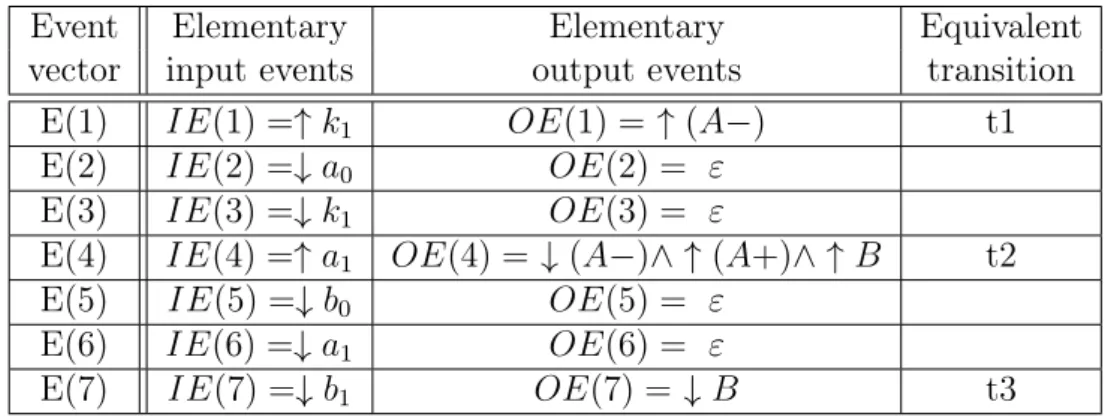
2.1 Elementary description of the first event vectors . . . 45
2.2 Firing functions computed for the sorting system . . . 48
2.3 Translation into the firing sequence of the first vectors of E . . . 51
3.1 DCM of two concurrent processes . . . 65
3.2 Non empty cells of the column DCMi,1Y 04_0 . . . 67
4.1 Evaluation of the precision and simplicity metrics on the discovered nets for the chariots. . . 117
4.2 Evaluation of the simplicity metrics on the discovered nets for the MSS. . 118
A.1 Comparison of structural complexity metrics on Example 4.5 . . . 178
System modelling has become a preponderant task in engineering, namely in the field of automatic control, where models are extensively used to find optimal control laws. Iden-tification consists in building a mathematical model of a system from its observation; namely, parametric identification is widely spread to build models of continuous-time systems described by differential equations. However, Discrete Event Systems (DES), described by state-based models whose evolutions are triggered by events, are often modelled from expert knowledge only. DES identification has received more and more interest over the last decade. The objective of this thesis is to contribute to its develop-ment, in order to make identification a viable alternative to expert modelling.
Identification is an experimental approach by nature, requiring to observe a real system during its operation. The experimental setup implies physical and technological constraints, which must be taken into account by identification algorithms. Namely, the nature of the input/outputs, the cyclicity of the controller or the impossibility to achieve complete observation are challenges to be accepted. Another challenge is to develop scalable algorithms, in order to deal with systems of realistic sizes, despite the state-space explosion issue quite usual for concurrent DES.
Models are designed for a purpose, be it either simulation, performance evalua-tion, control, diagnosis, dysfunctional analysis... Identified models should be designed likewise, and identification algorithms concieved for a given purpose. Model-based fault diagnosis has been the key motivation for a series of theses ([Klein, 2005][Roth, 2010][Schneider, 2014]). The resulting models, automata, are especially efficient for diagnosis. However, they lack the semantics to offer an explicit vision of complex be-haviours such as concurrency, or input/output causalities. This thesis is thus dedicated to reverse-engineering. The aim is to produce compact models, easily readable, in order for an engineer to understand the operations performed by the system.
The focus of this thesis is set on closed-loop systems consisting in a plant and a con-troller. Sensors and actuators of the plant are respectively the logical inputs and outputs of the controller, typically a Programmable Logic Controller (PLC). These controllers are widely used in manufacturing systems for their robustness to hostile environments, and their reactivity to sensor events. In this thesis, the identification is blackbox, i.e. no knowledge about the internal variables of the system is available, and passive, i.e. the observed data consists only in the values of the inputs/outputs, recorded during the operation of the system.
the direct causal input/output evolutions of the DES, and an unobservable part, in which are agregated memory effects, timed behaviours or sequential evolutions of the internal state variables of the system. Interpreted Petri Nets (IPN) offer the semantics to visualize both parts in a single graphical model. For reverse engineering, these models should be compact and as simple as possible.
To achieve this goal, an approach in two steps was proposed in a previous the-sis [Estrada-Vargas, 2013]. The observable, then unobservable parts of the model are built successively. The first step is performing, building fragments expressing the in-put/output causalities. These fragments are then connected in the second step by adding the unobservable part, leading to a monolithic model. The method was succesfully ap-plied to small systems, but several difficulties appeared when bigger, concurrent systems are considered. Direct causalities on one hand, and concurrency in the unobservable be-haviour on the other hand, become harder to discover.
The contributions of this thesis aim therefore at improving the scalability of the approach, and are the following:
• Improve the monolithic approach by:
– Limiting the effects of concurrency in the construction of the observable part.
– Developping a new approach for the discovery of the unobservable part.
• Propose a distributed approach, to split the system into subsystems when mono-lithic models become too big to be apprehended or computed.
This document is organized as follows:
Chapter 1 presents the formalisms used through the thesis, namely IPNs, the systems considered, and the problems and challenges related to DES identification. A review of the state of the art is proposed, from the first techniques of computer science to the DES-related works of the last years.
Chapter 2 resumes the approach in two steps developed in [Estrada-Vargas, 2013], in which the remainder of the thesis takes its roots. The construction of the observable behaviour, based on a probabilistic framework, and the discovery of the unobservable behaviour, based on numerous rules, are successively exposed and illustrated. The new challenges offered by concurrency to both steps are exposed; these challenges are taken up by the contributions presented in this thesis.
Chapter 3 develops the improvement of the observable step towards more scalability. An absorbing filter is designed to get rid of spurious correlations between inputs and outputs, observed due to the concurrency of the system coupled with the synchronization of the controller, and falsely interpreted as causalities. Irrelevant transitions created by the same phenomenon are filtered and reduced as well. A real system available at the LURPA is introduced in this chapter. Its reasonable size (73 I/Os) makes it a good illustration of the scalability improvements presented throughout in this thesis.
the identified model, and ensure its fitness, as the observed behaviour is fully repro-duced. Due to state-space explosion, a heuristic is proposed to perform the discovery in practice. This heuristic is designed to reduce the structural complexity of the resulting model, desirable quality of a model dedicated to reverse-engineering.
Finally, Chapter 5 proposes a distributed approach, to be employed when monolithic models become too big to be computed, and hard to understand on top of it. The distribution occurs after the computation of the observable behaviour; the observable fragments are used as an initial partitioning of the system, and a hierarchical clustering algorithm is proposed. The fragments are merged while ensuring that the resulting subsystems are satisfyingly modelled, until a computation time threshold is reached. The result is a set of distributed models, easier to compute, and easier to read due to their reduced size, thus fitting the objective.
1
Identification of Discrete Event
Systems
Introduction
The research presented in this thesis deals with Identification of Discrete Event Systems, i.e. the construction of mathematical models from observed data, collected during the operation of the real system. The aim of this research is more specifically to provide compact models exhibiting the reactive behaviour of the observed system.
First, Discrete Event Systems are defined in Section 1.1, and the modelling for-malisms are recalled. Then, the systems of interest, with their technological constraints, are presented, leading to the statement of the problem dealt with in this thesis (Sec-tion 1.2). Numerous works dealing with Discret Event Systems Identification are then reviewed in Section 1.3. Finally, Section 1.4 concludes on the choice of model adapted to the objective, and presents the contributions of this thesis.
1.1
Background on Discrete Event Systems
1.1.1 Definition
First, an informal description of the behaviour of systems is given. Generically speaking, a dynamical system can be associated to input variables U = {u1, u2, . . . , u|U|}
and output variables Y = {y1, y2, . . . , y|Y|}. Input variables are stimuli that provoke a
response through the output variables.
The output variables might depend only on the values of the input variables, i.e. ∀j, yj = f (u1, . . . , u|U|)). Namely, continuous-time systems are often described by
or-dinary differential equations (y = f(x, x0, x00, . . .). Most systems can not be modelled
so simply. Pushing a light switch might turn a lightbulb on, or off, depending on the previous state of the lightbulb. Such systems possess therefore one, or multiple state variables, X = {x1, x2, . . . , x|X|}, that describe the system at a given moment. For
in-stance, the lightbulb can be described by a logical variable x1 which is 1 (0) when the
and a controller, where the value of the outputs Y depends also on the state variables X. The evolution of the system is now state-dependant: for the same input, the outcome depends on the state. The state of the system is also updated depending on the input, which leads to the two following equations valid for any system:
(
∀j, yj = f (u1, . . . , u|U|, x1, . . . , x|X|)
∀k, ˆxk = g(x1, . . . , x|X|, u1, . . . , u|U|)
where ˆxkrepresents the future of the state variable xk. For instance, if xkis a continuous
time-dependant variable, ˆxk is its derivative. The second equation describes the state
evolution of the system.
Plant Controller State variables behaviour Combinational behaviour Outputs 𝕐 𝕏 Inputs 𝕌
Figure 1.1: Overview of a closed-loop logical system, with its inputs U, its outputs Y, and its state variables X
The interest is now set on a specific class of systems implying state variables: Discrete Event Systems. The definition of this class of systems follows:
Definition 1.1 (Discrete Event System [Cassandras and Lafortune, 2008]). A Discrete Event System (DES) is a discrete-state, event-driven system; that is, its state evolution depends entirely on the occurrence of asynchronous discrete events over time.
The system is described by a set of states X = {s1, s2, . . . }. Each state corresponds
to a unique combination of values for the internal variables X = {x1, x2, . . . xX}. For
instance, a single lightbulb is described by one logical state variable, and has two states. A couple of lightbulbs are described by two logical state variables, and the resulting system has four states.
The inputs of the systems are discrete events, denoted ei, which are occuring
instan-taneously, and asynchrounously. The state evolution function becomes: ∀k, X(k + 1) = g(X(k), ei)
A state trajectory is a succession of states reached by the system when a succession of events is given, as illustrated by Figure 1.2. In this system described by 6 states,
occurence of event e1 at time t1 causes a state evolution from state s2 to state s5, i.e.
X(2) = g(X(1), e1).
Figure 1.2: [Cassandras and Lafortune, 2008] An example of a state trajectory of a DES.
1.1.2 Reactive DES and event generators
The evolution of a DES is described by state trajectories, associated to event se-quences. A DES can therefore be seen as a spontaneous event generator: the DES follows a state trajectory, and generates the events corresponding to said trajectory. The DES presented in Figure 1.2 generated successively e1, e2, e3, e4, e5, e6 and e7 while following
the trajectory (s2, s5, s4, s1, s3, s4, s6). Viewed as an event generator (Figure 1.3(a)), the
DES does not interact with its environment.
However, some systems receive events generated by the environment, the internal state is updated according to the state transition function, and actions are performed by the system, transforming the environment.Such systems are called reactive. A reactive system always maintains an interaction with its environment, to react accordingly to inputs. DES might be reactive, in which case an adequate model must express in its semantics the reactions of the outputs of the system to the stimuli of the inputs.
As introduction to the remainder of this thesis, consider a closed-loop system con-sisting of a controller and a process (Figure 1.3(b)). The controller is a reactive DES, since it receives input signals from the physical sensors of the process and delivers orders (output signals) to the physical actuators of the process. The reactive behaviour is the triggering of outputs depending on both the inputs and the state variables. On the other hand, the plant is also a reactive DES, although the reactions are slower, due to mechanical movements, instead of just computation durations. Inputs (resp. outputs) of the plant are outputs (resp. inputs) of the controller.
Generated events e1 e2 e3 ...
(a) Event Generator
Inputs � Outputs �
(b) Two reactive systems in interaction Controller Process State variables� DES ei
Figure 1.3: A spontaneous event generator (a). A closed-loop system consisting in two reactive systems, interacting through their I/Os (b)
Given a reactive DES, input and output signals are its external behaviour, i.e. the way the DES interacts with its external environment. On the other hand, the state variables and the state evolution function represent its internal behaviour, which is not accessible to an external observer. Since only the external behaviour is accessible to an external observer, a reactive system is often perceived as an event generator (Figure1.4): the variations of input and output signals become events. A reactive DES can be interpreted as an event generator, while the reverse is not always true.
Inputs � Outputs �
Controller
Process
State variables� Generated events e1 e2 e3 ...
Figure 1.4: A closed-loop system consisting in two reactive systems, seen as an event generator
1.1.3 Formalism: Classical models
Modelling a system consists in designing its internal behaviour. The formalisms used for DES are briefly recalled in this section.
1.1.3.1 Languages and finite-state automata
When the DES is perceived as an event generator, its external behaviour is a set of strings of events e1e2e3. . ., specifying in which order the events occur during the life
of the system. A formal way of studying such a behaviour is by interpreting it as a language.
First, the set of all events that can be generated by the system is denoted E = {e1, e2, . . . }, and is analogous to the alphabet of a language. Then a language is formally
defined over E:
Definition 1.2 (Language [Cassandras and Lafortune, 2008]). A language defined over an event set E is a set of finite-length strings formed from events in E.
A language might contain the empty word, denoted ε. A language is possibly infinite. For a string s, if there exists (u, v) such that s = u.v, u is called a prefix of s. A language Lis prefix-closed if, given any string s ∈ L, all prefixes of s also belong to L. If a string is generated by a DES, then all prefixes have also been generated; DES are often modelled by prefix-closed languages.
An automaton is a state-machine capable of representing languages, and is a formal-ism widely used to represent the possible states X and the state transition function of a DES. Formally:
Definition 1.3 (Deterministic Finite-State Automaton (DFA)[Cassandras and
Lafor-tune, 2008]). A Deterministic Finite-State Automaton, denoted by G, is a six-tuple G = (X, E, f, Γ, x0, Xm) where:
• X is the finite set of states
• E is the finite set of events associated with G
• f : X × E → X is the transition function:f(x, e) = y means that there is a transition labeled by event e from state x to state y; in general, f is a partial function on its domain.
• Γ : X → 2E is the active event function (or feasible event function); Γ(x) is the
set of all events e for which f(x, e) is defined and it is called the active event set (or feasible event set) of G at x
• x0 is the initial state
• Xm ⊆ X is the set of marked states.
The hypothesis of determinism can be lifted by replacing the output domain of f by 2X, in which case, the machine is a simple Finite-State Automaton or Machine (FSM). If
the initial and marked states are not given, the machine is called a Transition system. An example of a DFA is shown in Figure1.5; it is defined on the event set E = {e1, . . . e9},
and the states X = {X0, . . . X11}. Xm = {X1, X4, X5, X9, X10}. Notice that all
states from X3 to X11 represent concurrency between the executions of the strings e4e5
and e6e7, which can be interleaved in every possible way. Concurrency is not explicit in
the structure of the automaton, as every interleaving is represented by a different path, multiplying the number of states and transitions.
𝑒1 𝑒2 𝑒9 𝑒3 𝑒4 𝑒4 𝑒4 𝑒6 𝑒6 𝑒6 𝑒5 𝑒5 𝑒5 𝑒7 𝑒7 𝑒7 𝑒8 X0 X1 X2 X3 X4 X5 X6 X7 X8 X9 X10 X11
Figure 1.5: An example of a DFA DFAs are able to generate languages, defined as following:
Definition 1.4 ([Cassandras and Lafortune, 2008]). The language generated by G =
(X, E, f, Γ, x0, Xm) is:
L(G) := {s ∈ E∗ : f (x0, s) ∈ X} The language marked by G is:
Lm(G) := {s ∈ L(G) : f (x0, s) ∈ Xm}
E∗ is the Kleene-closure of the set of events E, i.e. the infinite set of all possible finite-strings of elements of E (including the empty string ε). f here is the extended version of the transition function f : X × E∗ → X. The language generated by the net
is the set of all strings generated when following all paths starting in the initial state; the marked language is a restriction to paths ending in a marked state.
Additional semantics are required to differenciate inputs and outputs of a reactive DES. Moore ([Moore, 1956]) and Mealy ([Mealy, 1955]) machines offer this level of interpretation. Two event sets are considered: Σ as the set of input events, and Λ as the set of output events.
Definition 1.5. A Moore machine is a DFA with the following modifications:
• the transition function only considers input events f : X × Σ → X
• g : X → Λ is an output function mapping each state to an output symbol. A Mealy machine is a DFA with the following modification:
• the transition function f : X × Σ → X × Λ additionally maps output symbols to the transitions
Each Moore machine can be converted to an equivalent Mealy machine (and recip-rocally). As pointed out in [Cassandras and Lafortune, 2008], the couple input/output associated to a transition in a Mealy machine can be considered as a single event. Mealy machines can therefore be reduced to DFAs with event sets built on input/output cou-ples; all properties of DFAs are valid for Mealy machines as well. The external behaviour of a DES modelled by a Mealy machine is therefore a string s = (ie1, oe1)(ie2, oe2)(ie3, oe3) . . .,
where each input symbol is associated to an output symbol. The event set becomes E = {(iei, oej), iei ∈ Σ, oej ∈ Λ}.
1.1.3.2 Petri Nets
Petri Nets (PNs) have been developped in the 70s, following the first investigations by Carl Adam Petri in his thesis [Petri, 1962]. They are especially useful to compactly represent dynamic, concurrent and undeterministic systems. They form with automata the main formalisms used for DES modeling. An advantage of PNs is their linear representation, which enables the use of linear algebra methods to verify properties of the nets.
Definition 1.6 (Petri Net structure). A generalized Petri Net structure G is a bipartite digraph represented by the 5-tuple G = (P, T, I, O) where: P = {p1, p2, . . . , p|P |} and
T = {t1, t2, . . . , t|T |} are finite sets of vertices named places and transitions respectively;
I(O) : P × T → N is a function representing the edges going from places to transitions (from transitions to places), and associating a weight (or multiplicity) to each edge.
I(pi, tj) = 0 means that the edge pi → tj does not exist. If the destination of
I(O) is restricted to {0, 1}, the structure is called ordinary. For a place pi, the set of
pre(post)-transitions {tj ∈ T, I(O)(pi, tj) = 1} will be written •pi(p•i). Its in-degree
(resp. out-degree) is the number of pre(post)-transitions: •p
i (resp. p•i). The degree δ
is the sum of in- and out- degrees.
Definition 1.7 (Linear representation). A Petri Net structure is represented by its
incidence matrix: C = C+ − C−, where C− = [c−
ij]; c −
ij = I(pi, tj) and C+ = [c+ij];
c+ij = O(pi, tj) are respectively the pre-incidence and post-incidence matrices, also often
noted P re and P ost .
The structure is the static part of the net, where the transitions represent the events driving the system, and the places the conditions under which these events can occur. To describe the dynamic part, the notions of marking and firing are introduced.
Definition 1.8 (Marking). A marking function M : P → N represents the number of
tokens residing inside each place; it is usually expressed as a |P |-entry vector. N is the set of nonnegative integers. If N is replaced by {0, 1}, there is at most one token residing in any place, and the net is 1-bounded.
Definition 1.9 (Petri Net system). A Petri Net system or Petri Net (PN) is the pair
A marking M represents a state of the system. In a Petri Net system, the state evolution is driven by the firing of transitions, given that the marking enables said firing. An example of a PN is shown in Figure 1.6, with T = {t1, . . . , t9}, P = {P 0, . . . , P 8},
and M0 = t h 100000000i. 𝑡1 𝑡2 𝑡3 𝑡9 𝑡4 𝑡8 𝑡6 𝑡5 𝑡7 P0 P1 P2 P3 P4 P5 P6 P7 P8 Figure 1.6: An example of a PN
Definition 1.10 (Enabled transitions and firing). In a PN system, a transition tj is
enabled at marking Mk if ∀pi ∈ P, Mk(pi) ≥ I(pi, tj), written Mk tj
−→; an enabled
transition tj can be fired reaching a new marking Mk+1, written Mk tj
−→ Mk+1. It can
be computed using the PN state equation: Mk+1 = Mk+ C.υk where uk(j) = 1; υk(i) =
0, i 6= j.
If multiple transitions are enabled in a given marking Mk, any can be fired, but only
one is actually fired, hence the possibility of modeling undeterminism. For instance, in Figure 1.6, t1 is the only transition enabled at the initial marking. Then, after its firing
t2 and t3 are enabled. Notice the representation of the concurrency after the firing of t3;
the firings of t5t7 and t6t8 are explicitly concurrent in this model.
The PN state equation, analogously to the state transition function of DFAs, can be extended to firing sequences instead of single firings.
Definition 1.11 (Firing Sequence). If M0
t1 −→ M1 t2 −→ M2 t3 −→ . . . tk −→ Mk, then
σ = t1t2t3. . . tk is a firing sequence leading to marking Mk, and written M0 σ
−→ Mk. It
can be computed using the PN state equation: Mk+1 = M0+ C.Υ where Υ(j) is equal to
the number of firings of tj in S.
If a single transition firing is equivalent to an event generated by the net, a firing sequence is equivalent to a word. Different languages have been defined for Petri Nets ([Jantzen, 1987]), depending on markings or deadlocks; only the most generic, P-type language is recalled here:
Definition 1.12 (Language generated by a PN). The language generated by a PN
(G, M0) is the set of all firing sequences σ enabled from the initial marking M0. The
alphabet associated to this language is the set of transitions of the net, i.e. L(G, M0) =
{σ ∈ T∗, M 0
σ
Definition 1.13 (Reachability set). The reachability set of a PN is the set of all pos-sible reachable markings from M0 firing only enabled transitions; this set is denoted by
R(G, M0).
The reachability set can be represented as a reachability graph, each marking corre-sponding to a node, and a transition firing to an edge. The language generated by the reachability graph viewed as a state machine is the language generated by the PN. For instance, the reachability graph of the net of Figure1.6 is isomorphic to the automaton depicted in Figure 1.5.
However, the languages defined up to now assume a bijection between the alphabet and the set of transitions (i.e. each transition name is a symbol). Labelled Petri Nets are defined without this assumption, and use a labelling function instead:
Definition 1.14 (Labelling function). Let E be a set of symbols. A labelling function is a function λ : T → E, and a Labelled Petri Net is a PN coupled with a labelling function. Its language becomes:
L(G, M0) = {λ(σ) ∈ E∗, M0 σ
−→}
If λ is a bijection (i.e. an event can not be associated to multiple transitions), the language is called free. Otherwise, if the empty-word ε is not used, the language is called λ-free; otherwise, it is called arbitrary.
LPNs offer the possibility to add input information to the transitions. To model reactive systems, it remains to add also output information, namely to places. This is the purpose of Interpreted Petri Nets [David and Alla, 1994]:
Definition 1.15 (Interpreted Petri Nets). An Interpreted Petri Net system (IPN) Q,
Q = (G, M0, U, Σ, λ, Y, ϕ), is based on an ordinary PN system (G, M0) to which are
added:
• U = {u1, u2, . . . , u|U|} the known input alphabet
• Σ = {↑ ui, ↓ ui | ui ∈ U} the set of events.
• λ : T → {0, 1} the labelling function of transitions. ∀ti ∈ T, λ(ti) = Fi(U) • Gi(Σ) where:
– Fi : U → {0, 1} is a boolean function depicting the conditions on the levels of
the inputs to fire ti
– Gi : Σ → {0, 1} is a boolean function depicting the conditions on the input
events to fire ti
λ(ti) = 1 iff Fi(U) = 1 ∧ Gi(Σ) = 1
• ϕ : R(G, M0) → {0, 1}|Y| the output function that returns the value of the outputs
given a marking of the net.
Notice that Gi can contain multiple input events, which is suitable for adaptation
to technology, as will be shown in Section 1.2. In the framework of Interpreted Petri Nets, the firing of a transition is no longer autonomous, but constrained by its labelling function. A transition tj is fired when the following conditions are verified:
• tj is enabled (by the marking)
• λ(tj) = 1 (both Fi and Gi are True)
The output function can be restricted to ϕ : P → (Y )∪ε, i.e. outputs are associated to places instead of markings and a place can be associated to only one output. Places associated to an output are called measurable or observable, while places associated to ε, i.e. no output, are called non measurable/unobservable. The set of places P is then partitionned into two sets of observable and unobservable places, P = PObs∪ PU nobs.
An example of IPN is shown in Figure 1.7; it is the net of Figure 1.6 with an
additional layer of interpretation. Three observable places have been linked to the outputs Y = {Y 1, Y 2, Y 3}, all other places are unobservable. Various event and level conditions on the inputs U = {u0, . . . , u4} are assigned to the transitions, t5 and t6
namely have both, whereas t7 and t8 have none (i.e ε for no event required, and (= 1)
for a condition always true).
𝑡1: ↓ 𝑢0 𝑡2: ↑ 𝑢1 Y1 𝑡3: ↑ 𝑢2. ↑ 𝑢1• (𝑢3 = 0) 𝑡9: ↓ 𝑢1 𝑡4: ↑ 𝑢3 • (𝑢4 = 0) 𝑡8: (𝑢1 = 0 ∧ 𝑢2 = 0) 𝑡6: ↑ 𝑢4 • (𝑢3 = 0) Y2 Y3 𝑡5: 𝜀 • (= 1) 𝑡7: 𝜀 • (= 1)
Figure 1.7: An example of an IPN
1.2
Identification of a DES: Problem Statement
System identification consists in building a mathematical model of the behaviour of a system from a finite observation of said system. On the opposite of manual design based on expert knowledge, an identification approach is experimental; the system is observed during its operation, and a model is built with the objective of fitting the observation as well as possible, according to an approximation criterion.
In continuous system identification, the problem consists in choosing a model class, and adjust the parameters to best fit the observed data, in which case it is parametric. For instance, record the rotation speed of a motor who is delivered a step of tension, and
choose a first order model, whose parameters are the amplification factor and the time-constant. The task consists in choosing the best combination of the two parameters, such that the response output of the model best fits the real response, according to the Least Squares Estimator.
Regarding DES, the task of identification consists in building a model of both the internal and external behaviours, i.e. the state space, state evolution function and output function, based on the observation of the I/O signals only. If information on the structure of the internal behaviour is known, the identification is whitebox. When only the external behaviour is accessible, the identification is blackbox.
System identification is a method widely spread in the context of continuous-time systems; however, most DES models are still manually built by experts. Numerous methods and guidelines for efficient modelling have been proposed in the literature ([ Gi-rault and Valk, 2003]). The aim of this thesis is instead to contribute to the development of identification methods. The focus is set on reactive DES, under blackbox hypothesis.
1.2.1 Systems of Interest
In this section, the systems of interest of the whole thesis are described. Namely, the technology of the components and the experimental conditions are constraints that are to be considered by any identification algorithm.
We are interested in real closed-loop systems, consisting in a controller and a process (Figure 1.3). The point of view of the controller is adopted. The sensors (optical, inductive, switches, . . . ) deliver input signals U, and the controller delivers output signals Y to actuators (pneumatic or hydraulic actuators, contactors, . . . ). All these signals are logical: their values are either 0 or 1.
The aim is to discover the relationships between the controller and its environment, so we have no interest in isolating the controller from the process. Therefore the observation is passive. In an active identification approach, outputs of the controller could be forced to see the reaction of the system; without strong safety constraints, this could result in component damage.
The controller can be assumed deterministic, since it is programmed to always act the same way in the same conditions. The process is however non-deterministic, due to numerous mechanical or physical factors. If two cylinders start their extension si-multaneously, the order of the respective ends of their extensions might vary, depending on fluid pressure, gripping, mechanical defects,. . . The system as a whole is therefore non-deterministic.
The focus is set on Industrial Programmable Logic Controllers (PLC), which are widely used in manufacturing industries. Architecture and programming of these specific controllers are extensively detailed in the [IEC 61131-1..IEC 61131-8, 2010] norm. The main characteristic of these controllers is the cyclicity of their behaviour, as recalled in Figure1.8. A PLC cycle typically lasts a few milliseconds. It consists in three successive
actions:
Input reading (I) The controller gets the values of the inputs stored in the input
modules, i.e. the statuses of the sensors of the process. These logical informations are stored in the variable table of the controller, and left unchanged until the next reading.
Program Execution (PEX) The implemented program is executed one time. The
values of all internal variables and outputs are computed and stored in the variable table.
Output Writing (O) The values of output variables stored in the variable table are
sent to the actuators of the process via the output modules. They are left un-changed until the next writing.
Figure 1.8: The cyclic behaviour of a Programmable Logic Controller, including the passive observation
The controller can be described as a sequential system. It is in a given state X(k) at every cycle k. The state is updated, and outputs are generated at every cycle of the controller, using the state evolution function and output functions:
∀k (
X(k + 1) = g(X(k), U (k + 1)) Y (k + 1) = f (X(k + 1), U (k + 1))
Due to the blackbox approach, the states X(k) are unknown a priori. To observe the system, an experimental, non invasive protocol is required to record the values of the input and output signals. Such a protocol is proposed in [Roth et al., 2010b]. The observation is conducted at the end of the program execution. The values of all external variables, i.e. inputs and outputs, are sent via a UDP connexion to an external computer. Therefore, an observation is performed during each cycle of the system; it consists in the input values read at the start of the cycle, and the output values computed at the end of the program execution. Formally, given a cycle k, an observation w(k) is a vector
defined by:
w(k) ∈ {0, 1}1×(|U|+|Y|); w(k) = t[u1(k), . . . u|U|(k), y1(k), . . . y|Y|(k)]
with ui(k) (resp. yj(k)) the value of the input ui (resp. output yj) in the cycle k.
The succession of all observed vectors w(1)w(2) . . . w(k) . . . is an observed vector sequence w. From two successive observations, an event vector E(k) is computed to represent the elementary changes of inputs and outputs that occurred during the two observations. Formally, E(k) = w(k + 1) − w(k), with:
Ei(k) =
1if a rising edge of i/o i occurred −1if a falling edge of i/o i occurred
0if the value of i/o i is unchanged
If ∀i, Ei(k) = 0, nothing occurred, denoted [ε]. The succession of all event vectors
E(1)E(2) . . . E(k) . . . is an event vector sequence E.
To better understand the constraints and the computation of the observed sequences,
have a look at the evolution in chronogram (a) of Figure 1.9, based on an observed
sequence w(a). The program ensures that the output y1 (y2) has the same value as the
input u1 (u2). Initially, all inputs and outputs are 0. u1 is set during the first PLC
cycle, but its value is not read until the input reading step of the second cycle. During the PEX step of the second cycle, the program updates the value of y1 in its variable
table since u1 has changed, leading to the set of y1 during the output writing step. Same
behaviour for u2 and y2 during the third cycle.
I PEX OI PEX OI PEX OI PEX OI PEX O y2 y1 u1 read u2 read u1 true u2 true
(a)
0 1Input reading Program EXecution
Output writing
Figure 1.9: An observation of the process controlled illustrating the functioning of the PLC
The observed vector sequence w(a) and the event vector sequence E(a) are then:
w(a)= u1 u2 y1 y2 0 0 0 0 1 0 1 0 1 1 1 1 1 1 1 1 0 1 0 1 E(a) = 1 0 1 0 0 1 0 1 0 0 0 0 −1 0 −1 0
E(a)= [↑ u1 ↑ y1]; [↑ u2 ↑ y2]; [ε]; [↓ u1 ↓ y1]
However, the phase of input reading occurs only once per cycle. Two asynchronous input changes can be perceived as synchronous, as illustrated by chronogram (b) of Figure1.10, based on the following vector sequence w(b) and event vector sequence E(b):
w(b) = u1 u2 y1 y2 0 0 0 0 0 0 0 0 1 1 1 1 1 1 1 1 0 1 0 1 E(b) = 0 0 0 0 1 1 1 1 0 0 0 0 −1 0 −1 0 E(b) = [ε]; [↑ u1 ↑ u2 ↑ y1 ↑ y2]; [ε]; [↓ u1 ↓ y1]
I PEX OI PEX OI PEX OI PEX OI PEX O y2 y1 u1 read u2 read u1 true u2 true 0 1
(b)
Figure 1.10: An illustration of the synchronization effect.
Generically speaking, multiple inputs and outputs can change between two observa-tions; hence the introduction of event vectors instead of using single events. It is possible to create an alphabet by using the event vectors as symbols; the event vector sequence becomes a string of the language, and classical DES theory applies then.
Finally, PLC often include timers, or memory variables, which are unknown in a blackbox approach. Therefore, input events often occur without any output change in the same cycle, having a delayed action on the outputs. Similarly, the delayed ouput can occur without any concurring input event. An instance is proposed in the chronogramm of Figure1.11; one PLC cycle is blank before the output reacts to the input event, the event vector sequence being:
E(c) = [↑ u1]; [ε]; [↑ y1]; [↓ u1 ↓ y1]
To sum things up, an observation is a sequence of vectors, and multiple values (in-diferrentially inputs or outputs) can change between two vectors. Due to the syn-chronisation of the controller, input and output events observed simultaneously might nevertheless not be related.
I PEX OI PEX OI PEX OI PEX OI PEX O y1 u1 read u1 true 0 1
(c)
Figure 1.11: An illustration of a delayed output event
1.2.2 Incompleteness of the observation
Generically speaking, the more data on the system is available, the closer to reality the model built on this data is. If the observation was infinite, then all possible be-haviours could have been observed. However, massive concurrency of systems hinders this possibility as shown in [Roth et al., 2009a][Roth, 2010].
The DES is therein considered as an event generator, hence has an output alphabet
Ω. Each different observed vector w(k) is a letter of this alphabet. The system is
observed during p production cycles (observed vector sequences w1, . . . wp, of respective
length l1, . . . , lp), and the set of observed words of length q is introduced:
Definition 1.16. [Roth et al., 2009a] The observed words of length q are denoted as: WObsq = p [ i=1 ( li−q+1 [ k=1 (wi(k), wi(k + 1), . . . , wi(k + q − 1))
Then, the behaviour of the system is defined by its observed language of length n, i.e. the language containing all observed words of length up to n:
Definition 1.17. [Roth et al., 2009a] The observed language of length n is LnObs =
n
[
i=1
WObsi
By observing more production cycles, new words are observed, and the sizes of the observed languages Ln
Obs grow with the duration of the observation. For systems with
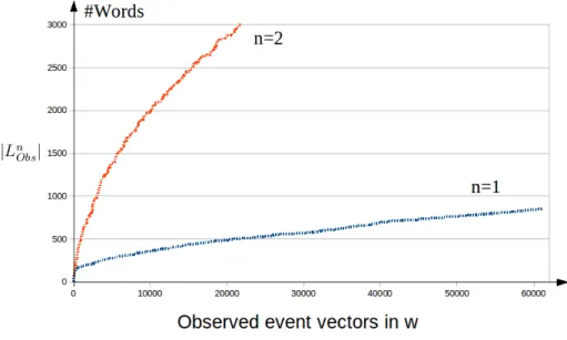
low concurrency, it is possible to observe an asymptote, since the ordering of the output events remains the same during multiple observations of the same processing. On the contrary, highly concurrent systems exhibit lots of possible orderings of events; the number of observed words keeps raising with the duration of observation, as illustrated in Figure1.12.
For low values of n, it is possible to make the assumption that every word that could be emitted by the system was observed, but not for higher values of n. An example of
Figure 1.12: [Roth et al., 2009a] Evolution of the number of observed words of length n over production cycles h
a real system (described in [Roth, 2010]) whose convergence is valid only for n = 1 over a hundred production cycles is presented in Figure 1.13.
Figure 1.13: [Roth, 2010] Observed languages over a hundred production cycles Reasonably, the hypothesis is therefore made that the observation, being finite, is always incomplete. The belonging of a non-observed word to the original language of the system is undecidable. Therefore, no counter-examples can be used in the context of identification of real systems. This caracteristic is highly important, as some related works are based instead on the design and use of counter-examples ([Giua and Seatzu, 2005][Cabasino et al., 2015]). The authors of [Basile et al., 2016c] notably propose to compute timed counter-examples from observed timed sequences, assuming that lower and upper bounds of execution times are known; they are however unavailable in our blackbox approach.
1.2.3 Problem Statement
The following constraints and hypotheses on the systems of interest have been ex-hibited in the previous section:
• Logical input and output signals
• Multiple input-output change between two observations • Inputs might have delayed actions on outputs
• The couple controller/process is non deterministic • The system can exhibit massive concurrency • The identification is blackbox, and passive • No knowledge of counter-examples
We wish to build, from a vector sequence w observed under the above conditions, a model that non only reproduces w, but also exhibits the reactive behaviour of the system in its structure. The main problem of this thesis is stated:
Problem Statement Consider a logical closed-loop system controlled by a PLC.
Identify, from an observed vector sequence w, a model that exhibits the reactive behaviour and reproduces w.
In this problem, no explicit representation of time is required in the model; timed phenomena are present, but the identification of time bounds and their explicit addition in the model are not required. Cyclicity is not required as well; observations do not require to start and end at the same point.
An additional objective is to get an understandable, compact behavioural model, to satisfy a goal of reverse engineering as presented in next section.
1.2.4 Identification for reverse engineering
Reverse engineering is defined in [Chikofsky and Cross II, 1990] as the process of an-alyzing a subject system to identify the systems components and their interrelationships and create representations of the system in another form or at a higher level of abstrac-tion. Identification is a natural method to obtain these representations of the system. Instead of formulating theoretical models, they are constructed from the observation of the real system in its environment.
Potential applications are certification, reimplementation, or debug. In the latter case, an example is [Prähofer et al., 2013], where the authors are interested in the reverse engineering of the program of the PLC. The behaviour called reactive in this article is a change of the path followed by the program depending on the inputs values. The idea is to obtain a model of the paths followed, for analysis and visualization.
For a reactive DES, a good reverse-engineered model should provide insight on the characteristics of the system, such as concurrency, non-determinism or input/output causalities. These caracteristics should be readable in the model, and easily understand-able by an engineer. Readunderstand-able models will facilitate the job of program certification, or reimplementation in a controller.
The choice of the model class should therefore be conditionned by the purpose de-served by the model. Hence, the upcoming literature review exhibitis different methods and models, and discusses their adequation to reverse-engineering. The choice of IPNs as a satisfying model class ensues from this review.
1.3
Identification in the literature
1.3.1 Origin: early computer science approaches
1.3.1.1 Language inference
The problem of DES identification can be retraced to the 60s, and the beginning of artificial intelligence, that motivated the study of language identification [Gold, 1967], also called language inference [Angluin, 1982]. An accurate history is presented in these two surveys on identification: [Estrada-Vargas et al., 2010] and [Cabasino et al., 2015]. The idea of [Gold, 1967] is to present information, as a set of strings s1, s2, . . . ,
to a learner which has to guess the language L; this is quite similar to the observation obtained from a DES (as event generator), where the identification algorithm plays the role of learner. The language L is said identifiable in the limit, if after some time, the learner always guesses the correct language. Two ways of presenting information are considered: either a text containing every string from L (hypothesis of full knowledge of the language), or an informant, which has absolute knowledge on the membership of strings si to L.
This notion of informant, oracle, or teacher was explored in [Angluin, 1987], where the learner can submit queries to the teacher, which can also exhibit counter-examples (strings not belonging to the language). The learning algorithm L∗ proposed is able to
build a deterministic finite-state acceptor (i.e. a DFA) from the information given by the teacher. Full knowledge of the language is a recurrent characteristic of language inference methods, which is not accessible in the case of DES identification.
Angluin’s L∗ algorithm is still used in recent works in the field of computer science,
such as [Shahbaz and Groz, 2009], where the complexity of the processing of counterex-amples is reduced.
1.3.1.2 Moore and Mealy machines
Other methods have focused on the inference of Moore or Mealy machines from input/output sequences.
event sequence of length n: (i1, o1)(i2, o2). . . (in, on). The problem is then to find all
possible reduced machines by state merging operations. The resulting machines are not ’completely specified’, in that they exhibit exceeding behaviour.
[Gill, 1966], then [Heun and Vairavan, 1976] have invested required properties of a set of finite input/output strings in order to be realizable by Mealy machines. [Gill, 1966] characterizes compatibility, extended by [Heun and Vairavan, 1976] into consistency. An algorithm constructing the Mealy machine is provided as well.
In [Biermann, 1972], the maximal number of states of the Mealy machine to be identified is set. The input/output pairs of the sequence are incrementally dealt with, and guesses consistent with the sequence are made on the structure. If no machine can reproduce the behaviour, the procedure is repeated with an increased number of states. Consequently, the final solution has the fewer states of all machines whose behaviour comprises the sample set (i.e. is minimal).
The same author has also investigated non deterministic Moore machines in [ Bier-mann and Feldman, 1972]. A set of i/o sequences is given, where the output is only emitted with the last symbol of the sequence; these sequences are assumed to start from the same initial state. An initial machine is contructed as a tree, then reduced by state merging rules.
Finally, [Veelenturf, 1978] has proposed an iterative algorithm to successively build Mealy machines from a set of observed input/output sequences, such that the behaviour of each machine is included in the result of the previous iteration. New machines are built by adding transition and/or states to the previous one. The sequences are always treated as a whole, contrary to [Biermann, 1972] that deals incrementally with input/output pairs.
The same author has proposed a learning algorithm to identify a Moore machine in [Veelenturf, 1981]. The algorithm guesses structural properties, detects eventual contradictions with the observed i/o sequences, and corrects by removing transition. The inferred automata is minimal.
In all these methods, the notion of input/output is not exploited; the couple (ik, ok)
is interpreted as a symbol. Namely, all the algorithms discovering Mealy machines could be applied on problems without interpretation; they are not specific to represent reactive behaviour.
After this short historical tour, recent approaches in the field of Discrete Event Systems are presented.
1.3.2 Identification by Automata
1.3.2.1 Identification of closed-loop processes
These approaches consider systems close to the ones presented in Section 1.2.1. A whitebox approach for PLC-controlled processes is presented in [Prähofer et al., 2014]. An observation consists in recording the inputs, outputs and taking snapshots of
the program state, from which the path followed by the program in a functional block in a given cycle is deduced (Figure 1.14). Knowledge of the internal state of the controller is therefore known. An FSM is built from these traces, to which are ultimately added time windows. The FSM is a high-level model, representing paths, but the low-level relations of inputs and outputs are not considered.
Figure 1.14: [Prähofer et al., 2014] Left: A flow chart of a function block of the PLC, with the paths numbered. Right: A trace and its representation as a FSM
Identification of PLC-controlled processes have been considered in a series of works. [Klein, 2005][Roth, 2010][Schneider et al., 2012]. The methods proposed in these works have been conceived for fault diagnosis applications. In [Klein, 2005], the identified mod-els are Non Deterministic Autonomous Automata with Outputs (NDAAO). Formally:
Definition 1.18 ([Klein, 2005]NDAAO). A non-deterministic autonomous automaton
with output, is a five-tuple NDAAO = (X, Ω, fnd, λ, x0) where X is the finite set of
states, Ω is the finite set of output symbols, fnd : X → 2X is the non-deterministic
transition relation, x0 ∈ X is the initial state, and Λ : X → Ω is the output function.
In the proposed identification approach, the closed-loop system is considered as an event generator; the choice has been made to build a model that can spontaneously generate events as well. The transition relation is not conditionned by events, hence the autonomy of the model. When a state is reached after a firing, an element of the output alphabet is emitted (as in a Moore machine). Since the observation of the system consists in vectors w(k) (see Section1.2.1), each different observed vector is mapped to an output symbol. Thus, the model can generate output sequences homogeneous to the observed vectors.
An example of the identification procedure is given below, for a plant with two inputs and one output. Notice that the observed sequences start and end with the same vector, which assumes cyclicity of the process observed, an hypothesis not made in our problem.
![Figure 1.22: [Van der Aalst et al., 2004] The net mined by the α -algorithm from the log {ABCD, ACBD, AED}](https://thumb-eu.123doks.com/thumbv2/123doknet/14583261.729562/54.893.212.717.120.310/figure-van-aalst-mined-algorithm-abcd-acbd-aed.webp)