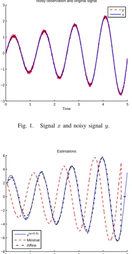
Non-asymptotic fractional order differentiators via an algebraic parametric method

This paper addresses the reliable synchronization problem between two non-identical chaotic fractional order systems. In this work, we present an adap- tive feedback control scheme

A recent study [14] introduced a hybrid spectral method for quantifying the uncertainties in single input single output (SISO) fractional order systems.. This paper extends

The proposed identi?cation method is based on the recursive least squares algorithm applied to an ARX structure derived from the linear fractional order differential equation

The proposed identification method is based on the recursive least squares algorithm applied to a linear regression equation derived from the linear fractional order

The proposed identification technique is based on the recursive least squares algorithm applied to a linear regression equation using adjustable fractional order differentiator

Based on the estimation of the lateral dynamics with the observer proposed in [1], a second estimator is presented in this paper to reconstruct the longitudinal tire-road forces,

Section 5 com- pares the numerical results in image denoising with the Bai and Feng’s algorithm, and some denoising and inpainting ap- plications are performed and compared with

We briefly discuss the issue of controlling fractional-order chaotic Chen, R¨ ossler and modified Chua systems to realize synchronization with linear error feedback con- trol. For