The Green-Kubo formula and the Onsager reciprocity relations in quantum statistical mechanics

HAL Id: hal-00005386

https://hal.archives-ouvertes.fr/hal-00005386

Submitted on 15 Jun 2005

HAL is a multi-disciplinary open access

archive for the deposit and dissemination of

sci-entific research documents, whether they are

pub-lished or not. The documents may come from

teaching and research institutions in France or

abroad, or from public or private research centers.

L’archive ouverte pluridisciplinaire HAL, est

destinée au dépôt et à la diffusion de documents

scientifiques de niveau recherche, publiés ou non,

émanant des établissements d’enseignement et de

recherche français ou étrangers, des laboratoires

publics ou privés.

relations in quantum statistical mechanics

Vojkan Jaksic, Yoshiko Ogata, Claude-Alain Pillet

To cite this version:

Vojkan Jaksic, Yoshiko Ogata, Claude-Alain Pillet.

The Green-Kubo formula and the Onsager

reciprocity relations in quantum statistical mechanics. Communications in Mathematical Physics,

Springer Verlag, 2006, 265 (3), pp.721-738. �10.1007/s00220-006-0004-6�. �hal-00005386�

relations in quantum statistical mechanics

V. Jakši´c

, Y. Ogata

,3

, C.-A. Pillet

Department of Mathematics and Statistics

McGill University

805 Sherbrooke Street West

Montreal, QC, H3A 2K6, Canada

2

CPT-CNRS, UMR 6207

Université du Sud, Toulon-Var, B.P. 20132

F-83957 La Garde Cedex, France

Department of Mathematical Sciences

University of Tokyo

Komaba,Tokyo,153-8914 Japan

June 15, 2005

Dedicated to David Ruelle on the occasion of his 70th birthday

Abstract

We study linear response theory in the general framework of algebraic quantum statistical mechanics and prove the Green-Kubo formula and the Onsager reciprocity relations for heat fluxes generated by temperature differentials. Our derivation is axiomatic and the key assumptions concern ergodic properties of non-equilibrium steady states.

1

Introduction

This is the first in a series of papers dealing with linear response theory in non-equilibrium quantum statistical mechanics. The three pillars of linear response theory are the Green-Kubo formula (GKF), the Onsager reciprocity relations (ORR), and the Central Limit Theorem. This paper and its sequels [JOP1, JOP2] deal with the first two. An introduction to linear response theory in the algebraic formalism of quantum statistical mechanics can be found in the recent lecture notes [AJPP1]. We emphasize that our program is concerned with purely thermodynamical (i.e. "non-mechanical") driving forces such as deviations of temperature and chemical potential from their equilibrium values.

The main result of this paper is an abstract derivation of the GKF and the ORR for heat fluxes. Various gener-alizations of our model and results (and in particular, the extension of GKF and ORR to heat and charge fluxes) are discussed in [JOP1]. Our abstract derivation directly applies to open quantum systems with free fermionic reser-voirs previously studied in [Da, LeSp, BM, AM, JP2, FMU]. These applications are discussed in [JOP2, JOPP].

The mathematical theory of non-equilibrium quantum statistical mechanics has developed rapidly over the last several years. The key notions of non-equilibrium steady states (NESS) and entropy production have been introduced in [Ru1, Ru2, Ru3, JP1, JP2, JP3]. The general theory has been complemented with the development of concrete techniques for the study of non-equilibrium steady states [Ru1, JP2, FMU] and at the moment there are several classes of non-trivial models whose non-equilibrium thermodynamics is reasonably well-understood. The development of linear response theory is the natural next step in this program.

The GKF for mechanical perturbations has been studied in many places in the literature (see [BGKS, GVV1] for references and additional information). Mathematically rigorous results for thermodynamical perturbations are much more scarce. Our research has been partly motivated by the work of Lebowitz and Spohn [LeSp] who studied linear response theory for quantum Markovian semigroups describing dynamics of open quantum systems in the van Hove weak coupling limit. The ORR for directly coupled fermionic reservoirs have been discussed in [FMU] in first order of perturbation theory. The mean field theory aspects of ORR are discussed in [GVV2]. A fluctuation theorem related to linear response theory can be found in [TM]. Needless to say, physical aspects of linear response theory are discussed in many places in the literature, and in particular in the classical references [DGM, KTH]. An exposition in spirit close to our approach can be found in [Br, Zu, ZMR1, ZMR2]. Linear response theory in classical non-equilibrium statistical mechanics has been reviewed in [Ru4, RB].

Our model can be schematically described as follows. Consider two infinitely extended quantum systems which for convenience we will call the left,L, and the right, R, system. The systems L and R may have additional

structure (for example, in the case of open quantum systemsL will consists of a "small" (finite level) system S

coupled to several reservoirs andR will be another reservoir coupled to the small system, see Figure 1).

Assume that initially the systemL is in thermal equilibrium at a fixed (reference or equilibrium) inverse

tem-perature βL= β, and that the system R is in thermal equilibrium at inverse temperature βR. The thermodynamical force X is equal to the deviation of the inverse temperature of the right system from the equilibrium value β,

X= β − βR.

Assume that the systemsL and R are brought into contact. One expects that under normal conditions the joint

systemL + R will rapidly settle into a steady state ωX,+. If X = 0, then ω0,+ ≡ ωβ is the joint thermal equilibrium state ofL + R characterized by the Kubo-Martin-Schwinger (KMS) condition. If X 6= 0, then ωX,+ is a non-equilibrium steady state (NESS) characterized by non-vanishing entropy production

Ep(ωX,+) = XωX,+(Φ) > 0,

whereΦ is the observable describing the heat flux out of R. For additional information about this setup we refer

the reader to [Ru1, Ru2, Ru3, JP1, JP2, JP3].

The Green-Kubo linear response formula asserts that if the joint system is time-reversal invariant and the observable A is odd under time-reversal, then

∂XωX,+(A)¯¯_X=0= 1 2 Z ∞ −∞ ωβ(AΦt)dt, (1.1)

S

Φ

L

β

=

β

− X

β

=

β

R

Figure 1: An open quantum system represented asL + R.

where t7→ Φtis the dynamics in the Heisenberg picture. This celebrated formula relates the linear response to the equilibrium correlations and is a mathematical expression of the fluctuation-dissipation mechanism in statistical mechanics.

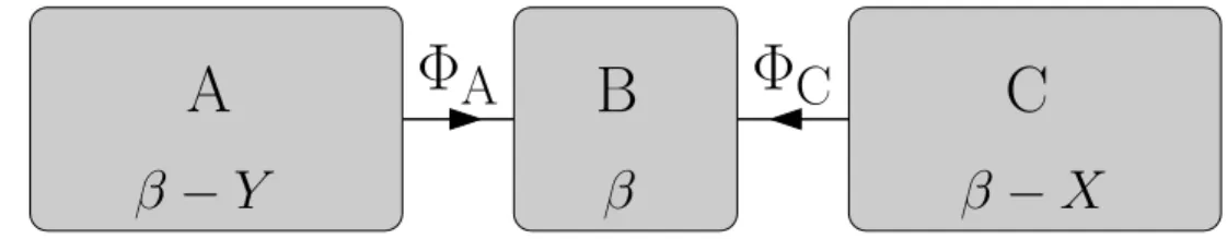
The ORR are direct consequences of the GKF. Consider three systems A, B, C, which are respectively in

thermal equilibrium at inverse temperatures β − Y , β, and β − X. Assume that the systems are brought into

contact by interactions which coupleA with B and B with C. Let ωX,Y,+be the non-equilibrium steady state of the joint system andΦA,ΦCthe observable which describe the heat flow out ofA, C (see Figure 2). If the system is time-reversal invariant, thenΦAandΦCare odd under time-reversal.

Assume that the functions ωX,Y,+(ΦC) and ωX,Y,+(ΦA) are differentiable at X = Y = 0. The kinetic transport coefficients are defined by

LA≡ ∂XωX,Y,+(ΦA)¯¯_{X=Y =0}, LC≡ ∂YωX,Y,+(ΦC)

¯ ¯_{X=Y =0}.

In words, even ifA and B are at the same temperature, the temperature differential between B and C may cause

a heat flux out ofA equal to XLA+ o(X) for X small. LChas the same interpretation. If the GKF in the form (1.1) holds forL = A + B, R = C and A = ΦA, then

LA=1

2 Z ∞

−∞

ωβ(ΦA(ΦC)t)dt. Similarly, if the GKF holds forL = B + C, R = A and A = ΦC, then

LC= 1 2 Z ∞ −∞ ωβ(ΦC(ΦA)t)dt = 1 2 Z ∞ −∞ ωβ((ΦC)tΦA)dt. Hence, the GKF and the relation

Z ∞

−∞

ωβ([(ΦC)t,ΦA])dt = 0,

which is a well-known consequence of the KMS condition, yield the Onsager reciprocity relations

LA= LC. (1.2)

In this paper we give a rigorous axiomatic proof of the GKF (1.1) and the ORR (1.2) in the abstract setting of algebraic quantum statistical mechanics.

The main idea of our proof can be illustrated by the following simple computation. Assume that L and R

are finite dimensional systems, i.e., that they are described by finite dimensional Hilbert spaces HL, HR and Hamiltonians HL, HR. The Hilbert space of the joint system isH = HL⊗ HR. Let V be a self-adjoint operator

Φ

_C

Φ

_A

A

B

C

β

− X

β

β

− Y

Figure 2: The joint systemA + B + C.

onH describing the interaction of L and R. The Hamiltonian of the joint system is H = HL+ HR+ V and

At= eitHAe−itH. The heat flux observable is

Φ = −d dte itH HRe−itH ¯ ¯ t=0= i[HR, V]. (1.3) A common choice for the reference (initial) state of the joint system is the product state ωrefwith density matrix

1 Ze

−βHL−(β−X)HR

,

where Z is a normalization constant. As we shall see, in the study of linear response theory a more natural choice is the state ωXdescribed by the density matrix

1 Ze

−βH+XHR

.

Let A be an operator onH and t > 0. Note that ωX(At) = ωX

³

e−it(H−XHR/β)_eitH_Ae−itH_eit(H−XHR/β)

´ , and so ωX(At) − ωX(A) = X β Z t 0 ωX(i[HR, As])ds. (1.4) If the system is time-reversal invariant and A is odd under the time-reversal operation, then ωX(A) = 0 for all X (and in particular, ω0(At) = ω0(A) = 0 for all t). Hence, (1.4) yields

∂XωX(At) ¯ ¯_X=0= 1 β Z t 0 ωβ(i[HR, As])ds. Another elementary computation yields

ωβ(i[HR, As]) = i ZTr(As[e −βH_{, H} R]) = i ZTr¡As[e −βH_H ReβH− HR]e−βH¢ = Z β 0

ωβ(Ase−uHΦeuH)du, and so ∂XωX(At) ¯ ¯_X=0= 1 β Z t 0 ds Z β 0 du ωβ(AsΦiu). (1.5) Needless to say, only infinitely extended systems have non-trivial thermodynamics. The central point of our argument is that the relation (1.5) can be proven even if the systemsL and R are infinitely extended and

and holds in the abstract setting of algebraic quantum statistical mechanics under very mild technical conditions. Our argument then continues as follows. Assume that there exists a state ωX,+onO such that for any observable

A,

lim

t→+∞ωX(At) = ωX,+(A). (1.6) The state ωX,+is the non-equilibrium steady state (NESS) of the systemL + R and is the central object of non-equilibrium statistical mechanics. Let A be an observable for which (1.5) holds. Assume in addition that the function

X 7→ ωX,+(A), (1.7)

is differentiable at X = 0 and that the limit and the derivative in the expression lim

t→+∞∂XωX(At)

¯

¯_X=0, (1.8)

can be interchanged. Then,

∂XωX,+(A)¯¯ X=0= 1 β Z ∞ 0 dt Z β 0 du ωβ(AtΦiu), (1.9) and this relation is the Green-Kubo formula.

If in addition the joint thermal equilibrium state ωβis mixing, namely if for all A, B∈ O,

lim

|t|→∞ωβ(τ

t_{(A)B) = ω}

β(A)ωβ(B), (1.10)

then it is not difficult to show that the KMS condition and the time-reversal invariance imply that (1.9) is equivalent to (1.1).

The above derivation requires a comment. The initial state commonly used in the literature is the decoupled product state ωref. In this paper we prove the GKF for the NESS ωX,+associated to the initial state ωX. On physical grounds, one expects that under normal conditions all states normal w.r.t. ωXevolve to ωX,+as t→ +∞ (see [JP3, AJPP1]). Since in particular ωX and ωref are mutually normal they are physically equivalent initial states.

The three key assumptions of our derivation are the existence of the NESS (1.6), the differentiability of the function (1.7), and the interchange of the limit and the derivative in (1.8). Verification of each of them in physically interesting models is a difficult task.

In the literature two distinct techniques have been used so far in the study of NESS. The first is the scattering approach, initiated by Robinson [Ro1], and further developed in [BM, AM, Ru1, FMU]. The second is the spectral approach developed in [JP2]. In the continuation of this paper [JOP2, JOPP] we will show how the spectral and the scattering approach can be used to verify our abstract assumptions and we will illustrate the general theory on well-known examples of open quantum systems with free fermionic reservoirs studied in [Da, LeSp, BM, AM, JP2, FMU].

Acknowledgment. The research of the first author was partly supported by NSERC. Part of this work was done

during the visit of the first and the third author to ESI in Vienna. V.J. and C.-A.P. are grateful to J. Derezi´nski, G.-M. Graf and J. Yngvason for invitation to the workshop "Open Quantum Systems" and for their hospitality. A part of this work has been done during the visit of the first author to CPT-CNRS. Y.O. is supported by the Japan Society for the Promotion of Science. This work has been done during the stay of Y.O. to CPT-CNRS, partly supported by the Canon Foundation in Europe and JSPS.

2

The model and the results

2.1

Basic concepts

In this subsection we briefly review for notational purposes a few basic notions of algebraic quantum statistical mechanics. This topic is discussed in many places in the literature and we will freely use the results described in the classical references [BR1, BR2]. An exposition of the algebraic formalism suited to non-equilibrium quantum statistical mechanics can be found in the reviews [Ru3, JP3, AJPP1].

A C∗-dynamical system is a pair(O, τ ), where O is a C∗_{-algebra with identity1l and τ}t_{, t∈ R, is a strongly} continuous group of ∗-automorphisms of O. In the context of quantum statistical mechanics, the elements of O describe observables of a physical system and the group τ describes their time evolution in the Heisenberg

picture. The physical states are described by the states onO, i.e., positive normalized linear functionals in O∗_{. A} quantum dynamical system is a triple(O, τ, ω), where ω is a given reference state. The physical states of thermal

equilibrium at inverse temperature β are described by (τ, β)-KMS states in O∗_{. We shall assume that β > 0} although all our results also apply to β <0. We recall that ω is a (τ, β)-KMS state if for all A, B ∈ O there exists

a function FA,B(z), analytic in the strip 0 < Im z < β, bounded and continuous on its closure, and satisfying the KMS-boundary condition

FA,B(t) = ω(Aτt(B)), FA,B(t + iβ) = ω(τt(B)A). The three-line theorem yields that

|FA,B(z)| ≤ kAkkBk,

for0 ≤ Im z ≤ β. For notational convenience we shall write ω(Aτz_{(B)) ≡ F} A,B(z). An anti-linear involutive∗-automorphism Θ : O → O is called time-reversal of (O, τ ) if

Θ ◦ τt= τ−t◦ Θ,

for all t∈ R. A state ω is called time-reversal invariant if ω(Θ(A)) = ω(A∗_{) for all A ∈ O.}

2.2

The setup

We shall consider two quantum dynamical systems(OL, τL, ωL) and (OR, τR, ωR), which we shall call the left, L, and the right,R, system. We denote the generators of τLand τRby δLand δR, i.e., τLt= etδ

L_{and τ}t

R= etδ

R_.

If the systemL and R are brought into contact, then the algebra of observables of the joint system is O = OL⊗ OR(our results do not depend on the choice of the cross-norm defining this tensor product). Its decoupled dynamics τ0= τL⊗ τRis generated by δ(0)= δL+ δR.

Notation. IfL is an operator on OL, then we will denote by the same letter the operatorL ⊗ I on OL⊗ OR. Hence, we write δLfor δL⊗ I, etc. We will use the same convention in the case of OR.

Let V ∈ O be a self-adjoint perturbation describing the interaction of L and R. The C∗_{-dynamical system} describing the interacting systemL + R is (O, τ ), where the interacting dynamics τ is generated by

δ= δ(0)+ i[V, ·].

In what follows β >0 is a fixed reference inverse temperature and ² > 0 is a small number such that β > ².

We set I² = (−², ²). We make the following assumptions concerning the reference states of L and R and the interaction V .

(A1) ωL is the unique(τL, β)-KMS state on OL. The possible reference states ofR are parametrized by X ∈ I² and ωR,Xis the unique(τR, β− X)-KMS state on OR. We shall write ωR,0= ωR.

(A2) V ∈ Dom (δR).

If (A2) holds, then the observable describing the heat flux out ofR is (recall (1.3)) Φ ≡ δR(V ).

Consider the family of states

ω_X(0)= ωL⊗ ωR,X. Let σ_X(0)and σXbe the C∗-dynamics onO generated by

δ(0)_X = δ(0)−X βδR, δX= δ(0)X + i[V, ·].

ω_X(0) is the unique(σ(0)_X , β)-KMS state on O. The Araki perturbation theory implies that there exists a unique (σX, β)-KMS state ωX onO. The states ωX and ωX(0)are mutually normal. Note that σ0 = τ and that ω0is the unique(τ, β)-KMS state on O. We denote ωβ≡ ω0.

Our next assumption deals with time-reversal invariance.

(A3) There exists a time-reversalΘ of (O, τ0) such that

Θ ◦ τt L= τ −t L ◦ Θ, Θ ◦ τRt = τ −t R ◦ Θ, Θ(V ) = V.

One easily shows thatΘ is also a time-reversal of (O, τ ), (O, σ_X(0)) and (O, σX). If in addition (A1) holds, then the states ω_X(0)and ωXare time-reversal invariant.

In essence, our main result is:

Theorem 2.1 Suppose that Assumptions (A1)-(A3) hold. Let A ∈ Dom (δR) be a self-adjoint observable such thatΘ(A) = −A. Then, for all t ∈ R, the function

X 7→ ωX(τt(A)), is differentiable at X= 0, and ∂XωX(τt(A)) ¯ ¯_X=0= 1 β Z t 0 ds Z β 0 du ωβ(τs(A)τiu(Φ)). (2.11)

Remark 1. Assume in addition that the quantum dynamical systems(OR, τR, ωR,X) are ergodic for |X| < ². Then, {ωX} is a family of mutually singular states (see [JP3, AJPP1]) and the differentiability of the function

X 7→ ωX(τt(A)) at X = 0 is far from obvious. The somewhat surprising generality of Theorem 2.1 critically depends on the time-reversal assumption which ensures that ωX(A) = 0 for all |X| < ². For a related technical point in classical non-equilibrium statistical mechanics we refer the reader to [Ru5].

Remark 2. Let ωβ,λdenote the β-KMS state for the C∗-dynamics generated by δ− λ[Ξt,· ] where

Ξt≡

Z t

0

τ−s(Φ)ds.

Then, by Araki’s perturbation theory one has

1

β∂λωβ,λ(A) ¯

¯_λ=0= ∂XωX(τt(A))¯¯_X=0.

Hence, the finite time t linear response to the thermodynamical force X is equal, up to a factor of β, to the equilibrium linear response to the mechanical perturbationΞt. For additional information concerning this point we refer the reader to [Zu, TM].

2.3

The Green-Kubo formula

Our next assumption postulates the existence of a NESS w.r.t. the initial state ωX.

(A4) For each X∈ I²there exists a state ωX,+such that for all A∈ O,

lim

t→+∞ωX(τ

t_{(A)) = ω} X,+(A). Note that ω0,+= ωβis the unique(τ, β)-KMS state on O.

Finally, we shall assume that our coupled system is mixing at equilibrium.

(A5) For all A, B∈ O,

lim

|t|→∞ωβ(τ

t_{(A)B) = ω}

β(A)ωβ(B).

The observables for which we will establish the Green-Kubo formula are characterized by

Definition 2.2 Assume that (A1) and (A4) hold. Let A∈ O be an observable such that for all t the function X 7→ ωX(τt(A)),

is differentiable at X= 0. We call such an observable regular if the function

X 7→ ωX,+(A), (2.12) is differentiable at X= 0 and lim t→+∞∂XωX(τ t_(A))¯ ¯_X=0= ∂XωX,+(A)¯¯_X=0. (2.13)

A consequence of Theorem 2.1 and the definition of regular observable is the Green-Kubo formula.

Theorem 2.3 Suppose that Assumptions (A1)-(A4) hold. Let A∈ Dom (δR) be a regular self-adjoint observable such thatΘ(A) = −A. Then

∂XωX,+(A) ¯ ¯_X=0= 1 β Z ∞ 0 dt Z β 0 du ωβ(τt(A)τiu(Φ)). (2.14) If in addition (A5) holds, then

∂XωX,+(A)¯¯_X=0= 1 2 Z ∞ −∞ dt ωβ(Aτt(Φ)). (2.15) Remark 1. In (2.15),R∞ −∞= limT →∞ RT −T.

Remark 2. It follows from our proof that linear response to the thermodynamical force X can be computed without

time-reversal assumption. Assume that (A1), (A2), (A4) hold and that A∈ Dom (δR) is a regular observable. Then

∂XωX,+(A)¯¯ X=0= ∂XωX(A) ¯ ¯ X=0+ 1 β Z ∞ 0 dt Z β 0 du ωβ(τt(A)τiu(Φ)). This formula will be discussed in more detail in [JOP1].

In applications to concrete models the key assumptions to check are (A4), (A5) and that physically relevant observables are regular. The assumptions (A4) and (A5) have been verified for open quantum systems with free Fermi gas reservoirs in [BM, AM, JP2, FMU]. In these works (A4) is established in the stronger form, i.e. for any η normal w.r.t. ω_X(0)and all A∈ O, limt→+∞η(τt(A)) = ωX,+(A). In the continuation of this paper [JOP2, JOPP] we will prove that in these models the observables describing heat fluxes withinL are regular.

A simple class of models to which Theorem 2.3 directly applies are quasi-free open systems studied in [AH, AJPP1, AJPP2, AP]. These models are also exactly solvable and the GKF and the ORR can be checked by direct computation.

2.4

Onsager reciprocity relations

Consider three C∗-dynamical systems(OJ, τJ), J = A, B, C. The generator of τJis denoted by δJ. We set

O =O J OJ, τ0= O J τJ, δ(0)= X J δJ.

Let V ∈ O be a self-adjoint perturbation describing the interaction of the joint system and let τ be the dynamics

generated by δ= δ(0)_{+ i[V, ·]. We shall assume that V has the form}

V = VAB+ VBC,

where VAB ∈ OA⊗ OBand VBC∈ OB⊗ OC. If VAB ∈ Dom (δA) and VBC∈ Dom (δC), then the observables describing the heat flow out of A and C are

ΦA= δA(VAB), ΦC= δC(VBC), see Figure 2. Note that in this case δC(ΦA) = δA(ΦC) = 0.

We assume that (A3) holds in the following form: there exists a time-reversalΘ of (O, τ0) such that τJt◦ Θ =

Θ ◦ τ_J−tfor all J andΘ(VAB) = VAB,Θ(VBC) = VBC. ThenΘ is a time-reversal of the coupled system (O, τ ) andΘ(ΦA) = −ΦA,Θ(ΦC) = −ΦC.

We shall also consider the joint systems A + B and B + C. In the first case the algebra of observables is OA⊗ OB and the dynamics is generated by δA+ δB+ i[VAB,·]. The system B + C is defined in a similar way. Let β >0 be the fixed inverse temperature.

ConsiderL = A + B as the left system and R = C as the right system. Suppose that Assumptions (A1), (A2),

(A4), (A5) hold (we have already assumed the time-reversal invariance) and that the observableΦAis regular. Let

ωA+B,C,X,+be the NESS in the Assumption (A4). Then the kinetic transport coefficient

LA= ∂XωA+B,C,X,+(ΦA)

¯ ¯

X=0, is well-defined and the Green-Kubo formula holds,

LA= 1 2 Z ∞ −∞ ωβ(ΦAτt(ΦC))dt, where ωβis the(τ, β)-KMS state on O.

Consider nowL = B + C as the left system and R = A as the right system. Suppose that Assumptions (A1),

(A2), (A4) and (A5) hold and that the observableΦCis regular. Let ωB+C,A,X,+be the NESS in the Assumption (A4). Then the kinetic transport coefficient

LC= ∂XωB+C,X,+(ΦC)

¯ ¯_X=0,

is well-defined and the Green-Kubo formula holds,

LC= 1 2 Z ∞ −∞ ωβ(ΦCτt(ΦA))dt = 1 2 Z ∞ −∞ ωβ(τt(ΦC)ΦA)dt.

Since ωβis mixing, by the well-known stability criterion (Theorem 5.4.12 in [BR2]), lim T →∞ Z T −T ωβ([τt(ΦC), ΦA])dt = 0, and so LA= LC. This is the Onsager reciprocity relations for heat fluxes.

3

Proofs

Throughout this subsection we assume that (A1) and (A2) hold. We start with:

Lemma 3.1 Assume that(A3) holds. Then:

(1)Θ is a time-reversal of the C∗-dynamical systems(O, τ ) and (O, σX), (2) The states ωXare time-reversal invariant.

(3)Θ(Φ) = −Φ.

Proof. (1) Recall that

τt(A) = Γtτ0t(A)Γ∗t, (3.16) whereΓt∈ O is the family of unitary elements defined by

Γt= 1l + X n≥1 (it)n Z 0≤sn≤···≤s1≤1 τtsn 0 (V ) · · · τts 1 0 (V )ds1· · · dsn, (3.17) see Proposition 5.4.1. in [BR2]. Similarly,

τ−t(A) = ˆΓtτ0−t(A)ˆΓ∗t, where ˆ Γt= 1l + X n≥1 (−it)n Z 0≤sn≤···≤s1≤1 τ−tsn 0 (V ) · · · τ −ts1 0 (V )ds1· · · dsn.

SinceΘ(V ) = V and Θ(Γt) = ˆΓt, we have thatΘ ◦ τt= τ−t◦ Θ, i.e., Θ is a time-reversal of (O, τ ).

SinceΘ is also a time-reversal of (O, σX(0)), one proves in the same way that Θ is a time-reversal of (O, σX). (2) Set

˜

ωX(A) = ωX(Θ(A∗)).

One easily checks thatω˜X is a(σX, β)-KMS state. Assumption (A1) and Araki’s perturbation theory imply that

ωXis the unique(σX, β)-KMS state on O. Hence, ˜ωX = ωX. (3) is an immediate consequence of the relationΘ(τt

R(V )) = τ −t

R (V ) and the definition of Φ. 2

Lemma 3.2 The group τ preservesDom (δR) and for A ∈ Dom (δR) the function

R_{3 t 7→ δR(τ}t_(A)),

Proof. Since V ∈ Dom (δR), the formula (3.17) yields that Γt∈ Dom (δR) and that δR(Γt) = X n≥1 (it)n Z 0≤sn≤···≤s1≤1 X j τtsn 0 (V ) · · · τ tsj 0 (δR(V )) · · · τ0ts1(V )ds1· · · dsn.

The series on the right is uniformly convergent for t in compact sets, and so R3 t 7→ δR(Γt) is a norm continuous function. The formula (3.16) yields

δR(τt(A)) = δR(Γt)τ0t(A)Γ∗t+ Γtτ0t(δR(A))Γ∗t+ Γtτ0t(A)δR(Γt)∗, and the statement follows. 2

In the remaining part of the proof we will need to approximate A and V by analytic elements. For this reason we briefly recall a few basic facts about such analytic approximations (see [Ar, BR2, DJP]). For C∈ O we set

Cj= r j π Z R e−jt2τ₀t(C)dt, j= 1, 2, · · · (3.18) Every Cj is an analytic element for the group τ0, i.e., the function t7→ τ0t(Cj) ∈ O extends to an entire analytic function on C. Moreover,

kCjk ≤ kCk and lim

j→∞kCj− Ck = 0. (3.19) If in addition C ∈ Dom (δR), then

δR(Cj) = r j π Z R e−jt2τ₀t(δR(C))dt, j = 1, 2, · · · and so δR(Cj) is also an analytic element for τ0tandlimj→∞kδR(Cj) − δR(C)k = 0.

Lemma 3.3 For A∈ Dom (δR),

σXt (A) − τt(A) = − X β Z t 0 σt−s_X (δR(τs(A)))ds. (3.20)

Proof. Assume first that A∈ Dom (δ) ∩ Dom (δR). Then,

d dtσ −t X(τ t_{(A)) = σ}−t X((δ − δX)(τ t_{(A))) =} X β σ −t X(δR(τ t_{(A))), (3.21)} and (3.20) holds.

Let now A∈ Dom (δR) and let Aj be given by (3.18). Clearly, Aj ∈ Dom (δ) ∩ Dom (δR) and (3.20) holds for Aj. The relations

δR(τt(Aj)) = δR(Γtτ0t(Aj)Γ∗t)

= δR(Γt)τ0t(Aj)Γ∗t+ Γtτ0t(δR(Aj))Γ∗t+ Γtτ0t(Aj)δR(Γt)∗,

yield thatlimj→∞δR(τt(Aj)) = δR(τt(A)) uniformly for t in compact sets, and the statement follows. 2 SinceDom (δR) is dense in O, Lemma 3.3 yields that for all A ∈ O,

lim

X→0kσ t

Lemma 3.4 For all A∈ O,

lim

X→0ωX(A) = ωβ(A).

Proof. LetL be the set of weak* limit points of the net {ωX} as X → 0. The set L is non-empty since the unit ball inO∗_{is weak* compact. Relation (3.22) and Proposition 5.3.25 in [BR2] yield that every element ofL is a}

(τ, β)-KMS state. Assumption (A1) implies that ωβis the unique(τ, β)-KMS state on O and so L = {ωβ}. 2

Lemma 3.5 Assume that (A3) holds. Let A ∈ Dom (δR) be a self-adjoint observable such that Θ(A) = −A. Then for all t∈ R the function

X 7→ ωX(τt(A)), is differentiable at X= 0 and ∂XωX(τt(A)) ¯ ¯_X=0= 1 β Z t 0 ωβ(δR(τs(A)))ds.

Proof. Since ωXis σX-invariant, Lemma 3.3 yields

ωX(τt(A)) − ωX(A) X = 1 β Z t 0 ωX(δR(τs(A)))ds.

By Lemma 3.1, ωX(A) = ωX(Θ(A)) = −ωX(A), and so ωX(A) = 0. Similarly, since ω0 = ωβis τ -invariant,

ω0(τt(A)) = ω0(A) = 0 for all t. Hence,

ωX(τt(A)) − ω0(τt(A)) X = 1 β Z t 0 ωX(δR(τs(A)))ds. This relation, Lemmas 3.2, 3.4, and the dominated convergence yield the statement. 2

Lemma 3.6 Assume that A∈ Dom (δR). Then

ωβ(δR(A)) =

Z β

0

ωβ(Aτis(Φ))ds.

Proof. We will freely use standard results of Araki’s theory of perturbation of KMS-states (see [Ar, BR2, DJP]).

Let Vj be the analytic approximations of V given by (3.18). Since V ∈ Dom (δR), Φj ≡ δR(Vj) are analytic approximations of the heat flux observableΦ = δR(V ). Note also that the function t 7→ Γt,j, where

Γt,j= 1l + X n≥1 (it)n Z 0≤sn≤···≤s1≤1 τtsn 0 (Vj) · · · τ0ts1(Vj)ds1· · · dsn, extends to an entire analyticO-valued function

Γz,j= 1l + X n≥1 (iz)n Z 0≤sn≤···≤s1≤1 τzsn 0 (Vj) · · · τ0zs1(Vj)ds1· · · dsn. The function z7→ Γ∗

Let τjbe the C∗-dynamics onO generated by δ(0)+ i[Vj,·], and let ωjbe the unique(τj, β)-KMS state. Since for any C∈ O,

τjt(C) = Γt,jτ0t(C)Γ∗t,j, (3.23) we conclude that Aj, Vj, andΦjare also analytic elements for τjand thatlimj→∞kτjt− τ k = 0.

We shall prove first that for all j,

ωj(δR(Aj)) =

Z β

0

ωj(Ajτjiu(Φj))du. (3.24) This formula combined with a limiting argument j→ ∞ will yield the statement.

The following relations hold

d dzΓz,j= iΓz,jτ z 0(Vj), d dzΓ ∗ z,j= −iτ0z(Vj)Γ∗z,j. (3.25)

One easily verifies that for all z ∈ C, Γz,j ∈ Dom (δR), Γ∗z,j ∈ Dom (δR), that the functions z 7→ δR(Γz,j),

z7→ δR(Γ∗z,j) are entire analytic, and that

d dzδR(Γz,j) = iδR(Γz,j)τ z 0(Vj) + iΓz,jτ0z(Φj), d dzδR(Γ ∗ z,j) = −iτ0z(Φj)Γ∗z,j− iτ0z(Vj)δR(Γ∗z,j). (3.26)

Relations (3.25) and (3.26) yield

d

dzΓz,jδR(Γ

∗

z,j) = −iΓz,jτ0z(Φj)Γ∗z,j= −iτjz(Φj). (3.27) Recall that ω(0)₀ = ωL⊗ ωR. By the basic identity of Araki’s perturbation theory, for any C∈ O,

ωj(C) = ω₀(0)(CΓiβ,j) ω₀(0)(Γiβ,j) . In particular, ωj(δR(Aj)) = ω₀(0)(δR(Aj)Γiβ,j) ω(0)₀ (Γiβ,j) .

Since ω₀(0)(δR(C)) = 0 for any C ∈ Dom (δR), we have

ω0(0)(δR(Aj)Γiβ,j) = −ω0(0)(AjδR(Γiβ,j)) = −ω(0)0 (Aj[δR(Γiβ,j)Γ∗−iβ,j]Γiβ,j). Hence, ωj(δR(Aj)) = ωj(Aj[Γiβ,jδR(Γ∗−iβ,j)]). (3.28) Relation (3.27) implies d duΓiu,jδR(Γ ∗ −iu,j) = τjiu(Φj),

and so

Γiβ,jδR(Γ∗−iβ,j) =

Z β

0

τ_jiu(Φj)du. (3.29)

Relations (3.28) and (3.29) yield (3.24). It remains to show that

lim j→∞ωj(δR(Aj)) = ωβ(δR(A)), (3.30) lim j→∞ Z β 0 ωj(Ajτjiu(Φj))du = Z β 0 ωβ(Aτiu(Φ))du. (3.31) By the properties of analytic approximations,

lim

j→∞kωj− ωβk = 0 and j→∞lim kδR(Aj) − δR(A)k = 0, and these relations yield (3.30). To prove (3.31) we argue as follows.

For t∈ R we set hj(t) = Z β 0 ωj(Ajτjiu+t(Φj))du, h(t) = Z β 0

ωβ(Aτiu+t(Φ))du. Then Z t 0 ωj([Aj, τju(Φj)])du = Z t 0 ωj(Ajτju(Φj))du − Z t 0 ωj(Ajτju+iβ(Φj))du = i Z β 0 ωj(Ajτjiu(Φj))du − i Z β 0 ωj(Ajτjiu+t(Φj))du = i(hj(0) − hj(t)).

In the first step we have used the KMS condition and in the second that the integral of the function z 7→ ωj(Ajτjz(Φj)) over the boundary of the rectangle with vertices 0, t, t + iβ, iβ is zero. Similarly,

Z t

0

ωβ([A, τu(Φ)])du = i(h(0) − h(t)). Since

lim

j→∞ωj([Aj, τ u

j(Φj)]) = ωβ([A, τu(Φ)]), we derive that for all t∈ R

lim j→∞(hj(t) − hj(0)) = h(t) − h(0). (3.32) Note that Z ∞ −∞ e−t2hj(t)dt = Z β 0 du Z ∞ −∞ dt e−(t−iu)2ωj(Ajτjt(Φj)), Z ∞ −∞ e−t2h(t)dt = Z β 0 du Z ∞ −∞ dt e−(t−iu)2ωβ(Aτt(Φ)). Since for all t,

lim

j→∞ωj(Aτ t

we conclude that lim j→∞ Z ∞ −∞ e−t2(hj(t) − h(t))dt = 0. (3.33) Then (3.32) and (3.33) yield

lim

j→∞hj(0) = h(0), and (3.31) follows. 2

Proof of Theorem 2.1. This theorem is an immediate consequence of Lemmas 3.5 and 3.6. 2

Proof of Theorem 2.3. Relation (2.14) follows from Theorem 2.1 and the definition of regular observable.

To prove (2.15), we need to show that

lim t→+∞ 1 β Z β 0 ·Z t 0 ωβ(τs(A)τiu(Φ))ds ¸ du = 1 2 Z ∞ −∞ ωβ(Aτt(Φ))dt. Time-reversal invariance yields that for s, u∈ R,

ωβ(τs(A)τu(Φ)) = ωβ(τs(Θ(A))τu(Θ(Φ))) = ωβ(Θ(τ−s(A)τ−u(Φ))) = ωβ(τ−u(Φ)τ−s(A)). This identity and the KMS-condition imply

ωβ(τs(A)τu(Φ)) = ωβ(τ−s(A)τiβ−u(Φ)). The analytic continuation yields that for s∈ R and u ∈ [0, β],

ωβ(τs(A)τiu(Φ)) = ωβ(τ−s(A)τiβ−iu(Φ)), and so 1 β Z β 0 ·Z t 0 ωβ(τs(A)τiu(Φ))ds ¸ du = 1 2β Z β 0 ·Z t −t ωβ(τs(A)τiu(Φ))ds ¸ du = 1 2β Z β 0 ·Z t −t ωβ(Aτs+iu(Φ))ds ¸ du.

The integral of the function

z7→ ωβ(Aτz(B)),

over the boundary of the rectangle with vertices−t, t, t + iu, −t + iu is zero. Hence, Z t −t ωβ(Aτs+iu(Φ))ds = Z t −t ωβ(Aτs(Φ))ds + R(t, u), where R(t, u) = i Z u 0

£ωβ(Aτt+iy(Φ)) − ωβ(Aτ−t+iy(Φ))¤ dy, and we derive 1 β Z β 0 ·Z t 0 ωβ(τs(A)τiu(Φ))ds ¸ du = 1 2 Z t −t ωβ(Aτs(Φ))ds + 1 2β Z β 0 R(t, u)du. (3.34)

Assumption (A5) implies that

lim

t→+∞ωβ(Aτ

±t+iy_{(Φ)) = ω}

β(A)ωβ(Φ) = 0. This fact and the dominated convergence theorem yield

lim

t→+∞_0≤u≤βsup |R(t, u)| = 0, and Relation (3.34) implies the statement. 2

References

[Ar] Araki, H.: Relative Hamiltonians for faithful normal states of a von Neumann algebra. Publ. R.I.M.S., Kyoto Univ. 9, 165 (1973).

[AH] Araki, H., Ho, T.G: Asymptotic time evolution of a partitioned infinite two-sided isotropic XY -chain. Tr. Mat. Inst. Steklova, 228 Probl. Sovrem. Mat. Fiz., 203, (2000); translation in Proc. Steklov Inst. Math. 228, 191, (2000). [AP] Aschbacher, W., Pillet, C-A.: Non-equilibrium steady states of the XY chain. J. Stat. Phys. 12, 1153 (2003). [AJPP1] Aschbacher, W., Jakˇs_{i´c, V., Pautrat, Y., Pillet, C.-A.: Topics in non-equilibrium quantum statistical mechanics. To}

appear in Lecture Notes in Mathematics.

[AJPP2] Aschbacher, W., Jakˇsi´c, V., Pautrat, Y., Pillet, C.-A.: Transport properties of ideal Fermi gases (in preparation). [AM] Aizenstadt, V.V., Malyshev, V.A.: Spin interaction with an ideal Fermi gas. J. Stat. Phys. 48, 51 (1987).

[BM] Botvich, D.D., Malyshev, V.A.: Unitary equivalence of temperature dynamics for ideal and locally perturbed Fermi gas. Commun. Math. Phys. 61, 209 (1978).

[BGKS] Bouclet, J.M., Germinet, F., Klein, A., and Schenker, J.H.: Linear response theory for magnetic Schrödinger opera-tors in disordered media. J. Funct. Anal. (in press).

[Br] Brenig, W.: Statistical Theory of Heat. Springer-Verlag Berlin (1989).

[BR1] Bratteli, O., Robinson, D. W.: Operator Algebras and Quantum Statistical Mechanics 1. Springer-Verlag, Berlin (1987).

[BR2] Bratteli, O., Robinson, D. W.: Operator Algebras and Quantum Statistical Mechanics 2. Second edition, Springer-Verlag, Berlin (1996).

[Da] Davies, E.B.: Markovian master equations. Commun. Math. Phys. 39, 91 (1974).

[DGM] De Groot, S.R., Mazur, P.: Non-Equilibrium Thermodynamics. North-Holland, Amsterdam (1969).

[DJP] Derezi´nski, J., Jakˇsi´c, V., Pillet, C.-A.: Perturbation theory of W∗_{-dynamics, KMS-states and Liouvilleans. Rev.}

Math. Phys. 15, 447 (2003).

[FMU] Fröhlich, J., Merkli, M., Ueltschi, D.: Dissipative transport: thermal contacts and tunneling junctions. Ann. Henri Poincaré 4, 897 (2004).

[GVV1] Goderis, D., Verbeure, A., Vets, P.: About the exactness of the linear response theory. Commun. Math. Phys. 136, 265 (1991).

[GVV2] Goderis, D., Verbeure, A., Vets, P.: Theory of quantum fluctuations and the Onsager relations. J. Stat. Phys. 56, 721 (1989).

[JOP1] Jakˇs_{i´c, V., Ogata, Y., Pillet, C.-A.: The linear response theory in quantum statistical mechanics. In preparation.}

[JOP2] Jakˇsi´c, V., Ogata, Y., Pillet, C.-A.: In preparation.

[JOPP] Jakˇsi´c, V., Ogata, Y., Pautrat, Y., Pillet, C.-A.: In preparation.

[JP1] Jakˇs_{i´c, V., Pillet, C-A.: On entropy production in quantum statistical mechanics. Commun. Math. Phys. 217, 285}

[JP2] Jakˇsi´c, V., Pillet, C.-A.: Non-equilibrium steady states for finite quantum systems coupled to thermal reservoirs. Commun. Math. Phys. 226, 131 (2002).

[JP3] Jakˇsi´c, V., Pillet, C.-A.: Mathematical theory of non-equilibrium quantum statistical mechanics. J. Stat. Phys. 108, 787 (2002).

[KTH] Kubo, R., Toda, M., Hashitsune, N.: Statistical Physics II. Second edition, Springer-Verlag, Berlin (1991).

[LeSp] Lebowitz, J., Spohn, H.: Irreversible thermodynamics for quantum systems weakly coupled to thermal reservoirs. Adv. Chem. Phys. 39, 109 (1978).

[RB] Rey-Bellet, L.: Open Classical Systems. To appear in Lecture Notes in Mathematics. [Ro1] Robinson, D.W.: Return to equilibrium. Commun. Math. Phys. 31, 171 (1973).

[Ru1] Ruelle, D.: Natural nonequilibrium states in quantum statistical mechanics. J. Stat. Phys. 98, 57 (2000). [Ru2] Ruelle, D.: Entropy production in quantum spin systems. Commun. Math. Phys. 224, 3 (2001).

[Ru3] Ruelle, D.: Topics in quantum statistical mechanics and operator algebras. Preprint, mp-arc 01-257 (2001). [Ru4] Ruelle, D.: Smooth dynamics and new theoretical ideas in nonequilibrium statistical mechanics. J. Stat. Phys. 95,

393 (1999).

[Ru5] Ruelle, D.: Differentiation of SRB states. Commun. Math. Phys. 187, 227 (1997).

[TM] Tasaki, S., Matsui, T.: Fluctuation theorem, nonequilibrium steady states and MacLennan-Zubarev ensembles of a class of large quantum systems. Fundamental Aspects of Quantum Physics (Tokyo, 2001). QP–PQ: Quantum Probab. White Noise Anal., 17, 100. World Sci., River Edge NJ, (2003).

[Zu] Zubarev, D.N.: Nonequilibrium statistical thermodynamics. Consultant Bureau, NY (1974).

[ZMR1] Zubarev, D. N., Morozov, V. G., Röpke, G.: Statistical Mechanics of Nonequilibrium Processes I. Academie Verlag, Berlin (1996).

[ZMR2] Zubarev, D. N., Morozov, V. G., Röpke, G.: Statistical Mechanics of Nonequilibrium Processes II. Academie Verlag, Berlin (1997).