HAL Id: hal-01101602
https://hal.archives-ouvertes.fr/hal-01101602
Submitted on 9 Jan 2015
HAL is a multi-disciplinary open access
archive for the deposit and dissemination of
sci-entific research documents, whether they are
pub-lished or not. The documents may come from
teaching and research institutions in France or
abroad, or from public or private research centers.
L’archive ouverte pluridisciplinaire HAL, est
destinée au dépôt et à la diffusion de documents
scientifiques de niveau recherche, publiés ou non,
émanant des établissements d’enseignement et de
recherche français ou étrangers, des laboratoires
publics ou privés.
Bias reduction in the estimation of mutual information
Jie Zhu, Jean-Jacques Bellanger, Huazhong Shu, Chunfeng Yang, Régine Le
Bouquin Jeannès
To cite this version:
Jie Zhu, Jean-Jacques Bellanger, Huazhong Shu, Chunfeng Yang, Régine Le Bouquin Jeannès. Bias
reduction in the estimation of mutual information. Physical Review Online Archive (PROLA),
Amer-ican Physical Society, 2014, 90 (5), pp.052714. �10.1103/PhysRevE.90.052714�. �hal-01101602�
Jie Zhu,1, 2, 3Jean-Jacques Bellanger,1, 2Huazhong Shu,3, 4Chunfeng Yang,3, 4 and R´egine Le Bouquin Jeann`es1, 2, 3,∗ 1INSERM, U 1099, Rennes, F-35000, France
2Universit´e de Rennes 1, LTSI, F-35000, France
3Centre de Recherche en Information Biom´edicale sino-fran¸cais (CRIBs), Rennes, France 4LIST, School of Computer Science and Engineering, Southeast University, Nanjing, China
(Dated: September 25, 2014)
This paper deals with the control of bias estimation when estimating mutual information from nonparametric approach. We focus on continuously distributed random data and the estimators we developed are based on nonparametric k-nearest neighbor approach for arbitrary metrics. Using a multidimensional Taylor series expansion, a general relationship between the estimation error bias and neighboring size for plug-in entropy estimator is established without any assumption on the data for two different norms. The theoretical analysis based on the maximum norm developed coincides with the experimental results drawn from numerical tests made by Kraskov et al ., Phys. Rev. E 69. 066138 (2004). To further validate the novel relation, a weighted linear combination of distinct mutual information estimators is proposed and, using simulated signals, the comparison of different strategies allows for corroborating the theoretical analysis.
PACS numbers: 89.70.Cf,87.19.lo,02.50.-r
I. INTRODUCTION
Mutual Information (MI) is a widely used informa-tion theoretical independence measurement which has re-ceived particular attention during the past few decades. However, the estimation of MI remains a tough task while carried out on finite sample length signals, for ex-ample in the field of neuroscience, where getting large amounts of stationary data is problematical. More pre-cisely, let (X, Y ) be a pair of multidimensional random variables with a continuous distribution specified by a joint probability density pX,Y with marginal densities pX and pY. The joint and marginal entropies, namely H(X, Y ), H(X) and H(Y ), respectively linked to (X, Y ), Xand Y , are defined as H(X, Y ) = −E [log pX,Y(X, Y )], H(X) = −E [log pX(X)] and H(Y ) = −E [log pY (Y )]. Mutual information between X and Y is then defined as [1] I(X, Y ) = ∫ log ï p X,Y (x, y) pX(x) pY(y) ò pX,Y (x, y) dxdy = H(X) + H(Y ) − H(X, Y ). (1)
According to Eq. (1), MI estimation could be simply obtained by estimating three individual entropies sepa-rately and then summing them. In this way, it is possible to choose relation-specific parameters to cancel out the bias errors in individual estimations to avoid an adverse accumulation of errors. To this end, Kraskov et al. [2] proposed to use a common neighboring size for both joint and marginal spaces when selecting nearest neighbors. This strategy consisted in fixing the number of neighbors in the joint space SZ [Z = (X, Y )], then projecting the
∗
Electronic address: [email protected]
resulting distance into the marginal spaces SX and SY. Following this idea, two different MI estimators giving comparable results were proposed [2]:
ÿ I (X, Y )K1= ψ (k) − ⟨ψ (nX+ 1) + ψ (nY + 1)⟩ + ψ (n) (2) and ÿ I (X, Y )K2= ψ (k)−1 k−⟨ψ (nX) + ψ (nY)⟩+ψ (n) , (3) where n is the signal length, k the number of neighbors, ψ(·) denotes the digamma function, the symbol ⟨·⟩ stands for an averaging on a sample data set, nXand nY are the numbers of points which fall into the resulting distances in the marginal spaces SX and SY respectively.
In [2], the effectiveness of this strategy to reduce bias is attested through numerical experiments. This strat-egy has also been extended to the calculation of other information theory functionals, such as divergence [3] or conditional mutual information [4]. In [2], the following interesting conjecture has been raised from simulation results: E[I (X, Y )ÿK1 ] = E[I (X, Y )ÿK2 ] = 0, iif I (X, Y ) = 0, (4) where the expectation is computed from the joint prob-ability distribution of the data sample including all the observed occurrences of (X, Y ).
In the present work, we propose to give some theoret-ical explanations to justify this result before developing a new estimator.
2 ∫ L(x)pX(y)dy v(x) ≈pX(x) + ï ∂pX(x) ∂x òT 1 v(x) ∫ L(x) (y − x)dy + 1 2v(x) ∫ L(x) (y − x)T ï ∂2pX(x) ∂x2 ò (y − x)dy (12) ∫ L(x)pX(y)dy v(x) ≈pX(x) + 1 2v(x) ∫ L(x) (y − x)T ï ∂2pX(x) ∂x2 ò (y − x)dy = pX(x) + 1 2v(x)tr ®ñ∫ L(x) (y − x)(y − x)Tdy∂ 2p X(x) ∂x2 ô´ (13)
II. METHODS AND MATERIALS A. New bias expression for the plug-in entropy
estimator
Let us consider a dX dimensional random variable X whose outcomes are in RdX. If for any x in RdX, L(x)
stands for a small region around x, we introduce the vol-ume (Lebesgue measure) v(x) =∫L(x)dz of L(x) and the probability density function pX(x) to specify the proba-bility measure PX on this space. In most existing den-sity estimation algorithms, including either KDE (Ker-nel Density Estimation) or kNN (k-Nearest Neighbor), pX(x) is estimated as ” pX(x) = ¤ P[X ∈ L(x)] v(x) = ¤ ∫ L(x)pX(y)dy v(x) , (5)
where ¤P[X ∈ L(x)] corresponds to an estimation of the probability that X belongs to the volume v(x). If we assume that P [X ∈ L(x)] is perfectly known [but not pX(x)], we can use the following approximation
log pX(x) ≈ log ß P[X ∈ L (x)] v(x) ™ = log [ ∫ L(x)pX(y) dy v(x) ] . (6)
Given Eq. (5), an estimation Ÿlog pX(x) of log pX(x) is introduced Ÿ log pX(x) = logp”X(x) = logP¤[X ∈ L(x)] v(x) = log [ ∫ L(x)pX(y)dy v(x) + ε ] , (7)
where the random estimation error ε given by
ε= ¤ ∫ L(x)pX(y)dy v(x) − ∫ L(x)pX(y)dy v(x) (8)
is zero mean when ¤P[X ∈ L(x)] is unbiased.
From observations Xi (random variables) issued from PX, the corresponding differential entropy H(X) can be estimated as ’ H(X) = −1 n n ∑ i=1 ÷ log pX(Xi), (9) where n is the number of data used in the averaging. Then, we approximate the probability density pX(y) us-ing a second-order Taylor approximation around x,
pX(y) ≈ pX(x) + ï∂p X(x) ∂x òT (y − x) +1 2(y − x) Tï∂2pX(x) ∂x2 ò (y − x), (10)
with the superscript T standing for matrix transposition, and analyze the bias of ’H(X) with
’ H(X) = −1 n n ∑ i=1 log”pX(Xi) = −1 n n ∑ i=1 log [ ∫ L(Xi)pX(y)dy v(Xi) + εi ] , (11)
where the index i refers to the sample number. Integrat-ing Eq. (10) on both sides and dividing by v(x), we get Eq. (12).
If L(x) admits x as a center of symmetry, then ∫
L(x)(y − x)dy = 0 and the first order term on the right hand side of Eq. (12) is zero. According to ma-trix properties [5], Eq. (12) can be transformed into Eq. (13), where tr (·) stands for the trace operator [note that ∫
L(x)(y − x) (y − x)
Tdy is a diagonal matrix].
Finally, the estimator ÷log pX(x) of log pX(x) can be approximated by Eq. (14), where the termîpX1(x)· εóis zero mean.
The bias BX in ’H(X) is approximated by the second term in the right hand side of Eq. (14) and used as a cor-recting term. To build L(x) which admits x as a center of symmetry, we retain two norms, the Euclidean norm (∥·∥ = ∥·∥E) and the maximum norm (∥·∥ = ∥·∥M) such
log ñ∫ L(x)pX(y)dy v(x) + ε ô ≈log Ç pX(x) + 1 2v(x)tr ®ñ∫ L(x) (y − x)(y − x)Tdy ô ï ∂2pX(x) ∂x2 ò´ + ε å ≈log pX(x) + 1 pX(x) 1 2v(x)tr ®ñ∫ L(x) (y − x)(y − x)Tdy ô ï ∂2pX(x) ∂x2 ò´ | {z } ≈BX + 1 pX(x) ε (14) ◊ I(X, Y ) = −1 n n ∑ i=1 {
logpcX(xi) + logpcY(yi) − logcpZ(zi) − [BX(xi) + BY(yi) − BZ(zi)]} (17)
1 pZ(zi) ·tr ï ∂2p Z(zi) ∂z2 ò = 1 pX(xi) ·tr ï ∂2p X(xi) ∂x2 ò + 1 pY(yi) ·tr ï ∂2p Y(yi) ∂y2 ò (18) ◊ I(X, Y ) k
basic=H’(X)basic+H’(Y )basic−’H(Z)basic= −
1 n n ∑ i=1 ï log k(xi) n · v(xi) + log k(yi) n · v(yi) −log k(zi) n · v(zi) ò (23)
that L(x) = {y : ∥y − x∥ ≤ R(x)} corresponding respec-tively to a standard ball and to a dX dimensional cube. Consequently, the value R(x) fixes respectively the ra-dius of the ball or the half of the edge length of the cube. After calculation, using the Euclidean norm [5], we get
BX(x) ≈ R2(x) 2(dX+ 2) · 1 pX(x) · tr ï ∂2pX(x) ∂x2 ò . (15) Similarly, using the maximum norm distance, we get
BX(x) ≈ R2(x) 6 · 1 pX(x) · tr ï ∂2pX(x) ∂x2 ò . (16)
Note that, with the second order approximation, the bias BX increases with larger R(x) whatever the norm.
B. Bias reduction of MI estimator based on the new bias expression
If we come back to the estimation of mutual informa-tion, with the help of Eq. (14), by subtracting the bias terms, we propose the estimation given by Eq. (17).
Consider the ith data point, if the signals X and Y are independent, i.e., pZ(z) = pX(x)pY(y), with Z = (X, Y ), we obtain Eq. (18).
In this case, we impose relationship-specific distances for different entropy estimations in Eq. (1) to cancel out the bias, i.e.,
BX(xi) + BY(yi) − BZ(zi) = 0. (19) With the Euclidean norm, it yields to
R(xi) = dX+ 2 dZ+ 2 ·R(zi) and R(yi) = dY + 2 dZ+ 2 ·R(zi), (20)
where R(xi), R(yi) and R(zi) are the distances used for the estimation of ”pX(xi), pcY(yi) and pcZ(zi) at the ith point, dX, dY and dZ are the dimensions of the signals X, Y and Z respectively. Similarly, using the maximum norm, we obtain
R(xi) = R(zi) and R(yi) = R(zi). (21)
Eq. (21) formally confirms (as suggested but not proved in [2]) that, if X and Y are independent, using the maximum norm and constraining the values R(xi) and R(yi) to be equal to R(zi) allows to decrease the bias ÿ
I(X, Y ) − I(X, Y ). Eq. (20) extends this result when the Euclidean norm is used for the 3 individual spaces. We should mention that Eq. (18) no longer holds if sig-nals X and Y are not independent. In this case only a part of the bias can be expected to be cancelled out.
So, finally, in the case of independence between X and Y, we introduced the following MI estimator
ÿ I(X, Y ) = −1 n n ∑ i=1
[logp”X(xi) + logpcY(yi) − logpcZ(zi)] (22) with an (approximately) zero bias by choosing R(zi) and by properly defining R(xi) and R(yi) using Eq. (20) or (21). When R(zi) results from the kNN approach [i.e., when R(zi) = ∥kNN (zi) − zi∥ is the distance from zi to its kth NN, also denoted Rk(zi)], this estimator is denoted by ÿI(X, Y )kbasic with Eq. (23) [with k(zi) = k]. Hereafter, this estimator is written as ÿI(X, Y )basic,E for the Euclidean norm and by ÿI(X, Y )basic,M for the maximum norm, and called “basic estimator”.
4
C. Bias reduction of MI estimation based on the new bias expression (X and Y dependent)
Now, to further eliminate the bias in MI estimation in the general case (X and Y are dependent), we consider again the estimation of individual entropies. Removing the bias BX in Eq. (14) is not an easy task since its mathematical expression depends on the unknown prob-ability density. However, we can expect to cancel it out considering a weighted linear combination [6]. Conse-quently, we introduce the following form of an ensemble estimator of entropy: ’ H(X) = { −1 n n ∑ i=1 î (1 − αi) log”pX (1) (xi) ó} + { −1 n n ∑ i=1 î αilog”pX (2) (xi) ó} , (24)
where αi, i= 1, .., n is a sequence of weighting coefficients to be determined, p”X(1)(·) and ”pX(2)(·) are two density estimations ¤ ∫ L(x)pX(y)dy v(x)
obtained from two distinct definitions of L(·). Until now, L(x) was built either from a kNN approach or a KDE approach. In the first case, R(x) is deduced from the kth NN, and in the second case, R(x) depends on the imposed bandwidth. Hereafter, to carry on with the conjecture proposed in [2], we only consider the kNN approach integrating two steps (i) the choice of two different numbers of neighbors k1 and k2, (ii) the definition of the probability density estimators,
” pX (1) (xi) =p”k1(xi) and p”X (2) (xi) =p”k2(xi), (25) where ” pkj(x) = kj n· vkj(x) , j= 1, 2 (26)
is the standard kNN density estimator as defined in [7]. The volume vk(x) is equal to the Lebesgue measure of Lk(x) = {y : ∥y − x∥ ≤ Rk(x)}, and Rk(xi) is the dis-tance between xi and its kth NN.
Considering each bias term, we write BX(xi)=
△
(1 − αi)Bk1(xi) + αiBk2(xi). (27)
The question arises of how to choose αi in Eq. (27) so that BX(xi) = 0.
Given the Euclidean norm [Eq. (15)], we have BX(xi) = (1 − αi)Bk1(xi) + αiBk2(xi) = (1 − αi)R 2 k1(xi) + αiR 2 k2(xi) 2 (dX+ 2) p(xi) tr ï∂2p X(xi) ∂x2 ò . (28) Now, solving Eq. (28) for any i = 1, .., n with respect to αi leads to αi = R2 k1(xi) R2 k1(xi) − R 2 k2(xi) . (29)
When starting from Eq. (16) instead of Eq. (15) to address the maximum norm, Eq. (29) still holds. Prac-tically, an optimal choice of the parameters k1 and k2 is not obvious. Nevertheless, it is possible to tune these two parameters to improve the original biased estimator.
In the dependent case we can apply the same strat-egy to X, Y and Z separately with distinct coefficients αx
i, α y
i, αzi and then compute the ensemble MI estimator using ÿ I (X, Y )ens= ’H(X)k x 1,k x 2 ens + ’H(Y ) k1y,k y 2 ens − ’H(Z) kz1,k z 2 ens , (30) where ’ H(U )k u 1,ku2 ens = − 1 n n ∑ i=1 ï (1 − αu i) log ku 1 n· vk1(ui) +αu i log k2u n· vk2(ui) ò , (31)
with the pairs (kx
1, k2x), (k1y, k y
2) and (k1z, kz2) chosen inde-pendently for X, Y and Z.
In the independent case, the basic strategy [Eq. (22)] can be used. But we note that the values αu
i =
R2 k1(ui)
R2
k1(ui)−R2k2(ui), with u replaced by x, y or z, are
iden-tical if we choose R2 k1, R
2
k2 with the constraint imposed
by Eq. (20) [or Eq. (21)].
Developing Eq. (30) with the substitution αx i = α
y i = αz
i = αi, we get a mixed mutual information estimator ÿ I (X, Y )kmixed1,k2 = ’H(X)k x 1,kx2 mixed+ ’H(Y ) ky1,k y 2 mixed− ’H(Z) kz 1,kz2 mixed, (32) where ’ H(U )k u 1,ku2 mixed = − 1 n n ∑ i=1 ï (1 − αi) log kk1(ui) n· vk1(ui) +αilog kk2(ui) n· vk2(ui) ò . (33)
In summary, our mixed MI estimator is built following the three steps:
(i) Fix the number of NNs (k1 and k2 separately) in the joint space SZ to get the distances between the center point zi and the particular NNs (k1th NN and k2th NN), marked as Rk1(zi) and Rk2(zi)
(ii) Use Rk1(zi) and Rk2(zi) to get respectively
Rk1(xi), Rk1(yi), and Rk2(xi), Rk2(yi), using Eq.
(20) or Eq. (21) (depending on the norm) and determine the numbers of points kk1(xi), kk1(yi),
kk2(xi) and kk2(yi) falling into the corresponding
regions
(iii) Estimate H(X) and H(Y ) with Eq. (33), where αi is given by Eq. (29), H(Z) being calculated similarly [with kk1(zi) = k1 and kk2(zi) = k2] and
then calculate ÿI(X, Y )kmixed1,k2 by Eq. (32). The re-sulting estimator is named “mixed estimator” and
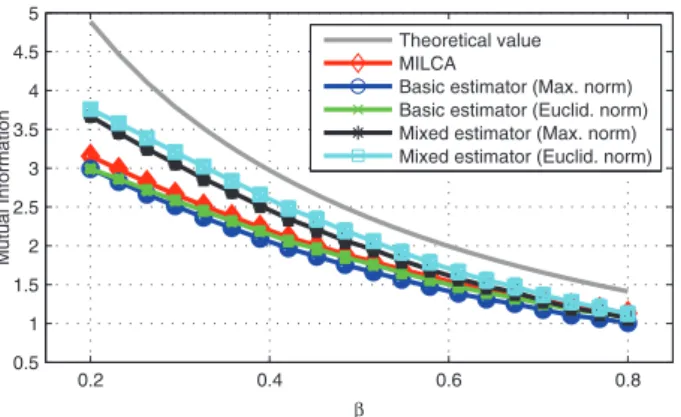
0.2 0.4 0.6 0.8 0.5 1 1.5 2 2.5 3 3.5 4 4.5 5 β Mu tu a l In fo rma ti o n Theoretical value MILCA
Basic estimator (Max. norm) Basic estimator (Euclid. norm) Mixed estimator (Max. norm) Mixed estimator (Euclid. norm)
(a) (Color Online) Mutual information (in nats) estimated with varying β, d = 3, n = 512. 256 362 512 724 1024 1448 2048 1.5 2 2.5 3 Signal length Mu tu a l In fo rma ti o n Theoretical value MILCA
Basic estimator (Max. norm) Basic estimator (Euclid. norm) Mixed estimator (Max. norm) Mixed estimator (Euclid. norm)
(b) (Color Online) Mutual information (in nats) estimated with different signals lengths, β = 0.4, d = 3.
0 1 2 3 4 5 6 7 8 9 10 ļ6 ļ5 ļ4 ļ3 ļ2 ļ1 0 1 Dimension Erro r MILCA
Basic estimator (Max. norm) Basic estimator (Euclid. norm) Mixed estimator (Max. norm) Mixed estimator (Euclid. norm)
(c) (Color Online) Mean estimation errorI(X, Y ) − I(X, Y ) (in÷ nats) with varying dimension, β = 0.5, n = 512.
FIG. 1. Mutual information and mean estimation error using the different estimators ÿI(X, Y )basic,E, ÿ
I(X, Y )basic,M, ÿI(X, Y )mixed,E and ÿI(X, Y )mixed,Mwith 100 trials.
denoted by ÿI(X, Y )mixed,E for the Euclidean norm and ÿI(X, Y )mixed,Mfor the maximum norm. Note that ÿI (X, Y )kbasic is obtained by replacing Eq. (32) by Eq. (23) in step (iii).
III. NUMERICAL TEST
The following linear model is generated
Y = X + β · e, (34)
where X and e are independent d-dimensional random vectors, and both of them follow a zero mean Gaussian distribution N (0, I) (I is the identity matrix). Clearly, when β decreases the dependence between X and Y in-creases. The theoretical value of the mutual information I(X, Y ) is equal to d
2log Ä1+β2
β2
ä
. For simulations we use
sequences of n independent samples (Xi, Yi) , i = 1, .., n from the distribution of (X, Y ).
We test the 4 estimators ÿI(X, Y )basic,E, ÿI(X, Y )basic,M, ÿ
I(X, Y )mixed,Eand ÿI(X, Y )mixed,M to estimate I(X, Y ). We also run the MI estimator algorithm freely available from the MILCA toolbox [8], simply denoted by MILCA, and which a priori corresponds to ÿI(X, Y )basic,M [9].
Throughout the experimentation, we choose k = 6 (the default k value of MILCA toolbox) for the basic estima-tors, and k1= 6, k2= 20 for the mixed estimators. The statistical mean and variance of the five estimators are estimated by an averaging on 100 trials.
Fig. 1(a) displays the performance of the five algo-rithms, for a given dimension (d = 3), a number of points equal to n = 512, and different values of β. The corre-lation between X and Y is all the more important as β is low. It comes out that all estimators are compara-ble when β reaches 0.8 (corresponding to a correlation coefficient around 0.78 between same ranks coordinates
6 of X and Y ). When the signals are highly correlated
(low values of β), the basic estimators still show identical behaviors, but, in this case, the two new mixed estima-tors clearly outperform the former whatever the norm, the best result being obtained using the Euclidean norm based estimator. Even if all results are not presented here, we find that the two new estimators outperform the basic ones using either k = 6 or k = 20.
We also tested the five estimators for different lengths of the time series for given values of β and d. As displayed in Fig. 1(b), the two new mixed estimators behave better whatever the length of the signals (ranging from 512 until 2048), the improvement being all the more important that the signal length is short.
When computing the error between the different es-timators and the theoretical value, for a given value of β (β = 0.5) corresponding to a correlation coefficient between the signals equal to 0.89, and an increasing di-mension, the same conclusion globally holds, as displayed in Fig. 1(c). The new mixed estimators clearly outper-form the basic ones (which display comparable behavior) especially for high dimensions. However, for very low dimensions (d = 1 or d = 2), the original estimators may be preferred. Clearly, for all estimators, the error grows along with the dimension, the best result being
systematically obtained with the mixed estimator based on the Euclidean norm. Since the standard deviations are quite low, they are not shown in these figures. Using the basic estimators (or MILCA), the standard deviation varies from 0.03 to 0.06 which is extremely low compared to the estimated values of mutual information (approx-imately from 1 to 5). As for the mixed estimators, the standard deviation varies from 0.04 to 0.09. The increas-ing in standard deviation can be considered as negligible in comparison to the accuracy of the estimation.
IV. SUMMARY
In this paper, we investigated the difficult issue of bias reduction on mutual information estimation. Once we established a relation between the systematic bias and the distance parameter for plug-in entropy estimator, two strategies, a basic one and a new one involving mixed estimators, were discussed. Experimental results allowed us to assess the performance of the new estimators using Euclidean or maximum norms to get a more accurate estimation of mutual information.
[1] T. M. Cover and J. A. Thomas, Elements of information theory (John Wiley & Sons, New York, 1991).
[2] A. Kraskov, H. St¨ogbauer, and P. Grassberger, Phys. Rev. E 69, 066138 (2004).
[3] S. Frenzel and B. Pompe, Phys. Rev. Lett. 99, 204101(2007).
[4] Q. Wang, S. R. Kulkarni, and S. Verd´u, IEEE Trans. Inf. Theory 55, 2392 (2009).
[5] K. Fukunaga and L. Hostetler, IEEE Trans. Inf. Theory
19, 320 (1973).
[6] K. Sricharan, D. Wei, and A. O. Hero III, IEEE Trans. Inf. Theory 59, 4374 (2013).
[7] K. Fukunaga, Introduction to statistical pattern recogni-tion, 2nd edition (Academic Press, San Diego, 1990). [8] http://www.ucl.ac.uk/ion/departments/sobell/Research/
RLemon/MILCA/MILCA
[9] The algorithm encoded in the toolbox [Eq. (2) or (3)] is not documented.