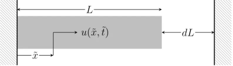
D'Alembert function for exact non-smooth modal analysis of the bar in unilateral contact
Texte intégral
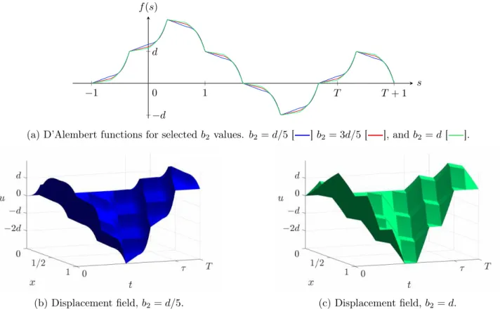
Figure
![Figure 2: Example of a 1CPP motion: u(1, t) [ ] and u x (1, t) [ ].](https://thumb-eu.123doks.com/thumbv2/123doknet/13013624.380802/4.892.253.639.406.595/figure-example-cpp-motion-u-t-u-x.webp)
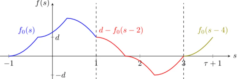
![Figure 3: A 1CPP motion [22] and corresponding d’Alembert function](https://thumb-eu.123doks.com/thumbv2/123doknet/13013624.380802/5.892.95.786.504.975/figure-cpp-motion-corresponding-d-alembert-function.webp)


Documents relatifs
We present a global error estimator that takes into account of the error introduced by finite element analysis as well as the error introduced by the iterative resolution of the
The penalty method is a classical and widespread method for the numerical treatment of con- strained problems, in particular the unilateral contact problems arising in mechanics of
As well as the Nitsche’s method for second order elliptic problems with Dirichlet boundary condition or domain decomposition [4], our Nitsche-based formulation (8) for
In this large deformation framework the exact solution is unknown: the error of the computed displacement and Lagrange multipliers are studied taking a refined numerical solution
Results of non-linear modal analysis; change in the natural frequency (a) and in modal damping (b) depending on the level of vibration.... asymptotic state for an
Although the NNM frequency of the systems with no initial gap between the solid body and unilateral constraint is energy in- dependent [14], we utilise the developed dynamic
It has been demonstrated that the net exchanged power transmitted from one oscillator to the other only depends on total energies of oscillators and of a ”modal coupling loss factor
Abstract: The contact between two membranes can be described by a system of varia- tional inequalities, where the unknowns are the displacements of the membranes and the action of
