Cooperative autonomous tracking and prosecution of targets using range-only sensors

Cooperative Autonomous Tracking and

Prosecution of Targets Using Range-Only Sensors

by

Arthur D. Anderson

B.S., Engineering Science and Mechanics, The Pennsylvania State

University, 2006

Submitted to the Department of Mechanical Engineering

in partial fulfillment of the requirements for the degrees of-._...

MASSACHUSETTS INSTITU)TE

Naval Engineer

and

_{MAY 3 0 2013}

Master of Science in Mechanical Engineering

at the

_L1BRARIES

MASSACHUSETTS INSTITUTE OF TECHNOLOGY

June 2013

©

Arthur D. Anderson, MMXIII. All rights reserved.

The author hereby grants to MIT permission to reproduce and to

distribute publicly paper and electronic copies of this thesis document

in whole or in part in any medium now known or hereafter created.

Author ...

...

Department of Mechanical Engineering

A^ _f

June 2013

C ertified by ...

.. . . . . .

.

John J. Leonard

Professor of Mechanical and Ocean Engineering

Thesis Supervisor

C ertified by ...

...

. ...

...

Michael R. Benjamin

Research Scientist, Deptment of Mechanical Engineering

plI0eis Supervisor

A ccepted by ...

...

David E. Hardt

Chairman, Department Committee on Graduate Students

Cooperative Autonomous Tracking and Prosecution of

Targets Using Range-Only Sensors

by

Arthur D. Anderson

Submitted to the Department of Mechanical Engineering on June 2013, in partial fulfillment of the

requirements for the degrees of Naval Engineer

and

Master of Science in Mechanical Engineering

Abstract

Autonomous platforms and systems are becoming ever more prevalent. They have become smaller, cheaper, have longer duration times, and now more than ever, more capable of processing large amounts of information. Despite these significant techno-logical advances, there is still a level of distrust for the public autonomous systems. In marine and underwater vehicles, autonomy is particularly important being that communications to and from those vehicles are limited, either due to the length of the mission, the distance from their human operators, the sheer number of vehicles being used, or the data transfer rate available from a remote operator to an underwater ve-hicle through acoustics. The premise for this research is to use the MOOS-IvP code architecture, developed at MIT, to promote and advance marine vehicle autonomy collective knowledge through a project called Hunter-Prey. In this scenario, two or more surface vehicles attempt to cooperatively track an evading underwater target using range-only sensors, and ultimately maneuver into position for a "kill" using a simulated depth charge. This scenario will be distributed to the public through academic institutions and interested parties, who will submit code for the vehicles to compete against one another. The goal for this project is to create and foster an open-source environment where parties can compete and cooperate toward a common goal, the advancement of marine vehicle autonomy. In this paper, the Hunter-Prey scenario is developed, a nominal solution is created, and the parameters for the scenario are analyzed using regression testing through simulation and statistical analysis.

Thesis Supervisor: John J. Leonard

Title: Professor of Mechanical and Ocean Engineering Thesis Supervisor: Michael R. Benjamin

Acknowledgments

I would like to thank the many people who have helped encourage me and support me in completing this thesis. Nothing worth doing is done alone, and this paper is certainly no exception.

Foremost, I'd like to thank Alon Yaari, who has been very patient in teaching me and working with me over the past year, and given me much advice and help through the various steps of this research. Thank you to Mario Bollini, who has been a major contributor to the regression testing code. I'd also like to thank Michael Benjamin, for his reading and editing and advice in the direction of this thesis, for his detailed notes and edits, and his enthusiastic support. And I'd like to thank my thesis adviser, John Leonard, who despite an extremely busy schedule, has found the time to advise and guide me throughout this whole process.

Last and most of all, I'd like to thank my colleagues, friends, and family, who have endured me being away for many hours at a time to work on my studies, and always supported me in more ways than I can mention here, so that I could always be my best. Without their support, none of this would have been possible.

Contents

1 Introduction and Background

1.1 The Need for Autonomy . . . . 1.2 The Hunter-Prey Project . . . . 1.3 Goals of Thesis Research . . . . 1.4 Current Literature Review and Comparison . . . 1.5 MOOS-IvP: The Code Architecture . . . . 2 Tracking with a Particle Filter

2.1 O verview . . . . 2.1.1 Step 1: Initialization . . . . 2.1.2 Step 2: Prediction . . . . 2.1.3 Step 3: Weight Calculation . . . . 2.1.4 Step 4: Resampling . . . . 2.2 Other Considerations . . . . 2.2.1 More Advanced Particle Filters . . . . 2.2.2 Reserve Particles . . . . 2.2.3 2D Tracking in the Hunter-Prey Problem . 2.3 PF Parameters . . . . 3 The Hunter-Prey Scenario

3.1 Mission Environment and Vehicles . . . . 3.2 Description and Rules . . . . 3.2.1 General Overview . . . . 13 . . . . 13 . . . . 15 . . . . 16 . . . . 16 . . . . 18 23 . . . . 23 . . . . 24 . . . . 26 . . . . 27 . . . . 28 . . . . 29 . . . . 29 . . . . 30 . . . . 3 1 . . . . 3 1 33 . . . . 33 . . . . 36 . . . . 36

3.2.2 Initial Set-Up . . . . 36

3.2.3 USV Range Sensor Rules . . . . 37

3.2.4 Depth Charge Rules . . . . 38

3.2.5 USV Communication . . . . 41 3.2.6 Mission Parameters . . . . 41 3.2.7 Scoring System . . . . 42 3.3 Nominal Solution . . . . 44 3.3.1 UUV Logic . . . . 44 3.3.2 USV Logic . . . . 45

3.3.3 USV Code Architecture . . . . 49

4 Regression Testing and Analysis 51 4.1 Goals of Testing . . . . 51

4.2 Variables and Description . . . . 51

4.2.1 Assumptions . . . . 53

4.3 Determining the Main Effects . . . . 54

4.4 ANOVA Testing Background . . . . 55

4.5 Testing Results . . . . 57

4.6 Results Analysis . . . . 63

4.7 Recommendations for Solution Improvements . . . . 66

4.8 The Future of Hunter-Prey . . . . 67

5 Conclusions 71

A Regression Testing Data 75

B Regression Results 79

List of Figures

1-1 Unmanned Systems' Key Components 1-2 1-3 1-4 1-5 1-6 2-1 2-2 2-3 2-4

Systems' Technology Maturity . . .

Bearing Only Tracking . . . .

Cooperative Positioning . . . . MOOS Database Tree . . . .

IvP Helm Structure . . . .

Particle Filter Overview . . . . Particle Initialization . . . . Geometry for Determining Weights Resampling Process Example . . .

3-1 Hunter-Prey Op-Box . . . . 3-2 Kingfisher USV and Bluefin-9 UUV Pictures 3-3 Sensor Probability of Detection by Range . . 3-4 UUV Random Waypoints Sample . . . . 3-5 Five Main Behaviors of the USV's . . . .

3-6 USV Searching Behavior Loiter Circles . . .

3-7 USV Code Architecture Diagram . . . . 4-1 ANOVA Tables for Main Effects . . . . 4-2 Effects vs. Standard Normal . . . . 4-3 Possible USV Sensor Arcs . . . .

. . . . 14 14 17 18 19 20 24 25 28 30 34 35 39 45 46 47 49 59 62 69 . . . . . . . .

List of Tables

2.1 Particle Filter Parameters Used in Testing Parameter Designators and Baseline . . . . . Sample DOE with Two Parameters . . . . . Regression Testing Parameter Values . . . .

Effects' Names and Values . . . . Interaction Effects . . . . Effects and P-Values . . . . The Statistically Significant Effects... Average Misses for Depth Charge Parameter

. . . . 52 . . . . 53 . . . . 58 . . . . 58 . . . . 59 . . . . 61 . . . . 63 V alues . . . . 65

A.1 Parameter Values by Simulation . . . . B.1 Results from Regressions 1 and 2 . . . . B.2 Results from Regressions 3 and 4 . . . . C.1 ANOVA Tables for Interaction Effects . . . . 75 . . . 79 . . . 83 87 4.1 4.2 4.3 4.4 4.5 4.6 4.7 4.8 32

Chapter 1

Introduction and Background

1.1

The Need for Autonomy

The focus of this research is Marine Vehicle Autonomy, Communication, and Cooper-ation. Autonomous platforms and systems, in both the military and the commercial worlds, are becoming ever more prevalent. They have become smaller, cheaper, have longer duration times, and now more than ever more capable of large amounts of information. Ships are being designed with less and less manning, and unmanned vehicles, either in the air or in the water, are being used for numerous applications today. All these are trends toward systems with greater amounts of autonomy with less human input [2].

This progress is due to a number of different reasons. Advances in battery tech-nologies have allowed autonomous platforms to stay out for longer periods of time. Sensors, such as GPS and sonar, are becoming smaller, cheaper and more capable. And computing power, which used to be a highly limiting factor in marine autonomous systems, can get the same and better performance for significantly smaller size and less electrical power. Acoustic communications have also made significant advances in recent years. Figure 1-1 depicts these key components necessary for fielding au-tonomous marine vehicles, while Figure 1-2 shows how these different technologies, which are still very much in the process of developing and improving, have matured over the past 18 years. These advances in the critical components are what drive the

Figure 1-1: There are several key technology components that must mature for effec-tive unmanned marine systems to be developed

[1].

Critical - C''""'- a!L! -

---kII iIf tII

Con"t _-In

I 1-11Hl

camcheneWeMe semrtfcaovry s.srs chanerys s.OrWA

LsMwu Swon Smchbfw I W

compute-Power ompwAr c wer

Tm-:--- .-- ...

1995 2005 2012

Figure 1-2: Over the past 18 years, the technology capability of the key components for unmanned marine systems has improved significantly. The advances in the other key components drive what is expected from autonomy [2].

expectations of marine autonomy [2].

Despite these significant technological advances, there is still a level of distrust

for human operators in autonomous systems, as they are often seen as unreliable or

incapable of making important decisions without human input. Autonomy, however,

is particularly important especially in the case of marine and underwater vehicles.

Communication from those vehicles is often limited, either due to the length of the

mission, their distance from human operators, the sheer number of vehicles being used, or the data transfer rate available from a remote operator to an underwater

vehicle through acoustics [2].

This gap of trust must be crossed if we are to continue the path of fielding more

in-crease the self-reliance of these autonomous systems, and to facilitate a greater trust and understanding for both military and industry in using autonomous vehicles to accomplish their tasks.

1.2

The Hunter-Prey Project

The premise for the Hunter-Prey project is as follows: using the MOOS-IvP code architecture developed at MIT for autonomous marine vehicles, a set of rules will be created for a hunter-prey type scenario, in a way that two or more surface vehicles attempt to track an underwater target using range only sensors. The vehicles will attempt to maneuver in such a way that maximizes their sensing capability of the underwater vehicle and also maneuvers the vehicles into a position for a "kill", using a simulated depth charge, explained later in Chapter 3. The vehicles in play will have limited communication between themselves and a remote human operator.

This scenario and set of rules will then be distributed to a number of different academic institutions and interested parties, who will submit ideas and algorithms to dictate the vehicles behavior, whose performance will be numerically graded and analyzed (also explained further in Chapter 3). These algorithms will be judged based on their ability to track and find an underwater target, as well as the ease of their operator interface with the autonomous system.

The overall project will attempt to accomplish three main goals. First, it will create and foster an open-source environment where many parties can compete and cooperate toward a common goal, which may be useful when more realistic scenarios could be developed and require solutions. Second, it will allow us an in-depth look as to what sort human input is optimal in an environment where human input and communication is limited, and third, how solutions should be shaped in the future. Finally, it will help contribute to the open-source MOOS-IvP code already developed in depth for future potential research and applications.

1.3

_{Goals of Thesis Research}

This goal of the research in this paper is to create baseline upon which the Hunter-Prey project can build. More specifically, this thesis will seek to: 1) define the rules, guidelines, and set-up for the Hunter-Prey scenario, 2) develop a "straw-man" or basic solution to the problem, and 3) run this solution through regression testing to determine which factors, such as sensor capabilities or vehicle speed, affect the problem, and by how much. Lastly, 4) this project will discuss the ways to move forward with the project as it moves toward becoming an open competition. This will allow for a greater understanding of how the parameters affect the problem so we can better set them for the competitors for the more general Hunter-Prey project. The method presented for scoring in this research will also provide a framework for understanding how to measure the success rates of more complex problems, such as including actual acoustic signatures, multiple path returns, and tracking multiple targets, as they are developed.

The solution to the Hunter-Prey problem presented in Chapter 3 is not an opti-mized solution, but is intended to be a baseline solution that can be used by partici-pants in the Hunter-Prey project for their submissions. Where specific improvements can be made to the algorithms for the vehicles are discussed in Section 4.7, but the searching for a more optimal solution is not the goal of this research.

1.4

_{Current Literature Review and Comparison}

The major difference between this paper and papers that attempt tracking problems is the measure by which success is determined. Other research papers, when evaluating the effectiveness of a range-only tracker or solution, use a least squares measurement of the detected target track against the actual target track. For example, in 2006, a paper by Donald P. Eickstadt and Michael R. Benjamin explore using bearing only sensors to track a target vehicle [7]. In this study, two tracking vehicles do loitering circles, while a third vehicle, the one being tracked, passes between them,

Figure 1-3: Two tracking vehicles conduct loiter circles while a target vehicle tracks between them. The tracking vehicles are using bearing only sensors to attempt to localize the target [7].

as the tracking vehicles attempt to use their sensors to localize the third vehicle as illustrated in Figure 1-3. As we can see from the figures, the accuracy of the tracking algorithm is measured through a least squares estimation.

This is illustrated in another study. In 2010, Gao Rui and Mandar Chitre wrote a paper in which one autonomous vehicle with the ability to locate itself with a high degree of accuracy using GPS, and another vehicle could only find it's position through less accurate dead reckoning [14]. Using range-only measurements between the two vehicles, the vehicle with dead-reckoning tracking is able to obtain a significantly higher degree of accuracy in it's own position, as shown in Figure 1-4. Again, the method for determining success was using a least squares measurement to determine error.

In this paper and the overall Hunter-Prey project, however, the defining principle is not a measurement of positional error, but the measure of overall mission success. This is done because the Hunter-Prey concept is more complex than these developed scenarios and therefore positional error would be more difficult to analyze, and also, more importantly, because the goal of this research is to look at how the range-only tracking problem posed affects the success of the mission, which ultimately is the goal for fielding autonomous vehicles.

It should also be noted that previous work has been done on improving particle filter and other tracking algorithms. For example, in 2013, Guoquan P. Huang and

_JA I=J -A 0 100 M1 1

Ease (0n) WM ()

Figure 1-4: Two vehicles, one with good navigational data and the other not, commu-nicate using only range data between them to help localize the vehicle with inferior navigation [14].

Stergios I. Roumeliotis wrote a paper which looks at using a Gaussian mixture based approximation proposal distribution, allowing for slower depletion of particles [9]. The range-only tracking in this solution is solved using a particle filter code devel-oped for MOOS-IvP [13]. This a basic particle filter, and this research doesn't seek to find methods to improve it's performance. In this way, the research can focus on the creation of the project and analysis, instead of researching better particle filter algo-rithms. Better particle filters can be worked out by competitors making submissions for the Hunter-Prey Project, but is outside the scope of this thesis.

1.5

MOOS-IvP: The Code Architecture

The code architecture to be used for the Hunter-Prey project is based on an open source project called MOOS-IvP. Launched originally at MIT in 2005, MOOS-IvP includes more than 150,000 lines of code and 30+ core applications dedicated to controlling marine vehicles, mission planning, debugging, and post-mission analysis. This software has been run on over a dozen different platforms and is being used at the Office of Naval Research (ONR), the Defense Advanced Research Projects Agency (DARPA), and the National Science Foundation programs at MIT. MOOS-IvP can be used for a simulated environment, or for fielding the vehicles in a real environment.

I

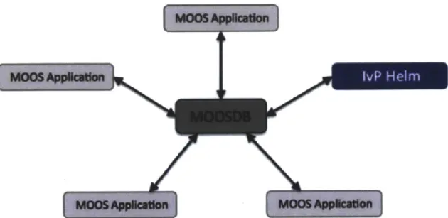
Figure 1-5: A MOOS community is a collection of MOOS applications, each publish-ing and subscribpublish-ing to variables published to the MOOSDB. A MOOS community typically operates on a single vehicle or computer. [2].

The MOOS portion of MOOS-IvP stands for "Mission Oriented Operating Suite", and contains a core set of modules that provide a middleware capability based on a publish-subscribe architecture. Processes in the MOOS database are defined by what messages they subscribe to (publications), and what messages they consume (subscriptions). The key idea for MOOS is that it allows for applications that are mostly independent, and that any application can be easily replaced or upgraded with an improved version with the requirement that only its interface match [2]. Figure 1-5 shows a MOOS community, which typically runs on a single machine, and the structure of processes. MOOS communities set-up on different vehicles are also

capable of communicating with one another.

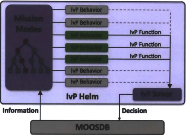
The IvP portion stands for Interval Programming, and is a single MOOS appli-cation that runs inside the MOOS database. IvP uses a behavior-based architecture for implementing autonomy. These behaviors are distinct modules that are each ded-icated to a specific aspect of autonomy, for example, following a set of waypoints or collision avoidance. If multiple behaviors are active, the IvP uses a solver to rec-oncile the desires of each behavior using an objective function, or IvP function [2]. Figure 1-6 shows how the IvP system structure is structured.

InformIiofl

I -s___

Figure 1-6: The IvP helm is a single MOOS application. It uses a behavior-based architecture in which uses a mode structure to determine which behaviors are active. Each of the active behaviors are then reconciled using a multi-objective optimization solver, or the IvP solver. The resulting decision is then published to the MOOS database [2].

Many existing behaviors already exist as part of the open MOOS-IvP software available. These behaviors a fully leveraged in this project: all behaviors used in this research have already been created and documented in the available MOOS-IvP documentation [2]. The specific behaviors used are discussed in Chapter 3.

Chapter 2

Tracking with a Particle Filter

2.1

Overview

Tracking with a sensor that gives you only ranges can be a difficult problem, although it is certainly not a novel one, and many methods have been used to explore this problem.

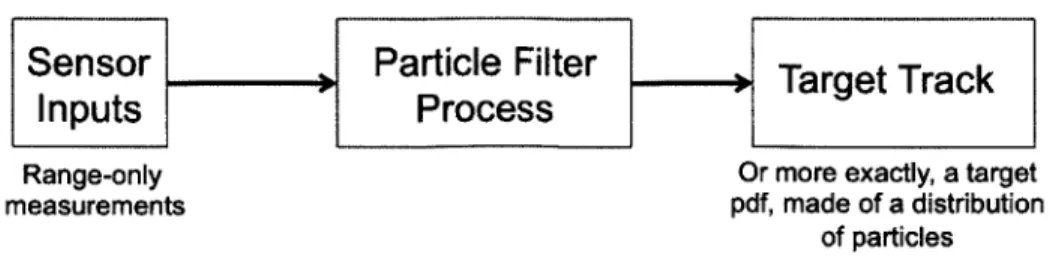
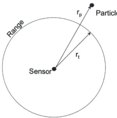
This problem is solved using a particle filter, also known as a Sequential Monte Carlo (SMC) method, which is a means of developing target solution using observa-tions from sensors. In the case of the Hunter-Prey problem, this data is in the form of range-only information. A PF simulates possible solutions, or particles, that fit the range observations made, and then readjusts and updates as more information is obtained. If enough particles are generated, the distribution of particles can represent a continuous probability distribution function (pdf) of the target's position. A simple way to think of a PF can be thought of as a method for developing a track solution based on range information, as illustrated in Figure 2-1.

A PF has 4 steps. The first step, called initialization, generates all the particles, and occurs when the first range measurement is received. Each particle can be thought of as a guess as to the position and velocity of the target track. When the next range observation of the target is received, each of the particles, of track guesses, are evaluated based on the new information, and new, more accurate particles can be evaluated if needed. More specifically, upon receiving a new range measurement

Sensor

_{, Particle Filter _-+Tre}

_rc

Inputs

ol

Process

0TreTac

Range-only Or more exactly, a target measurements pdf, made of a distribution

of particles

Figure 2-1: The particle filter takes a set of measurements or inputs, and produces a target track.

after the first one, the PF advances the particles to where they would be based on their previous states (step 2), assigns each of the particles weights (step 3), and then checks to see if enough particles have degraded to the point where they need to be resampled (step 4). After each new range measurement is received, steps 2, 3, and

4 are repeated. The following sections describe in greater detail each of these steps

and how they are completed.

2.1.1

Step 1: Initialization

When the first range measurement is received, N particles are generated, all at the received range. Each particle is given a Cartesian coordinate:

Xi = [xi, i, ]T (2.1)

such that

i= rt sin(#5) cos(64) for a random:

y= rt sin(#j) sin(64) -7r/2 <= #i <= 0

zi= rt cos(#i) 0 <= 64 <= 27r

This creates i = 1, 2, ..., N particles such that they are randomly distributed in

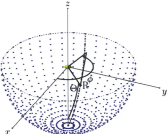
a hemisphere below the source (because the target will either be at or below the depth of the vehicle) at the range rt received by the range sensor at time t. Here,

#

Figure 2-2: A set of N particles randomly distributed at a range rt from the sensor. This is what the particles distribution will look like after initialization [13].

i = [±i, i, ziT (2.2) such that: 2k = vi sin(<i) cos(E9)

9j

- r/2 - <bmax <= <bi <= 7/2 + <bmax In the above equations, <b represents the elevation angle of the target,

E

I

This equation shows the state of the particle. Stepping back, we see that a number of particles have been generated randomly in a hemisphere below the point source, as shown in Figure 2-2.

2.1.2

Step 2: Prediction

Once the particles have been initialized and then a second range measurement or observation has been received, the particles must be advanced to the new positions. The equations by which the particles advance is simply to use each of the particles po-sitions and velocities from the state Equation 2.3, and the time At difference between this report and the last report.

t t-1 *t

yi =yi ±y, At

Y t-1 +*t- lAt

After we advance the particles, in preparation for the next step, noise must be inserted into each of the particles' velocities. This is done for two reasons. First, as we will see in Section 2.1.4, because we will draw new particles from old ones as some particles become degenerate, we want to create some variation such that all the particles are not the same particle. Secondly, if the target track changes heading, elevation angle, or velocity magnitude, we want the particles to be able to follow the target, and this can only be done of some particles are allowed to deviate from their previous velocity state.

How much noise needs to be added is a careful consideration when using a PF. Adding too much noise will cause the particles to go off in many directions, and make it less able to follow a target going in a straight line and constant speed. On the other hand, if not enough noise is added, it may take several time steps before a single particle is able follow a target track going through a sudden speed or velocity change. For the purposes of this paper, the values heuristically determined in Andrew Privette's paper were used [13]. These values are listed in Table 2.1. One solution to the problem of not enough noise to follow a track is the use of reserve particles, discussed in Section 2.2.2

The following is the process for adding noise. First, separate the velocity vector *i into velocity, heading and speed:

tan-( o'-1 - tan-'

Next, add noise to each of the parameters:

S= -+Vnoise+

e0=

+enoise

(D 4It- + 4Dnoise

Finally, translate these back into the original velocity vector to describe a new state:

zi

yi

ii = vi cos(Gi )

This new velocity vector is used to describe the particles at the next time step t, This, along with the new position vector from Equation 2.1, fully describes the new state of the particles.

2.1.3

Step 3: Weight Calculation

When the particles have been advanced, we then compare their positions to the range

rt measured from the sensor. We do this by by using an importance factor, or weights,

where the weight of a particle represents how likely the particle might be the actual target track given the range observations made. The equation used to determine the weights is:

S=i_1p(rt|Cl)p(C(|C-1) (2.4)

* i _{q ((it|I(j , rt)}

here, p((l- 1) _{is known as the transition prior and q(Qtj(?:t, rt) is called the} importance function, and for convenience we set them equal [11]. This allows us to simplify the weight equation to:

Particle

Figure 2-3: The variables measured geometrically for the determination of weights.

w= w- 1p(r

l)

From this equation, we find that the weight of each of the particles is based on the weight from the prior time step, and the probability of the state of the particle

rt given (. _{We approximate this distribution as a normal distribution.}

2.1.4

Step 4: Resampling

As new range information comes in, it will become apparent that many of the particles will be less and less likely. Many particles will be found to just completely incorrect by being completely off from the new range, while some may fall directly on it. If enough accurate information comes in, it may be likely that only one or two of the particles are the most likely solution. This is called particle degeneration, and in order to prevent this, we resample.

The first stage in resampling is to determine whether or not resampling is neces-sary. To do this, the effective number of particles is calculated using Equation 2.6. If the effective number of particles Neff is lower than a set threshold Nthreshold, then

a resampling is performed. Nthreshold is generally set to half the number of particles N/2.

Neff N '(26)

E_1 (w )

where

N Nthreshold 2

Resampling is then performed based on the weights of the particles. N new par-ticles are drawn from the old set, but parpar-ticles with higher weights are more likely to be drawn from than particles with low weights. In other words, if a particle has a high weight, then many of the particles of the new set will have the same velocity as the old, higher weighted particle from the previous set.

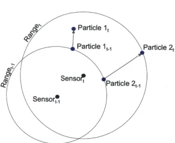
This idea is illustrated well in Figure 2-4, for two particles. At time t - 1 each of the particles will have a very high weight because each particle falls on almost the exact range measured by the sensor. However, when new range information is received at time t, Particle 1 is found to be off the range, will be calculated to have a lower weight, and will much less likely to be resampled if resampling will occur at this step. Particle 2 however, will have a high weight at time steps t - 1 and t, and therefore will be much more likely to be drawn from in the next resampling process. After N new particles have been drawn, the old set is dropped, and each of the new particles is given an equal weight of 1/N. These are the particles that will be evaluated at the next time step, when the next new range measurement is received, and the steps are repeated.

2.2

Other Considerations

2.2.1

More Advanced Particle Filters

It should also be known that more extensive particle filtering methods have been developed than he basic particle filter developed for this problem. For example Huang and Roumeliotis in their paper build the probability density function of particles

Figure 2-4: Two particle moving being evaluated at initial time t - 1, and then again at time t.

based on an analytically determined Gaussian pdf rather than an assumed one, which helps reduces the rate of particle depletion [9]. The particle filter could also be improved by analyzing the values used for variance, noise, particle count, reserve particle count, and other parameters. The numbers used in this algorithm were determined empirically, however, using more optimal numbers, or even writing an algorithm that would allow the vehicle itself to calibrate these values autonomously could be highly beneficial [13].

These solutions, while they would certainly lead to better and more efficient track-ing, are not used for the purpose of this research, as the goal is only to create a simple "straw-man" solution and then analyze it as discussed in section 1.3. Better filters and algorithms should be the subject of further research, and for submissions to the Hunter-Prey competition.

2.2.2

Reserve Particles

One additional tool used in PF Tracking is the use of reserve particles. When all the particles are resampled, the new particles have the velocity vectors of the old particles from which they are drawn, with some random noise added so that new particles which are drawn from the same old particle are not exactly the same. But

if the contact decides to make a sharp turn, this could be a problem for particles attempting to track that turn. For example, is the maximum turning noise was 15 degrees, and the target being tracked turned 60 degrees, it would take the particles at the end of that turning spectrum at least 4 time steps to get to the correct bearing, and by that time, the particles will have made a wider turn than the vehicle, and now need to speed up to catch it.

In order to resolve this problem, reserve particles are used. During the resampling process, these particles are drawn from the the old set similarly to how the previous set was drawn, however, now these vehicles are given a random velocity vector. This way, when the target makes a sharp turn, some of the reserve particles are likely to closely reflect that turn, and are able to track it. These particles should be a minority compared to the other particles, and how many to use exactly is something to be considered. Too many reserve particles means more noise will be generated in tracking a vehicle moving in a straight line, but not enough reserve particles will make it more difficult to catch sharp turns.

2.2.3

2D Tracking in the Hunter-Prey Problem

There are several other factors that come into play when dealing with the specific Hunter-Prey problem. The first is that the problem, as described in greater detail in Chapter 3, is generally presented and solved in 2 dimensions only. This signifi-cantly simplifies the particle filter task, in that only X and Y position and velocity components need to be generated. This also means that fewer particles need to be generated in order to achieve an accurate solution.

2.3

PF Parameters

A number of parameters have been mentioned over the course of this chapter, such as the number of particles and the random noise, all which may be tweaked and adjusted in tests. for maximum effectiveness. While a rigorous test was not performed on the PF for the Hunter-Prey project, a series of informal trial and error tests were

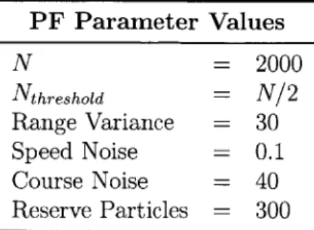
performed to obtain a good, working solution. Table 2.1 shows the parameters used for tracking in this particular problem:

PF Parameter Values N = 2000 Nthreshold = N/2 Range Variance = 30 Speed Noise = 0.1 Course Noise = 40 Reserve Particles 300

Table 2.1: A list of the parameters used and their values for the particle filter for this research in the Hunter-Prey scenario.

Chapter 3

The Hunter-Prey Scenario

With the understanding of the particle filter and how a vehicle is able to track with range-only information, the next step is to address the full Hunter-Prey scenario scenario. This chapter will discuss how the scenario rules are established, and also provide a set of logics or algorithms that demonstrates a basic solution of how this scenario could be solved from both sides of the problem. This is the solution that will be tested and analyzed in Chapter 4, with an exploration into how each of the parameters set for the problem affect the outcome of the scenario.

3.1

Mission Environment and Vehicles

The Hunter-Prey Scenario has been designed so that it will work inside an operating box (or op-box) within the wi-fi coverage area of the MIT sailing pavilion on the Charles River in Boston. Figure 3-1 shows a satellite picture of how the op-box is situated within the wi-fi area. This is the facility from where MIT's vehicles are launched, and has sufficient area to conduct the full mission. The op-box area within the wi-fi area was chosen to be large enough to conduct the mission, but no so large as to interfere with traffic on the South side of the river.

While the underwater vehicle in the scenario will be submerged, the Hunter-Prey problem is being treated as two dimensional. All participating vehicles and ranges are given locations only in the X-Y plane. This not an unreasonable assumption

Figure 3-1: The op-box for the Hunter-Prey scenario on the Charles River by the MIT Sailing Pavilion. The orange area represents the wi-fi coverage area, while the blue box represents the op-box. The white dots represent virtual poles, which mark starting positions and waypoints for the vehicles.

Figure 3-2: Left: A Kingfisher M200 Unmanned Surface Vehicle (USV) and Right: a Bluefin-9 Unmanned Underwater Vehicle (UUV).

because the Charles River is not particularly deep, the maximum depth being only 12m [10]. And during operation, the UUV will only operate a few feet below the surface. Under this set of rules, a surface vehicle may occupy the same X-Y position as an underwater vehicle, but two surface vehicles may not.

The surface vehicles being used for this mission are Kingfisher M200 USV's. These vehicles are made by Clearpath Robotics, and are the primary research surface ve-hicles used at MIT. They are relatively inexpensive, are driven by a ducted water jet propulsion system to a maximum speed of 2.0 m/s, and at 64 lbs, are easily launch-able by a single person. Most importantly, they are "autonomy-ready" and can be governed by software developed within the MOOS-IvP architecture. All these features make them an ideal candidate for testing in the Hunter-Prey scenario [6].

The UUV for this mission is a Bluefin-9, which is a lightweight, two-man-portable autonomous underwater vehicle equipped with a side scan sonar and camera. It has multiple navigational sensors, including GPS, a DVL, a CT sensor and a compass, that allows for less than 0.3% error for the distance traveled underwater. Like the M200 USV's, the Bluefin-9's maximum speed is 2.0 m/s, and most importantly the bluefin-9 is capable of accepting a number of different autonomy architectures, including MOOS-IvP [5].

3.2

Description and Rules

3.2.1

General Overview

In this scenario there are three vehicles, two USV's, which are named Archie and

Betty, and the UUV, which is named Jackal. The objective of the scenario for Jackal

is to start at one of the 5 virtual poles at the west end of the box, travel to one of the poles at the east side of the op-box, and then return to the finish, again, at one of the poles on the west side. The poles are waypoints on the edge of the op-box area, and are illustrated in Figure 3-1. It must do this while trying to avoid the USV's which are attempting to detect and "kill" Jackal using a simulated depth charge.

The goal for Archie and Betty is to prevent Jackal from completing its traversal. To do this, they have two tool at their disposal: each have a range-only sensor and a number of simulated depth charges. In order to stop Jackal, the USV's must drop a depth charge on top of Jackal. The depth charges, once dropped, have a set time delay before they "explode". If at the time of the explosion Jackal is within the range of the depth charge, then Archie and Betty have completed their goal, and the mission ends. The following sections discuss the rules and guidelines for how this scenario is set up.

3.2.2 Initial Set-Up

After all the vehicles are launched form the MIT sailing pavilion, and connect with the MOOS database, a deploy signal is sent from the shoreside computer, which orders the vehicles to travel to their starting positions. Note that there are 5 'poles' labeled on either side of the op-box in Figure 3-1. Upon receiving this command, Jackal submerges and traverses to any of the 5 poles on the west-side, whichever the vehicle so chooses, while Archie and Betty traverse to the east side. Archie's starting position is at the North-East corner of the op-box, or the top East pole, while Betty's is at the South-East corner, or the bottom East pole. All the vehicles then wait at their starting positions until the end of a designated time-period, at the end of which

will signal mission start. Figure 3-1 shows the corners of the op-box, as well as the positions for each of the poles.

At the mission start the USV's may begin to search for Jackal, while Jackal may begin its traverse. Jackal must start at one of the 5 poles on the west side of the op-box, pass through one of the poles on the east side, and then finish at any of the poles back on the west side again. During the entire scenario, Jackal is confined to operate only inside the op-box. Archie and Betty have somewhat more free range, and may travel outside the op-box, although they must stay well within the confines of the wi-fi coverage area. They must also at all times never close within 10 meters of each other for safety purposes.

3.2.3

USV Range Sensor Rules

In order to locate the Jackal, Archie and Betty each have a range sensor, which give the range between the vehicle with the sensor and the target. For simulation, the range sensor is simulated on the shoreside by a MOOS application called

uFidCon-tactRangeSensor

[4).

this message request is as follows:

CRSRANGEREQUEST = name=archie,target=jackal

This request will be received by the uFldContactRangeSensor application, which will determine if enough time has passed since the last request, as specified by the mission configuration parameters, and if the target is within range of the requesting vehicle's sensor. If both these conditions are met, the uFldContactRangeSensor ap-plication will pass back the jackal's range from the shoreside (simulated sensor) to the requesting vehicle in the following format:

CRSRANGEREPORTARCHIE vname=archie,range=30,

target=jackal, time=68162

Because the Hunter-Prey problem is two dimensional, ranges from the requesting vehicle to the target are given in the x and y planes only (depth is not considered in

the range).

For the purposes of this project, a modified uFldContactRangeSensor application has been created that allows for some chance in the sensing, as well as the ability to limit the sensor to certain sectors around the the vehicle.

As configured normally, the uFldContactRangeSensor looks at the range between the sensor and the target, and determines if this is less than the pull distance plus the push distance, and if it is, returns the range. However, in order to create another element of probability into this scenario, and also to more closely simulate an acoustic environment, a modified version of the application was used. In this scenario, the range sensor looks at the pull distance plus the push distance, adds the two together to create a maximum sensor distance, and then uses the following equation to determine the probability of detection:

3(Max - d)

Probability = e \ Max

)

Where Max is the pull distance plus the push distance, and d is the distance from the sensor to the target. Beyond the Max distance, the probability of detection decays exponentially. This equation can be shown graphically in Figure 3-3 for a

Max of 50 meters.

3.2.4

Depth Charge Rules

Depth charges are simulated by the uFldDepthChargeManager application run on the shoreside. Each vehicle is given a certain number of depth charges as specified by the mission parameters. In order for a specific vehicle to drop a depth charge, that vehicle must send a message in the following format:

DEPTHCHARGELAUNCH = vname=betty,delay=20

where vname is the name of the requesting vehicle, and and delay is the requested delay for the depth charge. Upon receiving this message, the

Range Sensor Detotion Probablity 0.9-Push + 0.8 - Pull Distance 0.7 -

0.6-Detection Probability Curve 0.5- 0.4- 0.3- 0.2-0.1 -01 0 20 40 60 80 100 120 140 160 180 200

Sensor to Target Distance

Figure 3-3: This graph shows the probability of receiving a range report on the

target given the distance between the sensor and the target. Below the push plus pull

distance, or Max, The probability is 100%. At greater ranges, the probability decays

charge, if the delay requested for the depth charge is at least the minimum required by the mission parameters, and finally if the vehicles still has any depth charges. If both these conditions are met, a simulated depth charge is be generated, with the delay specified by the user, and a blast radius as specified by the mission parameters. This Hunter-Prey problem is two dimensional, so the the simulated explosion radius is a circle on the horizontal plane surrounding the drop location.

If a surface vehicle wishes to see how many depth charges it has left, and the status of the depth charges it has already launched, it may send the following request to the uFldDepthChargeManager application:

DEPTHCHARGESTATUSREQ = vname=archie

The uFldDepthChargeManager will receive this request and send a reply in the following format:

DEPTHCHARGESTATUSARCHIE = name=archie,amt=3,range=25,

launches-ever=2,

launches-now= 1,hits=2

If the vehicle has used up all it's depth charges and wishes to get more, it must return to the MIT Sailing Pavilion, marked by the point X = 0, and Y = 0, and then send a request to uFldDepthChargeMgr in the following format:

DEPTHCHARGEREFILLREQ = vname=betty

If the vehicle is within 20 meters of the refill range, a counter will begin, and after a certain amount of time has passed (mission parameter Ref iliTime) with the vehicle remaining in range, the vehicles Depth Charge Supply will refill to the maximum amount the vehicle started with. During the refill period, a message will be passed in one of the following formats, depending on the status of the refill:

REFILLSTATUSARCHIE = vname=archie,status=refilling, time-remaining=45.37 REFILLSTATUSARCHIE = vname=archie,status=complete, time-completed=6532 REFILLSTATUSARCHIE _{= vname=archie,status=FAILED,} reason=moved-out-of-range

The first message of the three options above occurs if the vehicle has requested a refill, is in range, but has not yet been near the MIT Sailing Pavilion long enough to receive the depth charges. The second is posted when the vehicle successfully receives the refill, and the third occurs if the vehicle's refill failed because either the vehicle was out of range when the request was sent, or moved out of range between the requested time and the successful completion of the refill.

3.2.5

USV Communication

For this scenario, communication is unlimited, and mail may be passed back and forth between Archie and Betty using the uFldNodeComms application. Jackal does not communicate with the other vehicles.

3.2.6

Mission Parameters

The previous couple of sections mentioned "mission parameters" These are variables, such as the speed of the USV, used to describe how the mission is played out. The following is a list of the mission parameters that may change or be defined differently for a given runs.

1. Sensor Range: The maximum range at which sensor can sense Jackal 100% of the time.

2. Sensor Frequency: The time alloed between range sensor pings. 3. USV Speed: The maximum speed for Archie and Betty.

5. Depth Charge Range: The explosion radius (2D) of te simulated depth charges.

6. Depth Charge Amount: The starting number of depth charges for Archie and Betty, and maximum amount allowed to be held for the duration of the scenario.

7. Depth Charge Refill Time: The time vehicle must remain within 20 meters of the refill point in order to refill depth charges to the amount established by Depth Charge Amount.

8. Depth Charge Delay: The time following the depth charge drop, before the depth charge explodes.

9. Start Time: The time specified between when the vehicles are given the deploy command, and when the mission starts, giving the vehicles time to pre-position themselves at the start.

These mission parameters can be changed for different missions, and the first seven of these will be varied during the regression testing of the Hunter-Prey to determine what values of the parameters will be used for the Hunter-Prey Competition. Because many of these variables are simulated even during real water testing (such as depth charges), they are not limited by constraints. The exception, however, are the USV Speed and UUV Speed parameters, which are limited by the maximum speeds of the vehicles being used in the water. Both USV Speed and UUV Speed can be set no higher than 2 m/s.

3.2.7

Scoring System

In order to create a simple point around which we'll optimize the system, a grading system was created. Basically, the system starts at 200 points, and then users are penalized as time passes, and for each missed depth charge that is dropped. The following is the scoring equation:

where C1 is the miss multiplier, C2 is the time multiplier, and TMax refers to the time when the time penalty begins to be applied. These variables are configured by the scorer. The miss multiplier is the number of points lost in the scenario for a given depth charge miss, and the time multiplier is the number of points lost per second after the specified TMax constant. Misses refers to the number of depth charges dropped that detonate and do not hit the UUV, and only refers to misses prior to the hit. After the UUV is hit, the mission is over and all the vehicles are returned to the MIT Dock. TMax refers to the time between mission start and the first depth charge that detonates within the range of the UUV, measured in seconds. The score is capped at 200. The values used for these constants for this research are as follows:

C1 5

C2 = 0.1

TMax 150 (3.3)

Plugging these values into Equation 3.2, and we have the general scoring equation used for the Hunter-Prey scenario:

Score = 200 - 5(Misses) - 0.1((TimeToHit) - 150) (3.4)

For the purposes of this research, Equation 3.4 will give a single value which can be evaluated given the mission parameters. In the general Hunter-Prey project that will become an open competition, this will will help to provide weights based on the penalties of each. For example, with the constant values specified in the equation above, one depth charge miss is equivalent to 50 extra seconds of mission time in terms of mission score. This is important when writing autonomy code, because the vehicle will need to decide how much time it will want to take to make sure it has enough accuracy and good enough position to drop the depth charge, or if it wants to drop depth charges at will in the hopes that one will hit. How these constants are defined can greatly change the motivation of the autonomy decision making process.

3.3

Nominal Solution

In order to test the different Mission Parameters, a nominal solution was developed to the problem, which was subjected to regression testing. The following sections described the basic solution to the problem - the logics and algorithms that were applied to the vehicles to compete against one another based on te rules set forth in Section 3.2. This solution is not optimized, but was only developed to test the difficulty given a certain set of mission parameters.

3.3.1

UUV Logic

The UUV at this time has no knowledge of where the USVs search for it are. So, the solution was developed using the waypoint behavior, which allows a vehicle to traverse along a set of randomly generated waypoints. Jackal randomly determines which of the 5 poles on the left hand side to start from, and then steers towards that point after the deploy command is given. At the mission start, Jackal begins to traverse the op-box via the generated set of waypoints. The waypoints on the way to the east side are placed at the quarter, half, and three-quarter marks in the East-West

direction across the op-box, but are chosen randomly on the North-South. Then a pole is randomly selected for the east side of the op-box for the next waypoint, and then the vehicles uses a similar method for the return. A sample set of waypoints is shown in Figure 3-4.

For future iterations of the Hunter-Prey project, Jackal will have a method to detect the USV's, for example, by knowing the position of the surface vehicles when they ping. This could create more interesting, and more complex, scenarios where the UUV can attempt to maneuver away from the surface vehicles, and where one of the surface vehicles may desire to stop pinging, or "go quiet", in order to mask their position from Jackal. However, for the purposes of keeping this solution and project within a reasonable time-frame, the current waypoint logic will be used without an avoidance behavior.

1/4 1/2 3/4

West Side East Side

Start

End

--- --- L---5.---5. --- 4

Figure 3-4: An example randomly generated path for Jackal.

3.3.2

USV Logic

Archie and Betty have a somewhat more complex set or rules than Jackal. While in operation, the two vehicles have five basic modes in which they operate: Start, Re-supply, Search, Track, and Prosecute. Each of these modes utilize a specific behavior from the standard set of behaviors from the MOOS-IvP tree, which will be described in the following paragraphs. In addition to these behaviors, a collision avoidance behavior is also always active in order to ensure the two vehicles do not collide with one another. The IvP solver, described in Section 1.5, uses its multi-objective op-timization algorithm to decide which direction to go. A brief description of each of the modes, as well as the set of conditions required for those modes to be activated is shown in Figure 3-5. The following paragraphs describe in greater detail each of

these modes and the conditions required for them to be met.

Start Mode

The Start mode utilizes the station keep behavior as defined in the MOOS-IvP man-ual [3]. When the initial deploy command is given to the vehicles as they are launched from the dock, they enter Start mode and traverse to their respective starting poles,

Action:

- Head to starting positions

Conditions:

- If current time is less than start time

Resupply

Action:

- Head to base for resupply, and stay until resupplied

Conditions:

- If number of charges on board is zero.

- If other vehicle is not resupplying

Search 1

Action:

Conduct a loiter pattern at center of the op box

Conditions:

- If reports on vehicle are not current - specified number of

reports not within a certain time frame

Track

Action:

- Maintain a constant bearing and distance to target

Conditions:

- Vehicle reports are current

- Own vehicle is furthest from target vehicle

Prose cute

Action:

- Maintain a constant bearing and distance to target

Conditions:

- Vehicle reports are current

- Own vehicle is closest to target vehicle

Figure 3-5: The five behaviors which govern the movement of the USV's, their de-scriptions, and the the conditions that must be met for them to be activated.

the top and bottom poles on the east side of the op-box, and station-keep there until the mission start. The mission start is a pre-determined time specified in the launch file for both the USV and the UUVs after the initial deployment command is given. After mission start, the vehicles exit this mode, and use the others for the remainder of the mission.

Search Mode

Typically, the Search mode is the first mode the vehicles enter following Start. Search mode is used when the vehicles do not currently know where the UUV is, so they search the op-box while pinging their range sensors searching for Jackal. The condition for this behavior is that the vehicles don't have current track information on Jackal. More specifically, if between both surface vehicles, less than three range reports have been received on Jackal during the previous 60 seconds, the reports will be considered

not current", and the vehicle will be in Search mode.

There are many ways this searching could be optimized, however because only a "straw-man" solution is being developed for this research, the idea relatively simple. Within the op-box, the vehicles move in circles (or more specifically polygons), using

Figure 3-6: The position of the loiter circles for Archie and Betty when in "Search" mode.

the loiter behavior as defined in the MOOS-IvP manual [3]. The specific location of those circles is illustrated in Figure 3-6. While the vehicles are in Search mode, the vehicles will continue to traverse these loiter circles until enough reports have been received to have the track be considered "current".

Prosecute Mode

The Prosecute mode, along with Track mode, are the two modes the surface vehicles will enter (one in each mode) when the vehicles are not in Start or Resupply mode, and if range reports and are considered "current", meaning more than 3 range reports have been received within the last 60 seconds between the two vehicles. Based on the output of the particle filter, the vehicle closest to the target track will enter Prosecute mode, while the vehicle furthest from the target track will enter Track mode.

The job of a vehicle in Prosecute mode is to attempt to maneuver in front of Jackal and drop a depth charge. It uses the CutRange behavior [3] to accomplish

this. The prosecuting USV will attempt to move in front of the target track, based on its perceived velocity by a distance determined by the product of the speed of the target track and the delay on the depth charge, as shown in Equation 3.5. This position is called the drop point.

Distance = VTTDelay (3.5)

where VT is the speed of the the target and TDelay is the time delay on the Depth Charge. When a USV in Prosecute mode is within 15 meters of the drop point, a drop timer begins. If the prosecuting vehicle can stay within 15 meters for the duration of the drop timer, the vehicle sends a message to drop a depth charge as described in Section 3.2.4. The drop timer for the prosecuting vehicle is reset if the distance between the prosecuting vehicle and target track becomes more than 15 meters, or if the vehicle drops a depth charge.

Track Mode

The Track mode is based on the Trail behavior from the standard MOOS-IvP li-brary [3]. When in Track mode, a vehicle will attempt to maneuver itself south relative to the target position at a range of 50 meters. From here, the surface vehi-cle's goal is to be close enough to receive range reports, but also not so close that it interferes with the other vehicles, which will be attempting to prosecute Jackal. The vehicle will follow the Track behavior if range reports on the target are "current"

(more than 3 reports in the last 60 seconds between the two vehicles), and the vehicle is not in Resupply or Start mode.

Resupply Mode

The Resupply mode is designed to work to resupply Archie and Betty with depth charges after they've run out. It uses the waypoint behavior [3] to do this. When in Resupply mode, a vehicle will steer towards the refill point at the end of the