Design,
Fabrication, and Modeling of Sensing,
Knitted
Structures
by
Mark
Chounlakone
B.S.,
Massachusetts Institute of Technology (2018)
Submitted
to the
Department
of Electrical Engineering and Computer Science
in
Partial Fulfillment of the Requirements for the Degree of
Masters
of Engineering in Electrical Engineering and Computer Science
at
the
MASSACHUSETTS
INSTITUTE OF TECHNOLOGY
June 2019
○
c
Massachusetts Institute of Technology 2019. All rights reserved.
The
author hereby grants to M.I.T. permission to reproduce and to
distribute
publicly paper and electronic copies of this thesis document
in
whole and in part in any medium now known or hereafter created.
Author . . . .
Department of Electrical Engineering and Computer Science
May 24, 2019
Certified by . . . .
Daniela Rus
Professor, Thesis Supervisor
Accepted by . . . .
Katrina LaCurts
Chair, Master of Engineering Thesis Committee
Design, Fabrication, and Modeling of Sensing, Knitted
Structures
by
Mark Chounlakone
Submitted to the Department of Electrical Engineering and Computer Science
May 24, 2019
In Partial Fulfillment of the Requirements for the Degree of
Masters of Engineering in Electrical Engineering and Computer Science
Abstract
Sensor integration for soft structures can be a daunting task. Conventional sensors such as encoders are often only useful for detecting the motion at joints between rigid structures. Soft structures on the other hand require more customized sensing systems to capture the full articulation of a motion or position. These customized sensing systems often consist of flexible sensor arrays that can measure local me-chanical deformations. Often times these sensors have complex fabrication processes and require unique design solutions for specific applications. Here we explore the use of knitted strain sensors in soft structure sensing systems. A low-cost method for fabrication of a hand position tracking glove is presented as an example.
Acknowledgments
For this work I’d like to thank the MIT EECS department for giving me the oppor-tunity to contribute to this project. I’d like to especially thank the MEng staff for
organizing and running this research program. I would also like to thank Daniela Rus for taking me in as an advisee and overseeing the development of this project.
Additionally, I’d like to give thanks to Andrew Spielberg for assisting me with the ideation of the project, pointing me to lab resources, and helping me develop the
machine learning model. I’d also like to give a shout out to Alexandre Kaspar for supplying me with plenty of knitting resources for the project. Lastly, I’d like to
thank Stefanie Mueller and Joe Steinmeyer for allowing me to TA with them. The funding was truly helpful and I enjoyed being a TA. I learned a lot from this project,
and I believe this work has the potential to be impactful in the design of E-textiles. I hope that this work will be expanded to future works to come.
Contents
1 Technical Approach to Sensorized Textiles 15
1.1 Contributions . . . 16
1.2 Outline . . . 17
2 Literature Review 19 2.1 Fabric Structures . . . 19
2.2 Sensing Mechanisms . . . 20
2.3 Techniques Used in Previous Works . . . 21
2.3.1 Camera-Based Hand Tracking . . . 21
2.3.2 Microfluidic Strain Sensing . . . 22
2.3.3 Capacitive Strain Sensing . . . 22
2.3.4 Resistive Strain Sensing . . . 22
2.4 Selecting a Sensing Mechanism . . . 22
2.4.1 Applying Resistance Based Sensing . . . 23
3 System Overview 25 3.1 Theory of Operation . . . 26 4 Hardware Implementation 31 4.1 Wheatstone Bridge . . . 32 4.2 Multiplexer . . . 33 5 Software Implementation 37 5.1 Neural Network Architecture . . . 38
5.2 Data Input and Output . . . 39 5.3 Visualization . . . 40 6 Results 43 6.1 Evaluation Metrics . . . 43 6.2 Data Collection . . . 43 6.3 Performance . . . 45 6.4 Disscussion . . . 46 7 Conclusion 49 7.1 Future Works . . . 50 A Tables 51 B Figures 53 C Code Implementations 57
List of Figures
2-1 A comparison of a woven structure (left) and knit structure (right). This figure was taken from Alexandre Kaspar’s introduction to machine
knitting web page. . . 20
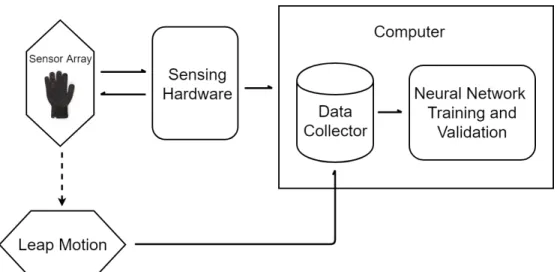
3-1 A high-level diagram of how all the software and hardware fit together. A sensor array is integrated on a glove and sensing hardware is used
to collect and transmit strain data from the glove to a computer. On the computer there are two big components. The data collector collects
data synchronously from the sensor array and a Leap Motion. Separate sets of data are used to train and validate a neural network. . . 25
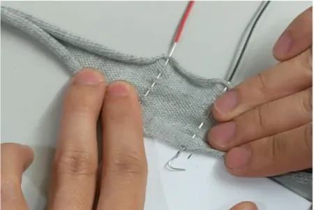
3-2 A strip of conductive knitted fabric is stretched and probed to observe
it’s strain sensing capabilities. Special thanks to Alexandre Kaspar for fabricating this sensor. . . 26
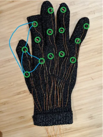
3-3 The glove was an off the self conductive glove for use with touchscreens.
Sense points were attached to 14 locations on the glove. The locations approximately matched the location of finger joints. This image shows
the wire routing (gold magnet wire) of the glove and highlights the sense points(green circles). A subset of the sensors in this array are
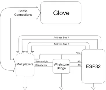
4-1 A High-Level diagram of the sensing system. The ESP32 controls the multiplexers using digital addressing buses. The multiplexers switch
which sensor on the glove is being sensed. The ESP32 reads the selected sensor through the Wheatstone bridge. More hardware diagrams can
be found in appendix b. . . 31
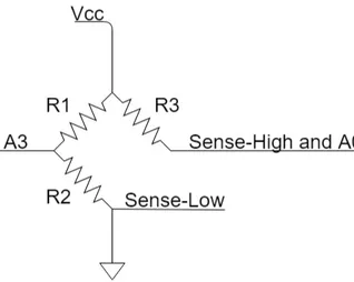
4-2 The Wheatstone bridge is a common resistance based sensing
topol-ogy. Three resistors of known resistance are connected to a variable resistance and the voltage difference between the center legs can be
used to calculate the value of the variable resistor. . . 32
4-3 The multiplexer system block consists of two analog mux boards. These each mux has 4 addressing pins which allows it to connect a sense pin to
one of 14 sensor nodes on the glove. One mux is denoted the high mux because it’s sense line is attached to the high leg of the Wheatstone
bridge while the low mux is connected to the low leg of the Wheatstone bridge. Note that ch0 of mux_h connects to ch0 mux_l and the first
sensing node on the glove. . . 34
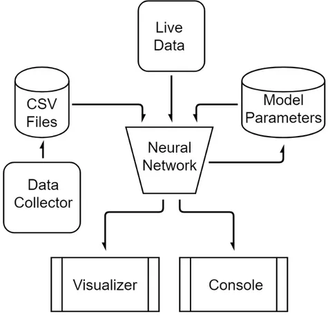
5-1 A diagram of the entire software system. . . 37
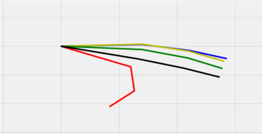
5-2 The hand visualizer shows fingers in the y-z plane relative to the hand.
The thumb is the black. The index finger is red. The middle finger is green, the ring finger is yellow, and the pinky is blue. . . 40
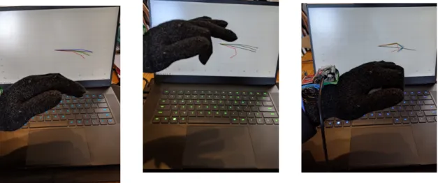
5-3 Hand poses matched by Visualizer . . . 41
6-1 Simultaneous collection of data from the Leap Motion and glove. Here a Leap Motion visualizer is shown on the right and a sample count on
the left. The Leap Motion had some error in it’s own measurement so it was important to watch the visualization as data was being collected. 44
6-2 Several hand positions being detected as the same hand position by
B-1 The initial prototype of the glove. This glove uses conductive thread insulated with electrical tape to connect various points to the
multi-plexers on the bread board . . . 53 B-2 The second prototype of the glove. This glove uses magnet wire to
connect to the multiplexers on the protoboard. The magnet wire is sewn under the glove to keep it hidden. . . 54
B-3 A schematic diagram of the sensing hardware that was built. Note that all 14 connections between the the multiplexers (left) each lead to
a sensing node on the glove. There is a wheatstone bridge (top right) and an ESP32 devboard (right) . . . 55
B-4 An illustration of how the sensing hardware was wired. Note that all 14 connections between the the multiplexers (left) each lead to a sensing
node on the glove. There is a wheatstone bridge (top right) and an ESP32 devboard (right) . . . 55
List of Tables
Chapter 1
Technical Approach to Sensorized
Textiles
E-textile sensors have extensive applications in health monitoring, entertainment, and sports training. Since these sensors can be integrated directly into clothing, a
lot of data can be tracked. Sensors that track sleep, body temperature, and heart rate could help monitor human health and suggest habit corrections. Sensors could
be used to track body language. This data could be used to identify environmental sources of stress. This work presents a novel technique for strain sensor using e-textiles
integration. This technique is both low-cost and easy to fabricate. The technique is applied to a glove to create a hand position tracking glove, and the glove is evaluated
against previous works.
The sensing technique is applied to hand position tracking because hand position
tracking can be applied to many applications. For example, hand tracking can be used to track and encourage daily hand exercises for physical therapy. Hand posture
could be tracked while typing and suggest changes to prevent long term injury. Hand gesture recognition is another possibility which would lead various human computer
interfaces. Sign language interpretation is also a possibility.
Hand position tracking with a glove presents several challenges. Sensors need to be small to fit on the fingers. Additionally, there must be enough sensors to capture
requires dense layouts of sensors and complex wire routing.
There have been several previous attempts to create a hand position tracking
glove as seen in the following works [3, 2, 14, 12, 6, 4, 8, 13]. These gloves all use different approaches to achieve hand position tracking. The methods of fabrication
all vary, but they are all still fairly involved processes. Some require polymer casting and component embedment [2, 4]. Others require fabrication of a flexible sheet of
sensing material followed by laser cutting [6, 3].
In this work a hand position tracking glove that can be fabricated with simple
workbench tools and low cost materials. The solution presented here involves making 𝑁 wired connections to a commercially available touch screen glove. Using
funda-mental ideas from [11, 14], it can be seen that resistances measured between any two nodes will relate to the strain between those nodes. Thus a sensor array is integrated
into the glove and the number of sensors in the array is(︀𝑁2)︀. Then a neural network is trained to predict hand positions based on the readings provided by the sensor array
to demonstrate the performance of this method.
1.1
Contributions
For this work, a strain sensing glove prototype was built and tested. The design was
iterated on to reduce the form factor. An embedded multiplexed sensing system was developed to read and transmit data to a computer in a synchronized manner. A
Python script was developed to collect synchronized data from the glove and a Leap Motion, which was posing as the ground truth in training the neural network.
An-other Python script was developed to train the neural network, test the network on a chosen data set, and perform a live 2D visualization of hand pose predictions given
sensor readings form the serial port. Credit for the initial development of the neural network goes to Andrew Spielberg.
This thesis contributes:
∙ A machine learning algorithm for extracting hand pose and activity from the senorized glove
∙ A 2D hand pose visualizer ∙ Experiments and evaluations
1.2
Outline
Chapter 1 introduces the motivation behind this work. The problem of sensor inte-gration and the proposed solution is presented.
Chapter 2 is a literature review that covers topics which are critical to under-standing material presented in the rest of the work. This chapter also differentiates
techniques used in this work from techniques developed in previous works.
Chapter 3 describes the system implemented as a whole. There is a high-level
explanation of what each module does. Then there is a description of how training and test data was collected for the Neural Network.
Chapter 4 covers the implementation of hardware. There are detailed descriptions of how each hardware module works, and then there is a section on how parts were
selected.
Chapter 5 explains the implementation of software. There is a description of the
neural network architecture and it’s learning rate. The format data input and output is stated. Finally, there is an description of the visualizer.
Chapter 6 the presents the results of the glove. Evaluation metrics are defined and the performance of the glove is discussed.
Chapter 7 concludes the work. There is a reflection of what was learned and how the system could be improved in a future iteration. Additionally, some future works
Chapter 2
Literature Review
There have been several past works on hand position tracking gloves. To differentiate
all these works it is necessary to formulate a classification for the techniques used. This will also provide a way to describe where this work fits in the grand scheme
of things. To start, a review be Castano and Flatau presents a way to classify vari-ous sensing techniques into two broad categories [1]. There are techniques that use
extrinsic modification of textiles to achieve smart sensing and there are techniques that use intrinsic modification of textiles to achieve smart sensing. Several gloves
that incorporate extrinsic modification are presented in this review by Rashid and Hasan [13]. Each of the gloves have some kind of pre-made sensor attached to it to
achieve smart sensing. Gloves that incorporate intrinsic modification of textiles are seen in work by Glauser and work by Ryu [3, 14]. These gloves use some property of
the fabric to build sensors. The glove presented in this work uses intrinsic sensing to achieve hand position tracking.
2.1
Fabric Structures
The structure of a fabric sensor often times plays a critical role in how the sensor
responds to stimuli. For this reason it is important to establish an understanding of fabric structures at a low level before diving into the physics behind sensors. Fabric
many sub classifications.
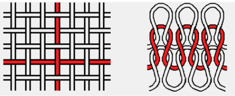
Figure 2-1: A comparison of a woven structure (left) and knit structure (right). This figure was taken from Alexandre Kaspar’s introduction to machine knitting web page.
Figure 2-1 shows the differences between woven and knit fabrics. Woven fabrics
are composed of many strands of material which are interleaved with perpendicular strands. The knit fabric is composed of yarn that is looped into the loops of yarn in
the previous row. In knit fabrics, the rows here are called courses and the columns are called wales. It is worth noting that the first and last course of a knit fabric are
knit in a way that prevents the fabric from coming apart under tension. There are various knitting techniques that can change the fabric structure as seen in work by
McCann and work by Narayanan [9, 7]. This work only requires knowledge of the basic knit structure presented.
2.2
Sensing Mechanisms
Intrinsic sensing mechanisms can be classified as one of three types, resistive,
capaci-tive, and inductive. All of these work on the similar principles. The signal of interest is coupled to the resistance, capacitance, or inductance of the sensor, and the changes
in impedance are measurable.
Capacitance based strain sensors require two conductive sheets of fabric to act as electrodes. In research done by Atalay, a conductive fabric is attached to a silicon
elastomer. The fabric and elastomer are then laser cut to create two adjacent con-ductive patches or electrodes. Then the device is encased in more silicon elastomer
move closer together which increases capacitance [10].
Inductive based sensing was explored in work by Koo. In this work, a coil made of conductive yarn was embroidered into a jacket. The idea here was that by injecting
a current into the coil, a magnetic field would be produced which would be coupled to the impedance of the human body. The magnetic field would induce measurable
eddy currents back into the coil which were related to blood flow and breathing [5].
Another work by Atalay tested the performance of resistance based knit sensors. A composite knit was made with alternating courses of conductive yarns and
non-conductive elastomeric yarns. Self contact in the non-conductive courses would vary with stretching thus changing the resistance [11].
2.3
Techniques Used in Previous Works
There are a plethora of techniques used to track hand positions. These techniques
are not limited to gloves. This section will present various techniques used for hand tracking and discuss the pros and cons of each method.
2.3.1
Camera-Based Hand Tracking
Commercial products such as Motion Capture and Leap Motion are examples of camera based hand tracking. Motion Capture is a marker based tracking system
which uses several cameras to reconstruct the 3D position of markers. There is also propriety software available for the specific task of tracking hand and body motions.
Leap Motion uses an IR camera and transmitter to detect hands in the work space of the camera. There is also active research on camera-based hand tracking. Work
by Taylor demonstrates hand tracking method using a depth camera [15]. These techniques have been shown to have high accuracy, but are often limited in mobility
2.3.2
Microfluidic Strain Sensing
Work by Chossat presents a silicone cast sensing glove [2]. The glove has a conductive fluid embedded into microfluidic channels along the glove. Stretching changes the
resistance of the measured in the channels. Work by Hammond is another example in which modular sensors that can be easily integrated [4]. These gloves show promising
results, but their fabrication methods are relatively complex.
2.3.3
Capacitive Strain Sensing
A recent paper by Glausser shows a lot of promise as an accurate sensing glove [3]. This glove utilizes ideas from Atalay [10]. The idea of a data driven glove is also
presented here. This work claims a simple fabrication process. While this process is relatively simple compared to the microfluidic sensing, it still requires several steps
and some tools only available in modern fab labs. It is worth noting that capacitive sensing is highly linear with no hysteresis though. These are qualities that do not
carry over to resistive strain sensing.
2.3.4
Resistive Strain Sensing
The gloves presented in Lorussi and in Ryu use resistive strain based sensing [6, 14]. This work is most similar to the work by Ryu. The sensing is based on the changes in
resistance in a conductive knit structure. The main difference is how the sensors are integrated. In Ryu, a small patch of conductive material is wrapped around fingers
at points of interest and the material is probed. In the work, there is no addition of knitted material. Wires are directly connected to the glove which reduces the
fabrication time.
2.4
Selecting a Sensing Mechanism
In the brainstorming stage of this work, one goal was to find a unique way to apply
hand rehabilitation showed an abundance of sensing gloves that had been built [13]. One thing that all the gloves had in common was the need to attach the external
sensors to the glove. With the knit sensors it would be possible to make the sensors a part of the glove itself. To integrate the sensor into the glove, the sensing mechanism
would have to be very minimal. Resistive sensing was chosen because it was the only mechanism which naturally took advantage of the physical structure of the fabric.
2.4.1
Applying Resistance Based Sensing
Consider the effects of making a knitted fabric from a strand of conductive yarn. The fabric would have some measurable resistance associated with it. Atalay’s work
on resistive knit strain senors identifies two factors that contribute to the resistance of the fabric. The yarn itself has a length-wise resistance. This resistance can be
modeled with the following equation:
𝑅 = 𝜌𝑙 𝐴
Where 𝜌 is the resistivity, 𝑙 is the length and 𝐴 is the cross sectional area of the yarn. If the yarn is stretched there would be an increase in resistance because
the length would increase and the cross sectional area would decrease assuming a positive Poisson ratio. The second factor has to do with contact resistance due to self
contact within the knitted structure. In the knit structure, the conductive yarn can contact itself which can create a lower resistance path for conduction thus reducing
the resistance. This contact resistance is modeled with the following equation which is based on Holm’s contact theory.
𝑅𝑐 = 𝜌 2 √︂ 𝜋𝐻 𝑛𝑃
Here 𝜌 is still the resistivity, 𝐻 material hardness, 𝑛 is the number of contact points and 𝑃 is the contact pressure. In this work every course is conductive, thus conduction
structure, stretching the fabric causes the loops to pull and push on each other. This increases the number of contact points and contact pressure thus reducing the
resistance at self contacts. Assuming the contacts have lower resistance than the length-wise resistance, the overall resistance of the fabric will decrease.
Chapter 3
System Overview
We have developed a novel slenderized glove device and supporting software system for tracking the human activity through the sensors embedded in the textile of the
glove.
Figure 3-1: A high-level diagram of how all the software and hardware fit together. A sensor array is integrated on a glove and sensing hardware is used to collect and transmit strain data from the glove to a computer. On the computer there are two big components. The data collector collects data synchronously from the sensor array and a Leap Motion. Separate sets of data are used to train and validate a neural network.
The system here proposes a data driven method for achieving hand position track-ing. Figure 3-1 shows a basic overview of how various components are connected. A
a skeletal hand model with 45 DoFs. The hand model is described in further detail in Chapter 5.
3.1
Theory of Operation
A Shima Seki knitting machine was initially used to knit a strip of fabric using conduc-tive steel coated yarn. The knitting pattern was a basic uniform knit pattern. This
strip was used to initially test the viability of strain sensing with knitted conductive fabric. This was the first attempt to emulate the sensing mechanism described in
work by Atalay [11].
Figure 3-2: A strip of conductive knitted fabric is stretched and probed to observe it’s strain sensing capabilities. Special thanks to Alexandre Kaspar for fabricating this sensor.
The probes were connected to a voltage divider circuit that was provided 3.3 Volts. The voltage was measured on an oscilloscope. The measured change in voltage was
about 250 mV for about a stretch of .25 inches. This stretching is on the order of what would be expected in a glove, and the voltage range is reasonably large. 250
mV translates to 310 representable values from a 12 bit Analog to Digital Converter (ADC). Once the sensing mechanism was verified as a viable solution, we wanted
had previously designed an fabricated gloves on the Shima Seki, but due to limited quantities of conductive yarn, it was not viable to make a glove. Thus a standard
touch screen glove was purchased and tested. The testing of the glove is described in Chapter 4.
The glove was made of a silver conductive yarn and a non conductive polyester yarn. It had the same basic knit structure as the strip of conductive yarn that was
initially tested. There were 14 sensing points made on the glove. Between those 14 points there were 91 total unique pairs of sensing points. Each unique pair of points
was treated as a sensor in the sensor array.
Figure 3-3: The glove was an off the self conductive glove for use with touchscreens. Sense points were attached to 14 locations on the glove. The locations approximately matched the location of finger joints. This image shows the wire routing (gold magnet wire) of the glove and highlights the sense points(green circles). A subset of the sensors in this array are also loosely illustrated here (blue curves).
There were two main options to measure readings from the 91 sensors. One option
unique ADC pin on the microcontroller (ESP32). One big drawback to this approach was that the ESP32 doesn’t have 91 ADC pins. In fact it is not very common for
any prototyping board to have 91 ADC pins. As a result a time multiplexing solution was developed. Two analog muxes would control which sense points were connected
to a Wheatstone bridge sensing circuit. The microcontroller could then sequentially select different sensors from the array and read their values in time. This approach
only requires one sensing circuit and one ADC. It is limited by the time it takes to sample each sensor and the number of sensors per sample. This is discussed in the
multiplexing section below.
These sensor readings provide information related to the position of the hand. The hand model has 45 DoFs. Given the nature of the sensing array, it is clear
that not all the sensors are independent. To understand this, consider three nodes 𝑁1, 𝑁2, 𝑁3. These nodes have three edges representing the resistances between each
node. Consider a configuration in which these nodes are placed in a vertical line such that 𝑁1 and 𝑁3 are above and below 𝑁2 respectively. Assume resistance measured
is based on the distance between two nodes. It is clear that the resistance between 𝑁1 and 𝑁3 is equivalent to a sum of resistance between node 𝑁1 to 𝑁2 and 𝑁2 to
𝑁3. The result here is that any edge which is a spatial series combination of other edges on the glove is not independent. It was determined that there is a conservative
count of 13 independent sensor readings. This count does not consider the effects of self contact between fingers. Since the conservative count is less than the number
of DoFs it is possible that there is not enough sensor data to accurately determine the hand position. As a counter to this point, the motions of the hand are not fully
independent. For example, it is very difficult to bend the tip of any finger without bending the middle joint as well. Subtle dependencies in hand motions reduce the
true DoFs. This will be discussed further in Chapter 6.
The sensor readings are provided to a neural network either in a pre-made data
set or live via serial communication. The pre-made data sets are captured using a data collection script. Data sets are collected for either training or testing. The
this because the script will overwrite any file with the same name. The scripts for training and validation require specification of a data set to be used, whether training
or validation will be done, and a specification of the file in which the model is to be saved or loaded from.
Chapter 4
Hardware Implementation
Figure 4-1: A High-Level diagram of the sensing system. The ESP32 controls the mul-tiplexers using digital addressing buses. The mulmul-tiplexers switch which sensor on the glove is being sensed. The ESP32 reads the selected sensor through the Wheatstone bridge. More hardware diagrams can be found in appendix b.
The sensing glove was a touchscreen glove purchased from Amazon. This glove
was made by Aglove. The glove is composed of a silver conductive yarn and a non conducting acrylic fibers. The glove is knit and there is conductive yarn in all the
courses and wales. This makes the glove ideal for resistive strain sensing. As an initial test of the glove’s resistive sensing, two probes were attached to the glove
read out was around 50 Ohms. Upon stretching, this decreased to 20 Ohms. The higher resistance measured was around 100 Ohms. It was important to know the
range of resistances that could show up because the sensitivity of the Wheatstone bridge decreases as resistances get further from some calibrated resistance. Since the
fluctuations were relatively small, it was decided that there was no need for more than one Wheatstone bridge calibrated to 100 Ohms. It is also important to note the
order of the connections from the glove to the multiplexer because this determines the order of inputs given to the neural network. Starting at the thumb, the node
connected to the joint closest to the wrist is connected to ch0, then the next node up on the thumb is connected to ch1. This pattern is followed through the index,
middle, ring, and pinky fingers.
The multiplexers were chosen as easily accessible parts. Their form factor also fit
a breadboard. This reduced the complexity of the initial prototyping process. An ESP32 was chosen as the main controller for the hardware sensing because of its easy
to program and has wireless capabilities that could be easily utilized in future works.
4.1
Wheatstone Bridge
Figure 4-2: The Wheatstone bridge is a common resistance based sensing topology. Three resistors of known resistance are connected to a variable resistance and the voltage difference between the center legs can be used to calculate the value of the variable resistor.
The Wheatstone bridge is a resistor topology which is often used for resistance based sensing. The figure above shows a schematic of a standard Wheatstone bridge. 𝑅1 and 𝑅2 form a fixed voltage divider. 𝑅3 and the selected glove sensor form a
variable voltage divider. Given the fixed value resistances it is possible to calculate
the resistance of the sensor. This topology was chosen because it is more noise immune than a simple voltage divider. In addition to measuring the variable resistor leg, the
Wheatstone bridge also senses measures the voltage at of a fixed voltage divider. This allows for some corrections to sensing error due to disturbances such as fluctuations
in 𝑉𝑐𝑐. 𝑉𝑓 𝑖𝑥𝑒𝑑 = 𝑉 (𝐴3) (4.1) 𝑉𝑣𝑎𝑟𝑖𝑎𝑏𝑙𝑒 = 𝑉 (𝐴0) (4.2) 𝑉𝑑𝑖𝑓 𝑓 = 𝑉𝑣𝑎𝑟𝑖𝑎𝑏𝑙𝑒− 𝑉𝑓 𝑖𝑥𝑒𝑑 (4.3) 𝑅𝑠𝑒𝑛𝑠𝑜𝑟 = 𝑉𝑐𝑐𝑅2+ 𝑉𝑑𝑖𝑓 𝑓(𝑅2 + 𝑅1) 𝑉𝑐𝑐𝑅1− 𝑉𝑑𝑖𝑓 𝑓(𝑅2+ 𝑅1) 𝑅3 (4.4)
Equation 2.4 shows the equation used to obtain the sensor resistance from analog reads on 𝐴0 and 𝐴3. This equation is derived from basic circuit analysis of the circuit
in figure 4-2.
In this hardware implementation, two analog ports of the ESP32 are attached to
the static resistor branch and the variable resistor branch. Upon sampling a specific sensor, the ESP32 reads in the analog voltages at the ports using a 12 bit ADC. These
values are converted to volts and equation 4.3 and 4.4 are applied. All variables that are not 𝑉𝑑𝑖𝑓 𝑓 are constants that are stored in the program memory.
4.2
Multiplexer
The multiplexing reduces the amount of sensing hardware required by acting as a
sensor selection mechanism. Only one Wheatstone bridge and two ADCs a necessary for sensing in this case. This reduction in hardware is traded for an increase in
Figure 4-3: The multiplexer system block consists of two analog mux boards. These each mux has 4 addressing pins which allows it to connect a sense pin to one of 14 sensor nodes on the glove. One mux is denoted the high mux because it’s sense line is attached to the high leg of the Wheatstone bridge while the low mux is connected to the low leg of the Wheatstone bridge. Note that ch0 of mux_h connects to ch0 mux_l and the first sensing node on the glove.
a fast enough sampling rate to capture human motion. One sample from the glove consists of 91 multiplexed sensor readings. The sampling bandwidth of the ADC is
10000 samples per second, and multiplexer switching is on the order of nanoseconds. This means each sensor reading is bottle necked by analog reads done by the ADC.
Two analog reads are required per sensor reading. This means that one full sample of all the sensors requires 18.2 milliseconds. This is much faster than any motion
articulated by the human hand. It should also be noted that the multiplexers add an extra 200 Ohms of resistance in series with the glove sensors. This is not ideal
because this reduces the sensitivity of the sensors. This can be seen by analyzing how this effects the variable voltage divider leg of the Wheatstone bridge.
Using equation 4.7, we can derive the expected voltage swing given some range of
resistance on 𝑅2. Considering the non ideal case, 𝑅2 ranges from 250 Ohms to 220 Ohms this is the expected initial strain and final strain resistance plus the 200 Ohm
The following equations define in a basic voltage divider. The voltage divider consists of two resistors 𝑅1 and 𝑅2 that are in series. 𝑅1is a static resistor and 𝑅2is a variable resistor. 𝑉𝑐𝑐 is the voltage across 𝑅1 and 𝑅2. 𝑉𝑠𝑒𝑛𝑠𝑒 is the output of which changes based on changes in the variable resistance 𝑅2
𝑉𝑐𝑐 = 3.3𝑉 (4.5) 𝑅1 = 100Ω (4.6) 𝑉𝑠𝑒𝑛𝑠𝑒 = 𝑅2 𝑅1+ 𝑅2 𝑉𝑐𝑐 (4.7)
So there is a total voltage range of 90 mV. The ESP32 has an 12 bit ADC so this translates to 111 possible distinct readings that can represent the range. Now consider
the case without the resistance offset. 𝑅2 ranges from 50 Ohms to 20 Ohms. The voltage outputs of these two values is 1.1 V to 550 mV. That is a voltage swing of
550 mV. This is 682 possible distinct readings that can represent the range. Thus the added resistance of the multiplexers decreases the sensing resolution by a factor of 6.
In future implementations, it would be advised to find multiplexers with lower series resistance. Note that it would still be important to consider the switching speed as
Chapter 5
Software Implementation
Figure 5-1: A diagram of the entire software system.
The goal of the software was to develop a data driven method to predict the states
defined by our hand model using our strain sensor data. The hand model is meant to be a means of representing tracked hand positions. The software is divided into
script contains a live data collector, Neural Network, and a hand pose visualizer. The Neural Network takes in data from either a CSV file or live data and predicts outputs
based on the hand model used in this work. The hand model is based on the skeletal model that the Leap Motion produces. The Leap Motion skeletal hand model gives
each hand 5 fingers each with 4 bones. Each bone is treated as a cylinder with some initial (x, y, z) position and direction in reference to absolute coordinates. This gives
a total of 120 DoFs with no consideration to joint constraints. The coordinate system is transformed to be in reference with the hand because the glove is not intended to
track articulations beyond the hand. In this reference frame one bone in every finger is static, meaning their position and directions are independent of hand articulations.
These static bones are the bones closest to the wrist in the Leap Motion’s skeletal hand model, and they are not considered in the hand model used in this work. Additionally,
the positions of the bones only retain a sense length of finger bones. These are also removed from the hand model. This leaves x, y, and z directions for 15 bones in
reference to the hand. This gives us 45 degrees of freedom.
5.1
Neural Network Architecture
A neural net model with 4 hidden layers and 64 perceptrons per layer was built
using TensorFlow version 1.10.0. During training, a data set of 15000 samples was randomized so that the samples were not in chronological order. Half of the samples
were used to train the model while the other half was used to validate that the training
wasn’t over fitting to the training set. On each training step the model would predict a state for every DoF in the hand model for every sample in the training set. Every
sample had some error on each state. This was the difference between the expected state and the predicted state. Then the L2 norms of errors of each state is is calculated
and these aggregate values are summed together to represent the loss.
Then an Adam optimizer is used to minimize the loss. Then the loss on the test set is calculated and there is a check to see if the losses have hit a new minimum. If
The following equations show how the loss is calculated. The Predictions matrix has 45 columns and 15000 rows. Each row represents a predicted output for each input given to the neural network. Each individual 𝑝𝑖𝑗 represents a predicted value assigned to the jth DoF of the ith prediction. The Expected matrix has the same dimensions as the Prediction matrix. The only difference is that the individual 𝑦𝑖𝑗 represent the actual value that was captured by the Leap Motion for the jth DoF of the ith sample. The Error matrix is the element-wise difference between the Predictions matrix and the Expected matrix. 𝐿2𝑒𝑟𝑟𝑜𝑟 is a row vector with 45 columns. Each column is the L2 norm of the corresponding column in the Error matrix. loss is calculated as the sum of all the elements in the 𝐿2𝑒𝑟𝑟𝑜𝑟 vector.
Predictions = ⎡ ⎢ ⎣ 𝑝11 𝑝12 · · · 𝑝21 . .. .. . ⎤ ⎥ ⎦Expected = ⎡ ⎢ ⎣ 𝑦11 𝑦12 · · · 𝑦21 . .. .. . ⎤ ⎥ ⎦ (5.1)
Error = Predictions − Expected (5.2)
𝐿2𝑒𝑟𝑟𝑜𝑟 =[︀||𝑒𝑟𝑟𝑜𝑟1|| ||𝑒𝑟𝑟𝑜𝑟2|| · · · ]︀
(5.3)
loss =∑︁𝐿2𝑒𝑟𝑟𝑜𝑟 (5.4)
later use. Finally, the training step ends and the process is iterated. The math below shows the calculation of loss.
During testing, a model is loaded and data from a test set is loaded. The model makes predictions given input data from the test set and the hand model data is
transformed into joint angle data. This data is in a 2D plane that shows a side view of the hand. This plane was chosen because it captures finger flexion which has the
largest range of motion. The predicted angles of each joint are subtracted from the expected angles of each joint and averaged to find the average joint error. This is
used as a evaluation metric in Chapter 6.
5.2
Data Input and Output
The neural network expects 91 inputs. These inputs correspond to the sensor readings from the glove. The outputs match the 45 DoFs of the hand model that was derived
5.3
Visualization
A script was developed to feed live sensor readings into the model to predict finger positions. A visualizer was created using Python’s matlibplot library. The visualizer
is a live plot that plots fingers starting at the origin. To reduce jitter, a filter of the following form was added.
Output = 𝛼(new_prediction) + (1 − 𝛼)(Output)
𝛼 is between 0 and 1. This filter prevents very large deviations to occur from the
previous step to the next. This is reasonable considering, that human fingers can’t instantly move from one location to another. Since the data output of the model is
in 3D space it is possible to create a 3D visualization however 2D was chosen simply for demonstration purposes.
Figure 5-2: The hand visualizer shows fingers in the y-z plane relative to the hand. The thumb is the black. The index finger is red. The middle finger is green, the ring finger is yellow, and the pinky is blue.
After observing the behavior of the visualizer, it seems clear that a larger data
set is required to obtain clear hand articulations. The visualizer had a hard time differentiating the ring finger and the pinky. If the pinky was curled, then the model
would automatically curl the ring finger a bit. This could be a result of not collecting data on a hand position in which the pinky was bent and the ring finger was kept
Chapter 6
Results
The results of this work will cover some evaluation metrics. There will also be dis-cussion on some observations made during testing.
6.1
Evaluation Metrics
The overall goal of this project was meant to test and demonstrate the use of a novel knitted strain sensor array. One of the claims for this work was that the sensing array
would be low cost and easy to make. Thus tools used, fabrication time and cost are some metrics that should be evaluated. Additionally, it is important to analyze the
sensor array’s performance for hand position tracking. This metric shows the viability of this sensor array when compared to state of the art sensors. The performance of
the glove can be broken down into the amount of time required to collect all the data for training and testing, the amount of time required to train and the average error
of the glove’s predictions.
6.2
Data Collection
Data was collected simultaneously from the glove and Leap Motion using a Python script. The data sets were saved as csv files. Each row was a new sample and each
Figure 6-1: Simultaneous collection of data from the Leap Motion and glove. Here a Leap Motion visualizer is shown on the right and a sample count on the left. The Leap Motion had some error in it’s own measurement so it was important to watch the visualization as data was being collected.
inputs. The outputs were 120 values recorded from a Leap Motion. These data points were x, y, z coordinates and directions for each bone in the Leap Motion’s skeletal
hand model. The data was reduced to 45 columns to match the 45 DoFs of the hand model as described in Chapter 5. The input set was composed of 91 columns of data;
one for each sensor reading. A local averaging filter of window size 10 was applied to each of these sensor reading columns to filter out high frequency noise. Each data set
consisted of around 15000 data points. Data sets were saved as either training data or testing data to keep track of which sets had been used to train models.
As shown in figure 6-1, data was collected while watching the Leap Motion
vi-sualizer to ensure clean data was collected. Figure 6-2 shows how the Leap Motion could misinterpret hand positions. Misinterpretation of hand position from the Leap
Motion’s end would lead to improper training. These misinterpretations were avoided for the most part but a few samples of misinterpreted data did manage to get into
Figure 6-2: Several hand positions being detected as the same hand position by the Leap Motion
6.3
Performance
In terms of cost and fabrication, the sensor array was excellent. The total cost of all the hardware components was approximately $50. The glove was $14, each
multiplexer was $5.50, the ESP32 was $11 and all the wires and resistors were likely just a few cents, but I left a buffer of $14.00 in case there was another part that
was not considered. For comparison, a Leap Motion controller is $80 and other commercially available hand tracking gloves are a few hundred dollars. The tools
used were a soldering iron and solder to solder parts to the protoboard, wire strippers to cut wires to length, a multimeter to check connections, hot glue to insulate solder
connections, and sand paper to sand off the enamel on the magnet wire. All of this equipment is very affordable and is considered general work bench equipment. The
fabrication time was roughly 3 hours of work. Two hours were spent soldering and hot gluing over connections on a protoboard, and one hour was spent sanding enamel
off of magnet wire and weaving it into the glove. It is worth noting that the initial prototype took much longer to fabricate because the design wasn’t as streamlined.
To collect data, the glove was worn with an insulating glove separating the skin
from the conductive surface. The insulation was added to avoid direct contact of electronics with skin. Several hand poses were recorded over a period of 34 minutes.
as some set of fingers curled and some set of fingers uncurled. Two data sets were captured in the 34 minutes. It took 17 minutes to collect a training data set of 15000
points and 17 minutes to collect the testing data set of 15000 points.
The training was done as described in Chapter 5 using the training data set. The training took 9 minutes and ended with a test loss of 4496. The average angle error
of each joint in the training set was around 6 degrees, but since some set of the data was used to train the model this is not a good metric for overall glove accuracy.
Instead, average angle error is calculated using the test data set which was never trained on to determine accuracy of predictions. The average angle error across the
hand was 17.12 degrees for all 15000 samples that were recorded in the test set. This measure is sufficient as a measure of accuracy because no sample in the test set have
been trained on. With 15000 samples of various hand poses, the test set should be sufficient in validating an average error of the glove over several hand poses. This is
higher than all the gloves presented in the work by Glausser [3]. To compare, Glausser mentions that two gloves that were purchased had an average error of 11.93 degrees
and 10.47 degrees. The glove they made only had 6.76 degrees of error. One note for the performance of our glove is that the error in angle increases for bones that
are further from the wrist. This suggests that there is potentially some bias in the learning that causes the model to minimize error near the wrist, or that the sensor
array truly does not provide enough data to capture all the DoFs of the hand.
6.4
Disscussion
The results from the visualizer are very promising. It is clear that the sensing method that was developed definitely works. There are some potential sources of error that
should be analyzed. For one, it would likely help to find muxes with lower resistance. The muxes add a total offset resistance of about 200 Ohms. The sensors in the glove
have resistances of 50-100 Ohms. Another potential issue could be response of the glove sensors. While it was observed that the gloves detect changes in resistance
the original selection of resistors for the Wheatstone Bridge, it was assumed that the expected resistances would be around 100 Ohms so the Wheatstone Bridge was tested
Chapter 7
Conclusion
In this work, a novel method for integrating knitted strain sensor arrays was applied to a hand position tracking glove. Sensing hardware was designed to interface with
the sensor array, and a machine learning algorithm was developed to predict hand positions based on senor readings from the sensor array.
It was seen that the machine learning algorithm was able to track hand positions
with an average error of about 17 degrees of average error in joint angles. Most of the error was accumulated in joints further from the wrist. While the accuracy of the
hand tracking was worse than the state of the art hand tracking gloves, it was seen that the glove is low-cost and easy to fabricate.
The results suggest that the sensing method used here could be applied to other motion tracking applications. It is not the most accurate, but the low cost and simple
fabrication makes this method ideal for prototyping smart sensing clothing. This sensing method could lower the barrier for exploring the capabilities of e-textiles.
The array could also be built into a sleeve for a soft robot to act as a sensor for feedback control.
It seems that the results are limited in a few ways. For one the hand model that was selected for this work was different from the one chosen in Glauser [3]. To truly
measure the performance of this glove, it would be necessary to find a transformation between the two hand models. This would make the comparison less ambiguous.
Motion was capable of capturing hand positions reasonably well, but it was visibly off at many points during data collection. This could contribute to losses in training.
7.1
Future Works
The next steps would be to develop a more streamlined way to fabricate these sensors. Perhaps the sensing nodes can be sewn in by some automated process. The glove proof
of concept should be investigated further. There are still many questions here for example, would a learning model similar to the one implemented by Glauser produce
better results? Could adding more sensing nodes or moving already existing sensing nodes produce better results? Answering these questions would further develop our
understanding of what limits the performance of the sensing method and how different design parameters effect the performance of the sensing method.
Appendix A
Tables
Table A.1: Key Components
Parts Quantity
ESP32 Devboard 1
CD74HC4067 Mux 2
Original Sport Aglove 1
Appendix B
Figures
Figure B-1: The initial prototype of the glove. This glove uses conductive thread insulated with electrical tape to connect various points to the multiplexers on the bread board
Figure B-2: The second prototype of the glove. This glove uses magnet wire to connect to the multiplexers on the protoboard. The magnet wire is sewn under the glove to keep it hidden.
Figure B-3: A schematic diagram of the sensing hardware that was built. Note that all 14 connections between the the multiplexers (left) each lead to a sensing node on the glove. There is a wheatstone bridge (top right) and an ESP32 devboard (right)
Figure B-4: An illustration of how the sensing hardware was wired. Note that all 14 connections between the the multiplexers (left) each lead to a sensing node on the glove. There is a wheatstone bridge (top right) and an ESP32 devboard (right)
Appendix C
Code Implementations
1 #d e f i n e SAMPLE_PERIOD 1 2 #d e f i n e SETTLE_PERIOD 1 3 #d e f i n e NUM_PINS 14
4 #d e f i n e NUM_PAIRS NUM_PINS* (NUM_PINS−1) /2 5 #d e f i n e A_HIGH A3 6 #d e f i n e A_LOW A0 7 #d e f i n e CAL_ITERS 1 0 0 0 . 0 8 #d e f i n e PRINT_PERIOD 10 9 10 // −−−− D e c l a r e H e l p e r F u n c t i o n s 11 // Mux c l a s s 12 c l a s s Mux { 13 i n t addr [ 4 ] ; 14 p u b l i c: 15 Mux(i n t p1 ,i n t p2 ,i n t p3 ,i n t p4 ) ; 16 v o i d d i g S e l (i n t p i n ) ; 17 } ; 18 // Record Sample f u n c t i o n 19 d o u b l e r e c o r d _ s a m p l e (i n t p_a , i n t p_b) ; 20 v o i d c a l i b r a t e ( ) ; 21 22 // −−−− Setup Muxing 23 // High S i d e P i n s 24 i n t mHs0 = 2 ;
25 i n t mHs1 = 0 ; 26 i n t mHs2 = 4 ; 27 i n t mHs3 = 1 6 ; 28 // Low S i d e P i n s 29 i n t mLs0 = 1 9 ; 30 i n t mLs1 = 1 8 ; 31 i n t mLs2 = 5 ; 32 i n t mLs3 = 1 7 ; 33 34 //Mux C l a s s o b j e c t s 35 Mux m_H( mHs0 , mHs1 , mHs2 , mHs3 ) ; 36 Mux m_L( mLs0 , mLs1 , mLs2 , mLs3 ) ; 37 38 // −−−− S e t up g l o b a l v a r i a b l e s 39 c h a r o u t p u t [ 2 0 0 0 ] ; 40 i n t p a i r _ s e l = 0 ; 41 c o n s t f l o a t R1 = 1 0 9 . 4 ; 42 c o n s t f l o a t R3 = 1 1 6 . 5 ; 43 c o n s t f l o a t R2 = 1 0 9 . 4 ; 44 c o n s t d o u b l e v1 = 3 . 3 ; 45 d o u b l e R_cals [NUM_PAIRS ] ; 46 d o u b l e R_delts [NUM_PAIRS ] ; 47 48 49 l o n g l o n g s_time = m i c r o s ( ) ; 50 l o n g l o n g p_time = m i c r o s ( ) ; 51 52 v o i d s e t u p ( ) { 53 // S t a r t t h e S e r i a l Comms 54 S e r i a l . b e g i n ( 1 1 5 2 0 0 ) ; 55 d e l a y ( 1 0 0 ) ; 56 57 // S e t up P i n s 58 pinMode ( mHs0 , OUTPUT) ; 59 pinMode ( mHs1 , OUTPUT) ; 60 pinMode ( mHs2 , OUTPUT) ;
61 pinMode ( mHs3 , OUTPUT) ; 62 pinMode ( mLs0 , OUTPUT) ; 63 pinMode ( mLs1 , OUTPUT) ; 64 pinMode ( mLs2 , OUTPUT) ; 65 pinMode ( mLs3 , OUTPUT) ; 66 67 // c a l i b r a t e ( ) ; 68 // w h i l e ( ! S e r i a l . a v a i l a b l e ( ) ) {} 69 // S e r i a l . r e a d ( ) ; 70 } 71 72 v o i d l o o p ( ) { 73 i f( m i c r o s ( )−s_time > SAMPLE_PERIOD) 74 { 75 p a i r _ s e l = 0 ;
76 f o r(i n t p_a = 0 ; p_a < NUM_PINS; p_a++){
77 f o r(i n t p_b = p_a+1; p_b < NUM_PINS; p_b++){
78 R_delts [ p a i r _ s e l ] = ( r e c o r d _ s a m p l e ( p_a , p_b) − R_cals [ p a i r _ s e l
] ) ; 79 s_time = m i c r o s ( ) ; 80 p a i r _ s e l ++; 81 } 82 } 83 } 84 i f( S e r i a l . a v a i l a b l e ( ) ) { 85 S e r i a l . r e a d ( ) ; 86 i f( m i c r o s ( )−p_time > PRINT_PERIOD) { 87 88 s p r i n t f ( output ," %4.2 f ", R_delts [ 0 ] ) ; 89 f o r(i n t p a i r = 1 ; p a i r < NUM_PAIRS; p a i r ++){ 90 s p r i n t f ( o u t p u t+s t r l e n ( o u t p u t ) , " ,%4.2 f ", R_delts [ p a i r ] ) ; 91 } 92 S e r i a l . p r i n t l n ( o u t p u t ) ; 93 p_time = m i c r o s ( ) ; 94 } 95 }
96 }
Listing C.1: Sensor reading code written for the ESP32 in the Arduino IDE.
1 Mux : : Mux(i n t p1 ,i n t p2 ,i n t p3 ,i n t p4 ) { 2 // S e t t h e Mux p i n s f o r a d d r e s s i n g 3 addr [ 0 ] = p1 ; 4 addr [ 1 ] = p2 ; 5 addr [ 2 ] = p3 ; 6 addr [ 3 ] = p4 ; 7 } 8 9 v o i d Mux : : d i g S e l (i n t p i n ) {
10 // Takes i n a p i n number f o r t h e Mux t o a d d r e s s and a d d r e s s e s t h a t p i n 11 // Each p i n has an a d d r e s s composed o f i t ’ s hex r e p r e s e n t a t i o n
12 d i g i t a l W r i t e ( addr [ 0 ] , p i n & 0 x1 ) ; 13 d i g i t a l W r i t e ( addr [ 1 ] , p i n & 0 x2 ) ; 14 d i g i t a l W r i t e ( addr [ 2 ] , p i n & 0 x4 ) ; 15 d i g i t a l W r i t e ( addr [ 3 ] , p i n & 0 x8 ) ; 16 } 17 18 d o u b l e r e c o r d _ s a m p l e (i n t p_a , i n t p_b) { 19 // L o c a l v a r i a b l e s f o r math c a l c u l a t i o n s 20 d o u b l e v_p = 0 ; // V o l t a g e measured a t t h e s t a t i c v o l t a g e d i v i d e r 21 d o u b l e v_m = 0 ; // V o l t a g e measured a t t h e v a r i a b l e v o l t a g e d i v i d e r 22 d o u b l e v2 = 0 ; // C a l u l a t e d d i f f e r e n c e between t h e s t a t i c and v a r i a b l e d i v i d e r 23 d o u b l e R _ o f f s e t = 0 ; // The c a l c u l a t e d r e s i s t a n c e o f t h e v a r i a b l e r e s i s t o r 24 25 // F i r s t s e l e c t t h e Mux p i n s t o c o n n e c t . T h i s d e t e r m i n e s which n o d e s a r e b e i n g measured 26 m_H. d i g S e l ( p_a ) ; 27 m_L. d i g S e l (p_b) ; 28
29 // Wait some t i m e f o r t h e Mux t o s e t t l e from s w i t c h i n g 30 l o n g l o n g b_time = m i c r o s ( ) ;
31 w h i l e( m i c r o s ( ) − b_time < SETTLE_PERIOD) 32 {}
33 // Make a measurement and c o n v e r t from b i t depth t o v o l t a g e 34 v_p += analogRead (A_HIGH) * 3 . 3 / 4 0 9 6 . 0 ; 35 v_m += analogRead (A_LOW) * 3 . 3 / 4 0 9 6 . 0 ; 36 37 // Do Math C a l c u l a t i o n s 38 v2 = v_m − v_p ; 39 R _ o f f s e t = ( ( R2* v1+(R1+R2 ) * v2 ) / ( R1* v1 − ( R1+R2 ) * v2 ) ) *R3 ; 40 r e t u r n R _ o f f s e t ; 41 // r e t u r n v_p ; 42 // r e t u r n v_m; 43 } 44 45 v o i d c a l i b r a t e ( ) {
46 memset ( R_cals , 0 , s i z e o f(d o u b l e) *NUM_PAIRS) ; 47 f o r(i n t i = 0 ; i < CAL_ITERS ; i ++){
48 p a i r _ s e l = 0 ; 49 S e r i a l . p r i n t l n ( i ) ;
50 f o r(i n t p_a = 0 ; p_a < NUM_PINS; p_a++){
51 f o r(i n t p_b = p_a+1; p_b < NUM_PINS; p_b++){
52 w h i l e( m i c r o s ( )−s_time < SAMPLE_PERIOD − SETTLE_PERIOD | | m i l l i s
( ) <100)
53 R_cals [ p a i r _ s e l ] += r e c o r d _ s a m p l e ( p_a , p_b) /CAL_ITERS ; 54 s_time = m i c r o s ( ) ; 55 p a i r _ s e l ++; 56 } 57 } 58 } 59 // f o r ( i n t c a l = 0 ; c a l < NUM_PAIRS; c a l ++){ 60 // R_cals [ c a l ] /= CAL_ITERS ; 61 // }
62 }
Listing C.2: Helper functions for sensor reading code written for the ESP32 in the Arduino IDE.
1 i m p o r t os , s y s , i n s p e c t , time , s e r i a l
2 s r c _ d i r = o s . path . dirname ( i n s p e c t . g e t f i l e ( i n s p e c t . c u r r e n t f r a m e ( ) ) ) 3 a r c h _ d i r = ’ . . / l i b / x64 ’ i f s y s . m a x s i z e > 2**32 e l s e ’ . . / l i b / x86 ’ 4 s y s . path . i n s e r t ( 0 , o s . path . a b s p a t h ( o s . path . j o i n ( s r c _ d i r , a r c h _ d i r ) ) ) 5 s y s . path . i n s e r t ( 0 , o s . path . a b s p a t h ( o s . path . j o i n ( s r c _ d i r , ’ . . / l i b / ’) ) ) 6
7
8 i m p o r t Leap , s y s , time , d a t e t i m e
9 from Leap i m p o r t C i r c l e G e s t u r e , KeyTapGesture , ScreenTapGesture ,
S w i p e G e s t u r e
10
11 c l a s s S a m p l e L i s t e n e r ( Leap . L i s t e n e r ) :
12 f i n g e r _ n a m e s = [’Thumb ’, ’ I n d e x ’, ’ Middle ’, ’ Ring ’, ’ Pinky ’] 13 bone_names = [ ’ M e t a c a r p a l ’, ’ P r o x i m a l ’, ’ I n t e r m e d i a t e ’, ’ D i s t a l ’] 14 #state_names = [ ’ STATE_INVALID ’ , ’STATE_START ’ , ’STATE_UPDATE ’ , ’
STATE_END ’ ]
15 p a s t = d a t e t i m e . d a t e t i m e . now ( ) 16 timed = 0
17 sample_count = 0 18 g l o v e _ d a t a = ’ ’
19 f= open(" . / Desktop / Test_data_5_17_set1 . c s v ","w+") 20 s e r = s e r i a l . S e r i a l (’COM8 ’, 1 1 5 2 0 0 , t i m e o u t = . 0 0 1 ) 21 t i m e . s l e e p ( 1 ) 22 s e r . f l u s h I n p u t ( ) 23 24 d e f o n _ i n i t ( s e l f , c o n t r o l l e r ) : 25 p r i n t (" I n i t i a l i z e d ") 26 27 d e f on_connect ( s e l f , c o n t r o l l e r ) : 28 p r i n t (" Connected ") 29 30 d e f o n _ d i s c o n n e c t ( s e l f , c o n t r o l l e r ) :
31 # Note : n o t d i s p a t c h e d when r u n n i n g i n a d e b u g g e r . 32 p r i n t (" D i s c o n n e c t e d ") 33 34 d e f o n _ e x i t ( s e l f , c o n t r o l l e r ) : 35 p r i n t (" E x i t e d ") 36 s e l f . f . c l o s e ( ) 37 s e l f . s e r . c l o s e ( ) 38 39 d e f on_frame ( s e l f , c o n t r o l l e r ) :
40 # Get t h e most r e c e n t frame and r e p o r t some b a s i c i n f o r m a t i o n 41 s e l f . timed = ( ( d a t e t i m e . d a t e t i m e . now ( ) − s e l f . p a s t ) . m i c r o s e c o n d s ) 42 43 frame = c o n t r o l l e r . frame ( ) 44 b o n e s = [ ] 45 bone_count = 0 46
47 # Get one hand e v e r y 40 m i l l i s e c o n d s 48 i f(l e n( frame . hands ) > 0 ) :
49 hand = frame . hands [ − 1 ] # g e t t h e l a s t hand d e t e c t e d 50 # b a s i s = hand . b a s i s # f i n d t h e b a s i s o f t h e hand t o f i n d r e l a t i v e d i r e c t i o n s o f f i n g e r b o n e s 51 # x _ b a s i s = b a s i s . x _ b a s i s 52 # y _ b a s i s = b a s i s . y _ b a s i s 53 # z _ b a s i s = b a s i s . z _ b a s i s 54 # o r i g i n = b a s i s . o r i g i n 55
56 # d e c i d e which t r a n s l a t i o n makes t h e most s e n s e . 57 # t r a n s = hand . f i n g e r s [ 0 ] . bone ( 3 ) . p r e v _ j o i n t 58 # o r i g i n = hand . w r i s t _ p o s i t i o n 59 # t r a n s = hand . p a l m _ p o s i t i o n 60 hand_x_basis = hand . b a s i s . x _ b a s i s 61 hand_y_basis = hand . b a s i s . y _ b a s i s 62 hand_z_basis = hand . b a s i s . z _ b a s i s 63 h a n d _ o r i g i n = hand . p a l m _ p o s i t i o n
hand_z_basis , h a n d _ o r i g i n ) 65 hand_transform = hand_transform . r i g i d _ i n v e r s e ( ) 66 67 f o r f i n g e r i n hand . f i n g e r s : 68 # Get b o n e s 69 f o r b i n r a n g e( 0 , 4 ) : 70 bone = f i n g e r . bone ( b ) 71 j o i n t = hand_transform . t r a n s f o r m _ p o i n t ( bone . p r e v _ j o i n t ) 72 b o n e s . append ( j o i n t [ 0 ] ) 73 b o n e s . append ( j o i n t [ 1 ] ) 74 b o n e s . append ( j o i n t [ 2 ] ) 75 76 d i r e c t = hand_transform . t r a n s f o r m _ d i r e c t i o n ( bone . d i r e c t i o n ) 77 b o n e s . append ( d i r e c t [ 0 ] ) 78 b o n e s . append ( d i r e c t [ 1 ] ) 79 b o n e s . append ( d i r e c t [ 2 ] ) 80 # p r i n t ( d i r e c t [ 2 ] ) 81 # p r i n t ( " bone { } : { } , { } , { } " . f o r m a t ( b , b o n e s [ f i n g *12+3*b +0] , bones [ f i n g *12+3*b +1 ] , bones [ f i n g *12+3*b +2]) ) 82 # bone = f i n g e r . bone ( 4 ) 83 # b o n e s . append ( bone . p r e v _ j o i n t [ 0 ] − t r a n s [ 0 ] ) 84 # b o n e s . append ( bone . p r e v _ j o i n t [ 1 ] − t r a n s [ 1 ] ) 85 # b o n e s . append ( bone . p r e v _ j o i n t [ 2 ] − t r a n s [ 2 ] ) 86 s = " , " 87 # p r i n t ( s . j o i n (map( s t r , b o n e s ) ) ) 88 bones_data = s . j o i n (map(s t r , b o n e s ) ) + ’ , ’ 89 s e l f . f . w r i t e ( bones_data ) 90 91 c = ’ ’ 92 s e l f . s e r . w r i t e (’m ’) 93 s e l f . s e r . f l u s h ( ) 94 w h i l e ’ \n ’ n o t i n c : 95 c += s e l f . s e r . r e a d ( s e l f . s e r . i n W a i t i n g ( ) ) 96 g l o v e = s e l f . g l o v e _ d a t a
97 g , s e l f . g l o v e _ d a t a = c . s p l i t (’ \n ’) 98 g l o v e += g 99 s e l f . f . w r i t e ( g l o v e ) 100 # s e l f . f . w r i t e ( " \ n " ) 101 s e l f . p a s t = d a t e t i m e . d a t e t i m e . now ( ) 102 p r i n t( s e l f . sample_count ) 103 s e l f . sample_count += 1 104 105 106 107 108 d e f main ( ) : 109 # C r e a t e a sample l i s t e n e r and c o n t r o l l e r 110 l i s t e n e r = S a m p l e L i s t e n e r ( ) 111 c o n t r o l l e r = Leap . C o n t r o l l e r ( ) 112
113 # Have t h e sample l i s t e n e r r e c e i v e e v e n t s from t h e c o n t r o l l e r 114 c o n t r o l l e r . a d d _ l i s t e n e r ( l i s t e n e r ) 115 116 # Keep t h i s p r o c e s s r u n n i n g u n t i l E n t e r i s p r e s s e d 117 p r i n t (" P r e s s E n t e r t o q u i t . . . ") 118 t r y: 119 s y s . s t d i n . r e a d l i n e ( ) 120 e x c e p t K e y b o a r d I n t e r r u p t : 121 p a s s 122 f i n a l l y:
123 # Remove t h e sample l i s t e n e r when done 124 c o n t r o l l e r . r e m o v e _ l i s t e n e r ( l i s t e n e r ) 125
126
127 i f __name__ == "__main__": 128 main ( )
Listing C.3: Python 2.7 script used to collect data from the Leap Motion and glove simultaneously.
2 i m p o r t IPython 3 i m p o r t numpy a s np 4 i m p o r t t e n s o r f l o w . c o n t r i b a s t c 5 i m p o r t s y s 6 i m p o r t time , s e r i a l 7 i m p o r t m a t p l o t l i b . p y p l o t a s p l t 8 i m p o r t m a t p l o t l i b . a n i m a t i o n a s a n i m a t i o n 9 from m a t p l o t l i b i m p o r t s t y l e 10 11 np . s e t _ p r i n t o p t i o n s ( t h r e s h o l d=s y s . m a x s i z e )
12 e x p o r t _ d i r = ’C: \ \ U s e r s \\mchou\\ Desktop \\ Machine_Learning \\
g l o v e _ r e c o n s t r u c t i o n \\ s a v e d _ m o d e l _ d i r e c t i o n _ o n l y ’
13 c h e c k p t _ f i l e n a m e = ’ checkpt_rel_dir_5_17_nobase_nonorm_test ’ 14 c h e c k p t _ d i r = ’C: \ \ U s e r s \\mchou\\ Desktop \\ Machine_Learning \\
g l o v e _ r e c o n s t r u c t i o n \\ ’ + c h e c k p t _ f i l e n a m e 15# d a t a _ d i r = ’ . / Averaged_data_window_10_direction_only . c s v ’ 16 d a t a _ d i r = ’ . / Train_data_5_16_set1_direction_only_avg_nobased . c s v ’ 17# d a t a _ d i r = ’ . / Train_data_5_15_fixed_direction_only_avg_win10 . c s v ’ 18# d a t a _ d i r = ’ . / Train_data_5_16_pos_only_avg . c s v ’ 19 20 21# Data p l o t t i n g 22 s t y l e . u s e (’ f i v e t h i r t y e i g h t ’) 23 24 f i g = p l t . f i g u r e ( ) 25 ax1 = f i g . add_subplot ( 1 , 1 , 1 ) 26 27 d e f g e t _ a n g l e ( o u t p u t s , o u t p u t _ d i r ) : 28 d i r _ v e c = ( o u t p u t s [ 0 + ( output_dir −1) * 3 ] , o u t p u t s [ 1 + ( output_dir −1) * 3 ] , o u t p u t s [ 2 + ( output_dir −1) * 3 ] ) 29 t r u e _ a n g l e = np . a r c t a n 2 ( d i r _ v e c [ 1 ] , d i r _ v e c [ 2 ] ) 30 r e t u r n −t r u e _ a n g l e 31 32 d e f d i v i d e _ c h u n k s ( l , n ) : 33 f o r i i n r a n g e( 0 , l e n( l ) , n ) : 34 y i e l d l [ i : i + n ]
35
36 d e f n o r m a l i z e _ d a t a ( d a t a ) :
37 means = np . mean ( data , a x i s =0)
38 # means = np . r e s h a p e ( means , [ 1 , l e n ( means ) ] ) 39 s t d s = np . s t d ( data , a x i s =0) 40 # s t d s = np . r e s h a p e ( s t d s , [ 1 , l e n ( s t d s ) ] ) 41 d a t a = ( d a t a − means ) / s t d s 42 r e t u r n d a t a 43 44 45 c l a s s H a n d P o s e R e c o n s t r u c t i o n : 46 47 d e f __init__ ( s e l f , s e s s , hidden_layer_num =2 , h i d d e n _ l a y e r _ s i z e =64 , u s e _ r e l u=True , layer_norm=F a l s e ) : 48 s e l f . s e s s = s e s s 49 s e l f . hidden_layer_num = hidden_layer_num 50 s e l f . h i d d e n _ l a y e r _ s i z e = h i d d e n _ l a y e r _ s i z e 51 s e l f . u s e _ r e l u = u s e _ r e l u 52 s e l f . layer_norm = True 53 s e l f . name = ’ hand_model ’ 54 s e l f . min_loss = 30000 55 s e l f . a n g l e = 0 56 s e l f . t r u e _ a n g l e = 0 57
58 d e f c r e a t e _ m o d e l ( s e l f , num_inputs , num_outputs , l r =1e −3) : 59 s e l f . num_inputs = num_inputs #TODO: s e t i n load_data ? 60 s e l f . num_outputs = num_outputs
61 w i t h t f . v a r i a b l e _ s c o p e ( s e l f . name , r e u s e=t f .AUTO_REUSE) a s s c o p e : 62 s e l f .i n p u t = t f . p l a c e h o l d e r ( s h a p e =[None , num_inputs ] , name=" i n p u t "
, dtype=t f . f l o a t 3 2 )
63 s e l f .i n p u t = t f . P r i n t ( s e l f .i n p u t, [ s e l f .i n p u t] ) 64 x = s e l f .i n p u t
65 s e l f . o u t p u t = t f . p l a c e h o l d e r ( s h a p e =[None , num_outputs ] , name="
o u t p u t ", dtype=t f . f l o a t 3 2 )
66 f o r i i n r a n g e( s e l f . hidden_layer_num ) :
) )
68 i f s e l f . layer_norm :
69 x = t c . l a y e r s . layer_norm ( x , c e n t e r=True , s c a l e=True ) 70 i f s e l f . u s e _ r e l u :
71 x = t f . nn . l e a k y _ r e l u ( x , name=" r e l u " + s t r( i ) )
72 e l s e:
73 x = t f . nn . tanh ( x , name=" tanh " + s t r( i ) ) 74
75
76 x = t f . l a y e r s . d e n s e ( x , num_outputs * 2 , k e r n e l _ i n i t i a l i z e r=t f .
r a n d o m _ u n i f o r m _ i n i t i a l i z e r ( m i n v a l=−3e −3 , maxval=3e −3) , name=" l d f i n a l ")
77 s e l f . x = x
78 means_and_stds = t f . nn . tanh ( x , name=" t a n h f i n a l ") 79 s e l f . means = x [ : , : num_outputs ] 80 s e l f . s t d s = t f . exp ( x [ : , num_outputs : ] ) 81 82 ’ ’ ’ 83 s e l f . p r e d _ d i s t = t f . d i s t r i b u t i o n s . Normal ( l o c= s e l f . means , s c a l e= s e l f . s t d s ) 84 s e l f . o u t p u t = t f . P r i n t ( s e l f . output , [ s e l f . o u t p u t ] ) 85 s e l f . a l l _ l o s s e s = − t f . l o g ( s e l f . p r e d _ d i s t . prob ( s e l f . o u t p u t ) ) 86 s e l f . l o s s = t f . reduce_sum ( s e l f . a l l _ l o s s e s , a x i s =1) 87 ’ ’ ’ 88
89 s e l f . l o s s = t f . reduce_sum ( t f . l i n a l g . norm ( s e l f . means − s e l f . output ,
a x i s =0) , a x i s =0)
90 # s e l f . l o s s = t f . l i n a l g . norm ( s e l f . means − s e l f . o u t p u t ) 91 #TODO: move t o i n i t i a l i z a t i o n method ?
92 s e l f . o p t i m i z e r = t f . t r a i n . AdamOptimizer ( l e a r n i n g _ r a t e=l r ) 93 s e l f . m i n i m i z e r = s e l f . o p t i m i z e r . m i n i m i z e ( s e l f . l o s s ) 94 95 s e l f . s e s s . run ( t f . g l o b a l _ v a r i a b l e s _ i n i t i a l i z e r ( ) ) 96 s e l f . s a v e r = t f . t r a i n . S a v e r ( t f . t r a i n a b l e _ v a r i a b l e s ( ) ) 97 s e l f . a n g l e s = [ 0 , 0 , 0 , 0 , 0 , 0 , 0 , 0 , 0 , 0 , 0 , 0 , 0 , 0 , 0 ] 98 s e l f . a l p h a = . 7
99 100 d e f load_model ( s e l f ) : 101 p r i n t(’ Loading : ’ + c h e c k p t _ f i l e n a m e + ’ . . . ’) 102 t r y: 103 s e l f . s a v e r . r e s t o r e ( s e l f . s e s s , c h e c k p t _ d i r ) 104 p r i n t(" Model Loaded ") 105 r e t u r n 106 e x c e p t:
107 p r i n t(" Model Not Found")
108 r e t u r n
109
110 d e f load_data ( s e l f , f i l e _ l o c ) :
111 s e l f . d a t a = np . g e n f r o m t x t ( data_dir , dtype=’ f 8 ’, d e l i m i t e r=’ , ’) 112 # s e l f . d a t a = np . d e l e t e ( s e l f . data , 1 1 9 , 1 ) #TODO: f i g u r e o u t why
d a t a i s bad
113 # s e l f . d a t a = n o r m a l i z e _ d a t a ( s e l f . d a t a ) #TODO: keep t r a c k o f means /
s t d s
114 #TODO: why i s some t h e d a t a h e r e nan ? 115 s e l f . d a t a = np . nan_to_num ( s e l f . d a t a ) 116 # p r i n t ( s e l f . d a t a [ 0 ] ) 117 118 119 d e f t r a i n ( s e l f , max_num_steps = 5 0 0 0 , m i n i b a t c h _ s i z e = 1 0 2 4 ) : 120 121 122 np . random . s h u f f l e ( s e l f . d a t a ) #d a t a i s [ b a t c h _ s i z e , d a t a ] 123 124 data_cnt = s e l f . d a t a . s h a p e [ 0 ] 125 t r a i n _ d a t a = s e l f . d a t a [ : data_cnt // 2 ] 126 t e s t _ d a t a = s e l f . d a t a [ ( data_cnt // 2 ) : ] 127 128 129 130 #TODO: t r a i n i n g and t e s t s e t s 131 f o r i i n r a n g e( max_num_steps ) : 132 #p r i n t ( [ x . e v a l ( ) f o r x i n t f . t r a i n a b l e _ v a r i a b l e s ( ) ] )