HAL Id: hal-03143630
https://hal.archives-ouvertes.fr/hal-03143630
Submitted on 17 Feb 2021
HAL is a multi-disciplinary open access
archive for the deposit and dissemination of
sci-entific research documents, whether they are
pub-lished or not. The documents may come from
teaching and research institutions in France or
abroad, or from public or private research centers.
L’archive ouverte pluridisciplinaire HAL, est
destinée au dépôt et à la diffusion de documents
scientifiques de niveau recherche, publiés ou non,
émanant des établissements d’enseignement et de
recherche français ou étrangers, des laboratoires
publics ou privés.
blazar 3C 279 at an extreme 20 microarcsecond
resolution
Jae-Young Kim, Thomas P. Krichbaum, Avery E. Broderick, Maciek Wielgus,
Lindy Blackburn, José L. Gómez, Michael D. Johnson, Katherine L. Bouman,
Andrew Chael, Kazunori Akiyama, et al.
To cite this version:
Jae-Young Kim, Thomas P. Krichbaum, Avery E. Broderick, Maciek Wielgus, Lindy Blackburn, et al..
Event Horizon Telescope imaging of the archetypal blazar 3C 279 at an extreme 20 microarcsecond
resolution. Astronomy and Astrophysics - A&A, EDP Sciences, 2020, 640, pp.A69.
�10.1051/0004-6361/202037493�. �hal-03143630�
https://doi.org/10.1051/0004-6361/202037493
c
J.-Y. Kim et al. 2020
&
Astrophysics
Event Horizon Telescope imaging of the archetypal blazar 3C 279 at
an extreme 20 microarcsecond resolution
?
Jae-Young Kim1, Thomas P. Krichbaum1, Avery E. Broderick2,3,4, Maciek Wielgus5,6, Lindy Blackburn5,6, José L. Gómez7, Michael
D. Johnson5,6, Katherine L. Bouman5,6,8, Andrew Chael9,10, Kazunori Akiyama11,12,13,5, Svetlana Jorstad14,15, Alan P. Marscher14,
Sara Issaoun16, Michael Janssen16, Chi-kwan Chan17,18, Tuomas Savolainen19,20,1, Dominic W. Pesce5,6, Feryal Özel17, Antxon Alberdi7,
Walter Alef1, Keiichi Asada21, Rebecca Azulay22,23,1, Anne-Kathrin Baczko1, David Ball17, Mislav Balokovi´c5,6, John Barrett12, Dan Bintley24,
Wilfred Boland25, Geoffrey C. Bower26, Michael Bremer27, Christiaan D. Brinkerink16, Roger Brissenden5,6, Silke Britzen1,
Dominique Broguiere27, Thomas Bronzwaer16, Do-Young Byun28,29, John E. Carlstrom30,31,32,33, Shami Chatterjee34, Koushik Chatterjee35,
Ming-Tang Chen26, Yongjun Chen (陈永军)36,37, Ilje Cho28,29, Pierre Christian17,6, John E. Conway38, James M. Cordes34, Geoffrey B. Crew12,
Yuzhu Cui39,40, Jordy Davelaar16, Mariafelicia De Laurentis41,42,43, Roger Deane44,45, Jessica Dempsey24, Gregory Desvignes46, Jason Dexter47,
Sheperd S. Doeleman5,6, Ralph P. Eatough1, Heino Falcke16, Vincent L. Fish12, Ed Fomalont11, Raquel Fraga-Encinas16, Per Friberg24,
Christian M. Fromm42, Peter Galison5,48,49, Charles F. Gammie50,51, Roberto García27, Olivier Gentaz27, Boris Georgiev3,4, Ciriaco Goddi16,52,
Roman Gold53,42,2, Arturo I. Gómez-Ruiz54, Minfeng Gu (顾敏峰)36,55, Mark Gurwell6, Kazuhiro Hada39,40, Michael H. Hecht12,
Ronald Hesper56, Luis C. Ho (何子山)57,58, Paul Ho21, Mareki Honma39,40, Chih-Wei L. Huang21, Lei Huang (黄磊)36,55, David H. Hughes59,
Shiro Ikeda13,60,61,62, Makoto Inoue21, David J. James63, Buell T. Jannuzi17, Britton Jeter3,4, Wu Jiang (江悟)36, Alejandra Jimenez-Rosales64,
Taehyun Jung28,29, Mansour Karami2,3, Ramesh Karuppusamy1, Tomohisa Kawashima13, Garrett K. Keating6, Mark Kettenis65, Junhan Kim17,8,
Jongsoo Kim28, Motoki Kino13,66, Jun Yi Koay21, Patrick M. Koch21, Shoko Koyama21, Michael Kramer1, Carsten Kramer27, Cheng-Yu Kuo67,
Tod R. Lauer68, Sang-Sung Lee28, Yan-Rong Li (李彦荣)69, Zhiyuan Li (李志远)70,71, Michael Lindqvist38, Rocco Lico1, Kuo Liu1,
Elisabetta Liuzzo72, Wen-Ping Lo21,73, Andrei P. Lobanov1, Laurent Loinard74,75, Colin Lonsdale12, Ru-Sen Lu (路如森)36,37,1, Nicholas
R. MacDonald1, Jirong Mao (毛基荣)76,77,78, Sera Markoff35,79, Daniel P. Marrone17, Iván Martí-Vidal22,23, Satoki Matsushita21, Lynn
D. Matthews12, Lia Medeiros80,17, Karl M. Menten1, Yosuke Mizuno42, Izumi Mizuno24, James M. Moran5,6, Kotaro Moriyama12,39,
Monika Moscibrodzka16, Gibwa Musoke35,16, Cornelia Müller1,16, Hiroshi Nagai13,40, Neil M. Nagar81, Masanori Nakamura21,
Ramesh Narayan5,6, Gopal Narayanan82, Iniyan Natarajan45, Roberto Neri27, Chunchong Ni3,4, Aristeidis Noutsos1, Hiroki Okino39,83,
Héctor Olivares42, Gisela N. Ortiz-León1, Tomoaki Oyama39, Daniel C. M. Palumbo5,6, Jongho Park21, Nimesh Patel6, Ue-Li Pen2,84,85,86,
Vincent Piétu27, Richard Plambeck87, Aleksandar PopStefanija82, Oliver Porth35,42, Ben Prather50, Jorge A. Preciado-López2,
Dimitrios Psaltis17, Hung-Yi Pu2, Venkatessh Ramakrishnan81, Ramprasad Rao26, Mark G. Rawlings24, Alexander W. Raymond5,6,
Luciano Rezzolla42, Bart Ripperda88,89, Freek Roelofs16, Alan Rogers12, Eduardo Ros1, Mel Rose17, Arash Roshanineshat17, Helge Rottmann1,
Alan L. Roy1, Chet Ruszczyk12, Benjamin R. Ryan90,91, Kazi L. J. Rygl72, Salvador Sánchez92, David Sánchez-Arguelles54, Mahito Sasada39,93,
F. Peter Schloerb82, Karl-Friedrich Schuster27, Lijing Shao1,58, Zhiqiang Shen (沈志强)36,37, Des Small65, Bong Won Sohn28,29,94,
Jason SooHoo12, Fumie Tazaki39, Paul Tiede3,4, Remo P. J. Tilanus16,52,95,17, Michael Titus12, Kenji Toma96,97, Pablo Torne1,92, Tyler Trent17,
Efthalia Traianou1, Sascha Trippe98, Shuichiro Tsuda39, Ilse van Bemmel65, Huib Jan van Langevelde65,99, Daniel R. van Rossum16,
Jan Wagner1, John Wardle100, Derek Ward-Thompson101, Jonathan Weintroub5,6, Norbert Wex1, Robert Wharton1, George N. Wong50,90,
Qingwen Wu (吴庆文)102, Doosoo Yoon35, André Young16, Ken Young6, Ziri Younsi103,42, Feng Yuan (袁峰)36,55,104, Ye-Fei Yuan (袁业飞)105,
J. Anton Zensus1, Guangyao Zhao28, Shan-Shan Zhao16,70, Ziyan Zhu49, Juan-Carlos Algaba21,106, Alexander Allardi107, Rodrigo Amestica108,
Jadyn Anczarski109, Uwe Bach1, Frederick K. Baganoff110, Christopher Beaudoin12, Bradford A. Benson111,31,30, Ryan Berthold24,
Jay M. Blanchard81,65, Ray Blundell6, Sandra Bustamente112, Roger Cappallo12, Edgar Castillo-Domínguez112,113, Chih-Cheng Chang21,114,
Shu-Hao Chang21, Song-Chu Chang114, Chung-Chen Chen21, Ryan Chilson26, Tim C. Chuter24, Rodrigo Córdova Rosado5,6, Iain M. Coulson24,
Joseph Crowley12, Mark Derome12, Matthew Dexter115, Sven Dornbusch1, Kevin A. Dudevoir12,†, Sergio A. Dzib1, Andreas Eckart1,116,
Chris Eckert12, Neal R. Erickson82, Wendeline B. Everett117, Aaron Faber118, Joseph R. Farah5,6,119, Vernon Fath82, Thomas W. Folkers17, David
C. Forbes17, Robert Freund17, David M. Gale112, Feng Gao36,64, Gertie Geertsema120, David A. Graham1, Christopher H. Greer17,
Ronald Grosslein82, Frédéric Gueth27, Daryl Haggard121,122,123, Nils W. Halverson124, Chih-Chiang Han21, Kuo-Chang Han114, Jinchi Hao114,
Yutaka Hasegawa125, Jason W. Henning30,126, Antonio Hernández-Gómez1, Rubén Herrero-Illana127,128, Stefan Heyminck1, Akihiko Hirota13,21,
James Hoge24, Yau-De Huang21, C. M. Violette Impellizzeri21,11, Homin Jiang21, David John92, Atish Kamble5,6, Ryan Keisler32,
Kimihiro Kimura21, Yusuke Kono13, Derek Kubo129, John Kuroda24, Richard Lacasse108, Robert A. Laing130, Erik M. Leitch30, Chao-Te Li21,
Lupin C.-C. Lin21,131, Ching-Tang Liu114, Kuan-Yu Liu21, Li-Ming Lu114, Ralph G. Marson132, Pierre L. Martin-Cocher21, Kyle D. Massingill17,
Callie Matulonis24, Martin P. McColl17, Stephen R. McWhirter12, Hugo Messias127,133, Zheng Meyer-Zhao21,134, Daniel Michalik135,136,
Alfredo Montaña112,113, William Montgomerie24, Matias Mora-Klein108, Dirk Muders1, Andrew Nadolski51, Santiago Navarro92,
Joseph Neilsen109, Chi H. Nguyen137, Hiroaki Nishioka21, Timothy Norton6, Michael A. Nowak138, George Nystrom26, Hideo Ogawa125,
Peter Oshiro26, Tomoaki Oyama139, Harriet Parsons24, Juan Peñalver92, Neil M. Phillips127,133, Michael Poirier12, Nicolas Pradel21, Rurik
A. Primiani140, Philippe A. Raffin26, Alexandra S. Rahlin30,111, George Reiland17, Christopher Risacher27, Ignacio Ruiz92,
Alejandro F. Sáez-Madaín108,133, Remi Sassella27, Pim Schellart16,141, Paul Shaw21, Kevin M. Silva24, Hotaka Shiokawa6, David R. Smith142,143,
William Snow26, Kamal Souccar82, Don Sousa12, Tirupati K. Sridharan6, Ranjani Srinivasan26, William Stahm24, Antony A. Stark6,
Kyle Story144, Sjoerd T. Timmer16, Laura Vertatschitsch6,140, Craig Walther24, Ta-Shun Wei21, Nathan Whitehorn145, Alan R. Whitney12,
David P. Woody146, Jan G. A. Wouterloot24, Melvin Wright147, Paul Yamaguchi6, Chen-Yu Yu21, Milagros Zeballos112,148,
Shuo Zhang110, and Lucy Ziurys17
(The Event Horizon Telescope Collaboration) (Affiliations can be found after the references) Received 13 January 2020/ Accepted 3 March 2020
? The data are only available at the CDS via anonymous ftp tocdsarc.u-strasbg.fr(130.79.128.5) or viahttp://cdsarc.u-strasbg.
fr/viz-bin/cat/J/A+A/640/A69and athttps://eventhorizontelescope.org/for-astronomers/data
† Deceased.
Open Access article,published by EDP Sciences, under the terms of the Creative Commons Attribution License (https://creativecommons.org/licenses/by/4.0), which permits unrestricted use, distribution, and reproduction in any medium, provided the original work is properly cited.
ABSTRACT
3C 279 is an archetypal blazar with a prominent radio jet that show broadband flux density variability across the entire electromagnetic spectrum. We use an ultra-high angular resolution technique – global Very Long Baseline Interferometry (VLBI) at 1.3 mm (230 GHz) – to resolve the innermost jet of 3C 279 in order to study its fine-scale morphology close to the jet base where highly variable γ-ray emission is thought to originate, according to various models. The source was observed during four days in April 2017 with the Event Horizon Telescope at 230 GHz, including the phased Atacama Large Millimeter/submillimeter Array, at an angular resolution of ∼20 µas (at a redshift of z = 0.536 this corresponds to ∼0.13 pc ∼ 1700 Schwarzschild radii with a black hole mass MBH= 8 × 10⁸M ). Imaging and model-fitting techniques were applied to the data
to parameterize the fine-scale source structure and its variation. We find a multicomponent inner jet morphology with the northernmost component elongated perpendicular to the direction of the jet, as imaged at longer wavelengths. The elongated nuclear structure is consistent on all four observing days and across different imaging methods and model-fitting techniques, and therefore appears robust. Owing to its compactness and brightness, we associate the northern nuclear structure as the VLBI “core”. This morphology can be interpreted as either a broad resolved jet base or a spatially bent jet. We also find significant day-to-day variations in the closure phases, which appear most pronounced on the triangles with the longest baselines. Our analysis shows that this variation is related to a systematic change of the source structure. Two inner jet components move non-radially at apparent speeds of ∼15 c and ∼20 c (∼1.3 and ∼1.7 µas day−1, respectively), which more strongly supports the scenario of traveling
shocks or instabilities in a bent, possibly rotating jet. The observed apparent speeds are also coincident with the 3C 279 large-scale jet kinematics observed at longer (cm) wavelengths, suggesting no significant jet acceleration between the 1.3 mm core and the outer jet. The intrinsic brightness temperature of the jet components are .1010K, a magnitude or more lower than typical values seen at ≥7 mm wavelengths. The low brightness
temperature and morphological complexity suggest that the core region of 3C 279 becomes optically thin at short (mm) wavelengths.
Key words.galaxies: active – galaxies: jets – galaxies: individual: 3C 279 – techniques: interferometric
1. Introduction
Relativistic jets in active galactic nuclei (AGN) are believed to originate from the vicinity of a supermassive black hole (SMBH), which is located at the center of the galaxy. Understanding the detailed physical processes of jet formation, acceleration, collimation, and subsequent propagation has been one of the major quests in modern astrophysics (see, e.g., Boccardi et al. 2017; Blandford et al. 2019 and references therein for recent reviews)
Extensive studies on these topics have been carried out over the last several decades, in particular by using the tech-nique of millimeter-wave (mm) very long baseline interferom-etry (VLBI), which provides especially high angular resolution and can penetrate regions that are opaque at longer wavelengths. Notably, recent Event Horizon Telescope (EHT) observations of M 87 at 1.3 mm (230 GHz) have revealed a ring-like structure on event horizon scales surrounding the SMBH, interpreted as the black hole “shadow” (Event Horizon Telescope Collaboration 2019a,b,c,d,e,f; hereafter Papers I–VI). Although the EHT results for M 87 provide an important step toward understand-ing jet formation near a BH and in AGN systems in general, the first EHT images of M 87 do not yet provide a direct con-nection between the SMBH and the large-scale jet. Therefore, imaging of fine-scale structures of AGN jets close to the SMBHs still remains crucial in order to better understand the accretion and outflow activities. Also, a more comprehensive understand-ing of AGN jet formation will require systematic studies over a wider range of AGN classes, given intrinsic differences such as luminosity, accretion rate, and environmental effects (e.g., Yuan & Narayan 2014). We also note that M 87 and the Galac-tic Center SMBH Sagittarius A* are relatively weak sources of γ-ray emission (e.g., Lucchini et al. 2019), while many other AGN produce prominent and variable high-energy emission, often from compact regions in their jets (e.g.,Madejski & Sikora 2016). Therefore, studies of the high-power, high-luminosity AGN also provide more clues regarding γ-ray emission mech-anisms (see, e.g.,Blandford et al. 2019for a review).
Unfortunately, most high-power AGN are located at much larger luminosity distances than M 87 and Sgr A*. Observing frequencies up to 86 GHz have thus limited us in the past to studying relatively large-scale jet morphology and evolution in many different types of AGN. However, it is only with the EHT at 230 GHz and beyond that the finest details at the base of those
gigantic dynamic structures become accessible. Combined with other VLBI arrays, for example the Very Long Baseline Array (VLBA) or Global Millimeter VLBI Array (GMVA) at 86 GHz, the EHT can also connect the innermost regions of jets with the downstream sections, revealing detailed profiles of the jet collimation and locations of the collimation profile changes to better constrain jet collimation and propagation theories (e.g., Asada & Nakamura 2012;Hada et al. 2013).
The blazar 3C 279 (1253−055) is one of the sources that provided the first evidence of rapid structure variabil-ity (Knight et al. 1971) and apparent superluminal motions in compact AGN jets (Whitney et al. 1971; Cohen et al. 1971). Since the discovery of the apparent superluminal motions, the detailed structure of the radio jet in 3C 279 has been imaged and its properties have been studied by a number of VLBI observations until the present day. The 3C 279 jet con-sists of a compact core and straight jet extended from sub-parsec (sub-pc) to kilosub-parsec (kpc) scales. The compact core has high apparent brightness temperature at centimeter wave-lengths (TB,app & 1012K; see, e.g., Kovalev et al. 2005). Both
the core and the extended jet show high fractional linear polar-ization (&10%), and strong circular polarpolar-ization on the order of ∼1% is also detected in the core region at ≤15 GHz (e.g., Homan & Wardle 1999; Homan & Lister 2006; Homan et al. 2009a) and ≤43 GHz (Vitrishchak et al. 2008). The extended jet components show various propagation speeds (bulk Lorentz fac-tor Γ ∼ 10−40; e.g., Bloom et al. 2013; Homan et al. 2015; Jorstad et al. 2017), indicating the presence of not only under-lying bulk plasma motions, but also patterns associated with propagating shocks or instabilities. Interestingly, the inner jet components of 3C 279 often display various position angles (see, e.g., Homan et al. 2003; Jorstad et al. 2004 and refer-ences therein), but later on such components tend to align with the larger-scale jet direction while propagating toward the jet downstream (e.g.,Kellermann et al. 2004; Homan et al. 2009b). Based on the small viewing angle of the 3C 279 jet of θ ∼ 2◦(Jorstad et al. 2017), the misaligned jet components are
often modeled as spatially bent (and perhaps helical) jet struc-tures, in which the jet Lorentz factor is constant along the out-flow but the jet viewing angle changes (e.g.,Abdo et al. 2010; Aleksi´c et al. 2014). We also note that jet bending on VLBI scales is common in many blazar jets (e.g., Hong et al. 2004; Lobanov & Roland 2005;Zhao et al. 2011;Perucho et al. 2012;
−5 0 5 10 −5 0 5 v (G λ ) April 5 −5 0 5 u (Gλ) −5 0 5 April 6 −5 0 5 −5 0 5 April 10 −10 −5 0 5 −5 0 5 April 11 ALMA-LMT ALMA-PV ALMA-SMA ALMA-APEX ALMA-SPT ALMA-SMT LMT-PV LMT-SMA LMT-SPT PV-SPT SMA-SPT SMT-LMT SMT-PV SMT-SMA SMT-SPT
Fig. 1.Event Horizon Telescope (u, v) coverage of 3C 279 on (from left to right) 2017 April 5, 6, 10, and 11. The color-coding for the corresponding
baselines is shown in the legend. The JCMT and APEX baselines are omitted because they repeat the SMA and ALMA baselines, respectively.
Fromm et al. 2013). For the innermost region of the 3C 279 jet (.100 µas ∼ 0.65 pc projected1), earlier pilot VLBI studies at 230 GHz revealed a complex microarcsecond-scale substruc-ture within the nuclear region of the milliarcsecond scale jet (Lu et al. 2013; Wagner et al. 2015). However, the (u, v) cover-age, and therefore the imaging fidelity, of these observations was very limited. We also note that 3C 279 is well known for its highly time-variable flux densities, from radio to γ-rays (e.g., Chatterjee et al. 2008; Abdo et al. 2010; Aleksi´c et al. 2014; Kiehlmann et al. 2016; Rani et al. 2018; Larionov et al. 2020), while the exact locations of the γ-ray emission zones are often controversial (e.g., Patiño-Álvarez et al. 2018, 2019). In particular, 3C 279 shows flux density variations down to minute timescales, which are often difficult to interpret given the size scales and Doppler factors inferred from radio VLBI observa-tions (e.g.,Ackermann et al. 2016).
In April 2017, 3C 279 was observed with a significantly expanded EHT array over four nights. The EHT 2017 observa-tions result in new and more detailed maps of the core region of 3C 279, providing an angular resolution of 20 µas, or ∼0.13 pc
(corresponding to ∼1700 Rs for a SMBH of mass MBH ∼
8 × 10⁸M
;Nilsson et al. 2009). This paper presents the main
results from the EHT observation in 2017 and their scientific interpretations. In Sect.2 we briefly describe the observations, imaging procedures, and model-fitting techniques. In Sect.3the source images and model-fit parameters are presented. In Sect.4 we discuss some physical implications of the peculiar compact jet structure, in relation to the observed rapid variation of the source structure and brightness temperature. Section5 summa-rizes our results. Throughout this paper we adopt a cosmology with H0 = 67.7 km s−1Mpc−1,Ωm = 0.307, and ΩΛ = 0.693
(Planck Collaboration XIII 2016)2.
2. Observations and data processing
2.1. Observations and calibration
3C 279 was observed by the EHT on 2017 April 5, 6, 10, and 11. We refer to Papers II and III, and references therein
1 At the redshift of 3C 279 (z = 0.536,Marziani et al. 1996), 1 mas
corresponds to a linear scale of 6.5 pc. An angular separation rate of 1 mas yr−1therefore corresponds to an apparent speed of β
app∼33 c. 2 Adopting H
0 = 70 km s−1Mpc−1,Ωm = 0.3, and ΩΛ = 0.7 leads to
∼2% changes in the distances and apparent speeds, which we ignore.
0 2 4 6 8 Baseline (Gλ) 10−2 10−1 100 101 Correlated Flux Densit y (Jy) April 5 April 6 April 10 April 11
Fig. 2.Flux-calibrated visibility amplitudes of 3C 279 in all epochs. The
visibility amplitude distributions are broadly consistent over four days, while the closure phases are not (see Sect.3).
for details of the scheduling, observations, data acquisition, calibration, and data validation. Here we briefly outline the overall procedures. A total of eight stations at six geographic sites participated in the observations: Atacama Large Millime-ter/submillimeter Array (ALMA), Atacama Pathfinder Experi-ment telescope (APEX), Large Millimeter Telescope Alfonso Serrano (LMT), IRAM 30 m Telescope (PV), Submillimeter Telescope Observatory (SMT), James Clerk Maxwell Telescope (JCMT), Submillimeter Array (SMA), and South Pole Telescope (SPT). The signals were recorded at two 2 GHz bands (centered at 227 and 229 GHz), using dual circularly polarized feeds (RCP and LCP). JCMT observed only in one circular polarization. ALMA observed using dual linear feeds. Because of this, the polconvert software (Martí-Vidal et al. 2016) was applied to the correlated data to convert the ALMA visibilities from linear to circular polarization.
The (u, v) coverage is shown in Fig.1. The high data record-ing rate of 32 Gbps (correspondrecord-ing to a total bandwidth of 2 GHz per polarization per sideband) allowed robust fringe detections up to a ∼8.7 Gλ baseline length, including the SPT, which signif-icantly improved the fringe spacing toward 3C 279 in the north– south direction. The correlated data were then calibrated using various radio astronomical packages and validated through a series of quality assurance tests (see Paper III for details). The flux-calibrated visibility amplitude distributions are shown in Fig.2.
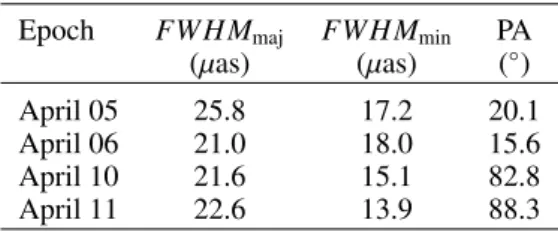
Table 1.CLEAN beam sizes of the EHT toward 3C 279.
Epoch FWHMmaj FWHMmin PA
(µas) (µas) (◦)
April 05 25.8 17.2 20.1
April 06 21.0 18.0 15.6
April 10 21.6 15.1 82.8
April 11 22.6 13.9 88.3
Notes. The beam sizes were obtained using Difmap and uniform weighting. We adopt a 20 µas circular Gaussian beam for all 3C 279 CLEAN images.
2.2. Imaging and model-fitting analysis
For imaging, we used frequency-averaged visibility data from the EHT-HOPS pipeline (see Paper III andBlackburn et al. 2019). We note that image reconstruction with 1.3 mm wavelength EHT data is particularly challenging because of the sparse (u, v) coverage, total loss of absolute atmospheric phase, and large gain fluctuations at some stations. In addition, the 2017 EHT observations lack relatively short baselines at .1 Gλ to robustly recover extended emission structure on VLBI scale at &100 µas (Paper IV). To ensure that the features we identi-fied in our reconstructed images are robust, the source images were generated by both traditional CLEAN and newer regular-ized maximum likelihood algorithms implemented in the fol-lowing programs: Difmap (Shepherd et al. 1994), eht-imaging (Chael et al. 2016,2018), and SMILI (Akiyama et al. 2017a,b). We used imaging pipelines for these three programs (see Paper IV) to generate a total of 12 images of 3C 279 (i.e., one per epoch per imaging method) within a limited field of view of ∼100 µas due to lack of short EHT 2017 baselines (Paper IV). In all methods, emission from the further extended milliarcsecond-scale jet (Fig. 4), which lies beyond the compact EHT field of view, was represented by a single large-scale Gaussian (see Paper IV for details). We then averaged the three pipeline images to obtain a representative image of the source at each epoch. We refer to Paper IV for the details of the imaging pipelines and image averaging procedures. In order to illustrate the EHT angu-lar resolution toward 3C 279, we show in Table1 the CLEAN beam sizes of the EHT 3C 279 data calculated by Difmap.
In order to parameterize bright and compact features in the source, we also performed Gaussian model-fitting analyses in two distinct ways. The first is the traditional VLBI model-fitting procedure (DIFMAP modelfit, which employs the Levenberg-Marquardt algorithm for non-linear fits) to reconstruct a static model with more than six components on each observation day. Related components were then identified and the evolution in their relative positions measured.
The second method utilizes T
hemis
, an EHT-specificanal-ysis package, using a parallel-tempered, affine invariant Markov chain Monte Carlo sampler (Broderick et al., in prep., and refer-ences therein). In this case, a fully time-variable, ten-component (nine compact and one large-scale) Gaussian component model was reconstructed to naturally facilitate the identification of fea-tures in subsequent observations and directly reconstruct their evolution. From this time variable model, component parameters and uncertainties are reconstructed for individual days. Addi-tional descriptions of the underlying model and T
hemis
anal-ysis can be found in AppendixA(also see Paper VI for more general details for the EHT model-fitting and model-comparison analysis).
In order to examine the reliability of the converged images and models, we also compared antenna gains reconstructed by amplitude self-calibration with both imaging and model-fitting software. Figure B.1 shows plots of antenna gain corrections for all days across different imaging pipelines and T
hemis
forLMT, which has the largest systematic gain uncertainties in the EHT 2017 observation (Papers III–VI). Consistent gain cor-rections across independent imaging methods and model-fitting analysis suggest that the results are robust against possible biases in each algorithm.
3. Results
3.1. First 230 GHz images
Figure3shows an overview of the 3C 279 jet structure in April 2017 at 43, 86, and 230 GHz, where the 43 and 86 GHz images are from quasi-simultaneous observations by the
VLBA-BU-BLAZAR 43 GHz (Jorstad et al. 2017) and the GMVA blazar
monitoring programs3, shown here for an illustration of the larger-scale jet structure. In Fig.4we show the final EHT 1.3 mm images of 3C 279 on April 5, 6, 10, and 11 obtained as described in Sect.2.2. The individual source images for all pipelines and epochs are shown in Fig.C.1. The images show two bright and somewhat extended emission regions, separated by ∼100 µas, with complex substructures within each of them. Hereafter we refer to the northern and southern complexes as C0 and C1, respectively. The C0 feature is substantially elongated in the NW-SE direction by ∼30−40 µas, as defined by the separation between its subcomponents (see Sect. 3.3). This elongation is perpendicular to the long-term larger-scale jet direction (SW; see, e.g., Jorstad et al. 2017). We find a prominent and rapid change of the brightness in the center of the C0 region over ∼6 days (see also Sect.3.3).
3.2. Inter-day closure phase variations
We show in Fig.5the closure phases of several long EHT tri-angles for all days. Remarkably, the ALMA-SMA-SMT trian-gle reveals large inter-day closure phase variations of ∼100◦ in
∼6 days. Comparable closure phase changes are also seen for other large triangles (Fig.5). We note that similar inter-day clo-sure phase changes were previously found in 3C 279 at 230 GHz byLu et al.(2013), but the much higher-sensitivity and longer-baseline data presented here reveal much more dramatic closure phase variations. This strongly implies the presence of inter-day variability of the surface brightness distribution and compact structure in the jet.
3.3. Model-fitting results
Values of parameters resulting from the Gaussian model-fitting analysis for all days, such as component flux densities, sizes, and relative positions are provided in Table D.1. Where these are obtained from T
hemis
, they are evaluated from thedynam-ical model at 6 UTC on each observation day. The component kinematics are displayed in Figs.6and7. Visibility amplitudes and closure phases of the self-calibrated data and the Gaussian model-fit are shown in Fig.D.1.
Quantitatively similar results were obtained on each day by
both Difmap modelfit and T
hemis
analyses; hereafter, we−3000 −2000 −1000 0 1000 Relative RA (μa ) −3000 −2000 −1000 0 1000 R el at iv e D ec ( μa ) 2017 April 16 / VLBA 43GHz −500 −250 0 250 Relative RA (μa ) −600 −400 −200 0 200 2017 April 01 / GMVA 86GHz −100 −50 0 50 Relative RA (μa ) −150 −100 −50 0 502017 April 11 / EHT 230GHz 10−2 10−1 100 10−2 10−1 100 0.0 0.2 0.4 0.6 0.8 1.0
Fig. 3.Illustration of multiwavelength 3C 279 jet structure in April 2017. The observing epochs, arrays, and frequencies are noted at the top of
each panel. The color bars show the pixel values in Jy beam−1. The white circles in the bottom left corners indicate the convolving beams. The
white rectangles shows the field of view of the next panels at the higher 86 and 230 GHz frequencies. We note that the centers of the images (0,0) correspond to the location of the peak of total intensity. (From left to right) the beam sizes are 150 × 380, 50 × 139, and 20 × 20 µas2. For a spatially
resolved emitting region, an intensity of 1 Jy beam−1 in the 43, 86, and 230 GHz images correspond to brightness temperatures of 1.16 × 10¹⁰,
2.37 × 10¹⁰, and 5.78 × 10¹⁰K, respectively. 90 as
April 05
E N 90 asApril 06
90 asApril 10
90 asApril 11
C0-0 C0-1 C0-2 C1-0 C1-1 C1-20.0
0.2
0.4
0.6
0.8
1.0
1.2
1.4
1.6
Intensity (Jy/Beam)
Fig. 4.EHT images of 3C 279 on each day, generated by three different pipelines, then aligned and averaged. See Paper IV for details on the
method. The circular 20 µas restoring beam is shown in the bottom right corner of each panel. The pixel values are in units of Jy beam−1. In each
panel, the contour levels are 5%, 12%, 25%, 50%, and 75% of the peak value. The component identification is shown in the April 11 panel and is only for illustration (see Fig.6).
focus on the T
hemis
results that naturally identify componentsacross observation epochs. We find that the closure phases, clo-sure amplitudes, and visibilities can be consistently described by a model consisting of the ten Gaussian components, with a reduced χ2of ∼1.3 for the best-fit models with ∼1.5% systematic
errors in the visibility amplitudes (and equivalently ∼2◦errors in
phases; see Paper III).
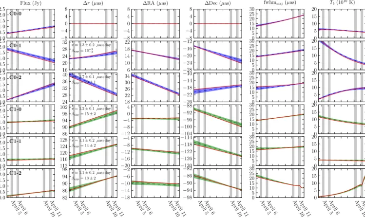
Six compact and bright features among the nine evolving components are the most robustly constrained across epochs. The other three extra components are much fainter (e.g., by an order of magnitude), and are located outside the intensity distri-butions reconstructed by imaging methods (Fig. 4). Therefore, we do not discuss these three components hereafter. Figure 8 summarizes the time evolution over all epochs of the parameters of these features. Three of them – C0-0, C0-1, and C0-2 – belong to the C0 region, while the remainder (labeled C1-0, C1-1, and C1-2) belong to the C1 region (see the rightmost panel of Figs. 4 and 6). We note that there are consistent, outward ∼1.1−1.2 µas day−1 proper motions of all C1 components when the C0-0 feature is used as a reference. In contrast, C0-1 moves perpendicular to its center position angle with respect to C0-0
with flux density decrease, and C0-2 moves toward C0-0 with a pronounced increase in its flux density (see Sect.3.4for more details).
Using the jet component parameters, we can compute their apparent brightness temperatures in the frame of the observer (thus not redshift or Doppler-boosting corrected), TB, as TB =
1.22 × 10¹²F/(ν2dmajdmin) K where for each component F is the
flux density in Jy, ν is the observing frequency in GHz, and dmaj,min are the major and minor full width at half maximum
(FWHM) sizes of the Gaussians in milliarcseconds, respectively. The TB values for all days are shown in Fig.8and Table D.1.
The apparent brightness temperatures are in the range of TB ∼ 1010−11K. We note that the C0-1 and C0-2 components show
particularly large flux and size variations, which essentially lead to rapid changes in the brightness temperature over the one-week observing period.
3.4. Kinematic reference
Because of the nontrivial, complicated motions of C0-1 and C0-2 with respect to C0-0, we also selected C0-1 and C0-2 as
19 20 21 22 GMST (h) 125 150 175 200 225 250 Closure Phase (deg)
ALMA-SMA-SMT
April 5 April 6 April 10 April 11 19 20 21 22 GMST (h) −100 −50 0 50 100 Closure Phase (deg)ALMA-LMT-SMA
17 18 19 20 21 22 GMST (h) −60 −40 −20 0 20 Closure Phase (deg)ALMA-LMT-SMT
Fig. 5. Example of the closure phase variation in 3C 279 over four
epochs for the large ALMA-SMT-SMA, ALMA-LMT-SMA, and ALMA-LMT-SMT triangles. The points show the data, and their error bars include 1.5% systematic visibility errors (Paper III). The solid lines show the model closure phases corresponding to the images from each pipeline and day, and the dashed lines represent the model closure phases of the average images shown in Fig.4. Regions constrained by predictions of the three independent image models are shaded.
alternative kinematic references and recalculated motions in order to see if the complex kinematics could be described more simply (e.g., simple radial outward motion in all com-ponents). We find that the component speeds are still compa-rable with the alternative references (although the directions of the proper motions are even more complicated), for example the
−25
0
25
Relative RA (μas)
−140
−120
−100
−80
−60
−40
−20
0
20
R
el
at
iv
e
De
c
(μ
as)
C0-0 C0-1 C0-2 C1-0 C1-1 C1-2 −10 0 10 20 30 40 Relative RA (μas) −30 −20 −10 0 10 R el at iv e De c (μ as)C0-0
C0-1
C0-2
−20 0Relative RA (μas)
−130 −120 −110 −100 −90 −80R
el
at
iv
e
De
c
(μ
as)
C1-0
C1-1
C1-2
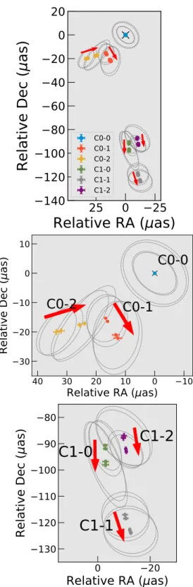
Fig. 6.Model-fit component kinematics during April 5–11. Top panel:
kinematics for all components. The center positions of different Gaus-sian components, and their uncertainties are color-coded (see legend). The Gaussian FWHM sizes are shown by dashed gray ellipses. The black cross at (0,0) indicates the kinematic reference (C0-0). Red arrows show the component motions; their lengths are proportional to the apparent velocities. Middle and bottom panel: same as the top panel, but zoomed in to the nuclear (C0) and extended jet regions (C1), respec-tively. We note that the center (0,0) in all panels is chosen as the center of C0-0, not the peak of total intensity.
C0 subcomponents moving toward the north (i.e., in the oppo-site direction to the large-scale jet; see Figs.7, top panel, and3)
−50
0
Relative RA (μas)
−125
−100
−75
−50
−25
0
25
R
el
at
iv
e
De
c
(μ
as)
C0-0 C0-1 C0-2 C1-0 C1-1 C1-2−50
0
Relative RA (μas)
−125
−100
−75
−50
−25
0
25
R
el
at
iv
e
De
c
(μ
as)
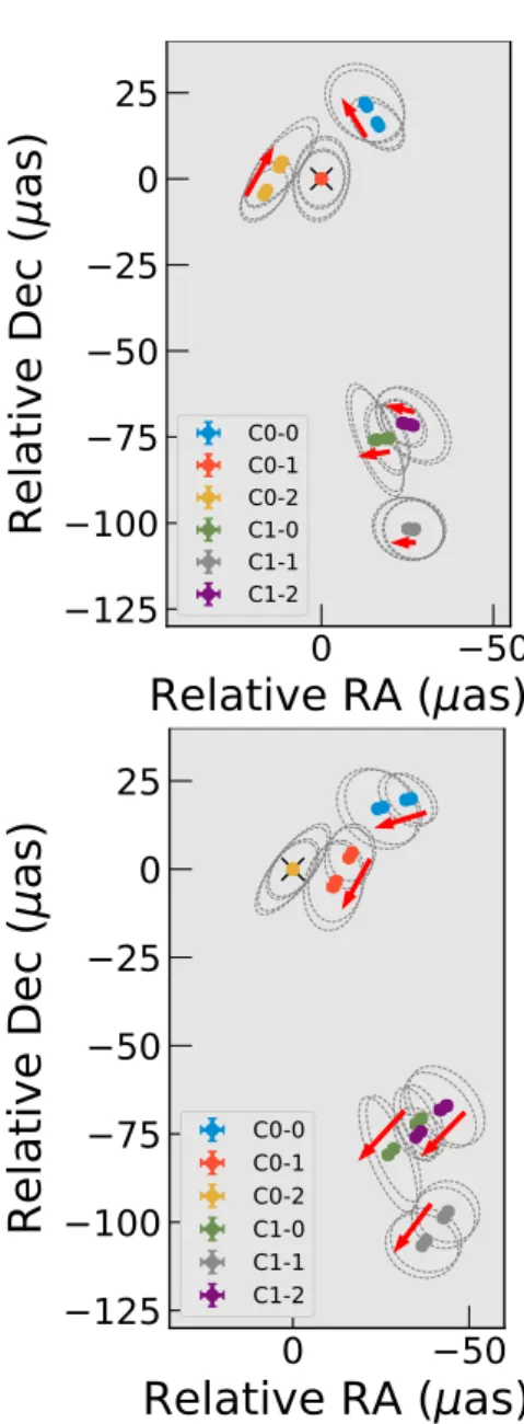
C0-0 C0-1 C0-2 C1-0 C1-1 C1-2Fig. 7.Same as Fig.6, but using C0-1 (top) and C0-2 (bottom) as
kine-matic references. We note the more complicated motions of other jet features in both panels compared to Fig.6.
and the C1 subcomponents moving toward the east (Fig.7, bot-tom panel) if C0-1 is chosen as the reference. Similar com-plex motions are seen when C0-2 is chosen as the reference. Therefore, choosing C0-0 as the kinematic reference provides a smoother transition of the kinematics from the inner EHT scale to the outer large jet (see Fig.3), and also helps avoid unneces-sary complexity in the interpretation given the limited available data, although this choice alone does not allow us to determine which of the three C0 subcomponents remains more station-ary in time (see Sect.4.3for more discussions from a physical perspective).
We also note that adopting C0-0 as the kinematic reference helps avoid false identification of the other C0 subcomponents, such as counterjet features. The expected jet-to-counterjet ratio of discrete emission features in 3C 279 can be computed as ((1+ β cos θ)/(1 − β cos θ))m−α, where β is the jet speed in units
of c; m = 2 or 3 for a continuous jet or a single component, respectively (see, e.g.,Urry & Padovani 1995); and α is the opti-cally thin spectral index (i.e., flux density S ∝ ν+α). If we adopt
α = −0.7, θ = 2◦, m= 3, and β = β
app/(sin θ + βappcos θ), where
βapp & 10 based on the observations, the expected brightness ratio is &1010; however, the observed brightness ratios of the C0
subcomponents are within an order of magnitude (TableD.1). Therefore, we should expect to find no counterjet features situ-ated to the north of the VLBI “core” (see Fig.7), although emit-ting features moving in a helically bent jet could perhaps produce this apparent backward motion if the jet is closely aligned to the line of sight (see Sect.4for a discussion).
In addition, we further note that the VLBI core is usu-ally defined as the most compact and brightest jet feature in the obtained images, and thus has the highest brightness tem-perature. It is interesting to note in Fig. 8 that the brightest component is not C0-0, but either C0-1 or C0-2, depending on the observing epochs. With this criterion, C0-1 and C0-2 might be still classified as the VLBI core. However, long-term and high-resolution observations of blazar jets find that com-pact and bright jet components near the VLBI core often have higher brightness temperatures than the cores determined by the jet kinematics (see, e.g.,Lisakov et al. 2017;Bruni et al. 2017; Jorstad et al. 2017). Thus, identifying C0-1 and C0-2 as the potential VLBI core based on the flux density and brightness temperature may not be strongly supported in our observations. Therefore, we adopt C0-0 as the VLBI core of 3C 279 in the following analysis.
4. Discussion
4.1. Elongated nuclear structure
The nuclear (C0 region) structure of 3C 279 resolved at the high-est 20 µas angular resolution is elongated perpendicular to the large-scale jet. This structure is seen in both independent imag-ing and model-fittimag-ing methods, and can be modeled as three bright features separated by ∼30−40 µas. This corresponds to a projected spatial scale of ∼2500−3400 Rsfor MBH= 8×10⁸M .
This morphology has not been commonly seen for 3C 279 by VLBA at 15 and 43 GHz (Jorstad et al. 2017; Lister et al. 2018). If the jet emission represents distribution of underlying synchrotron-emitting plasma, this peculiar structure can be inter-preted in various ways. Below we provide four possible interpre-tations.
Standard jet formation scenarios suggest relativistic jet launching by either angular momentum extraction from the spin-ning SMBH (Blandford & Znajek 1977) or magneto-centrifugal acceleration by an accretion disk (Blandford & Payne 1982), or by both mechanisms at the same time. In this context, a spatially resolved jet base, similar to the jet base morphology found in several nearby radio galaxies, in particular with limb-brightened jets (e.g., 3C 84; Giovannini et al. 2018, Cygnus A; Boccardi et al. 2016) is also possible. However these are viewed at a much larger angle to the line of sight than for 3C 279 and could provide an edge-on view of the limb-brightened jet base or the disk (thus thin elongated geometry if the accretion flow is not a sphere but has a finite height-to-radius ratio of, e.g., H/R . 1; see, e.g.,Yuan & Narayan 2014). However, for 3C 279 a nearly face-on view (θ ∼ 2◦) and thus a more rounded, thick emission
geometry is expected on the sky for the base of a circular jet or the accretion flow, in contrast to the observed images which show a narrow width along the global direction of the jet4.
4 This holds true, unless the plasma in the jet base moves at highly
relativistic speeds. In this case we could effectively observe the jet sys-tem in an edge-on view because most of observed radiation would have been emitted perpendicular to the jet in the jet co-moving frame, due to strong relativistic aberration.
0.0 0.5 1.0 1.5 2.0 2.5 Flux (Jy) C0-0 −8 −4 0 4 8 ∆r (µas) −8 −4 0 4 8 ∆RA (µas) −8 −4 0 4 8 ∆Dec (µas) 0 5 10 15 20 25 30 fwhmmaj(µas) 0 5 10 15 20 Tb(1010K) 0.0 0.5 1.0 1.5 2.0 2.5 C0-1 16 20 24 28 32 v = 1.3 ± 0.2 µas/day βapp= 16+3−2 6 10 14 18 22 −28 −24 −20 −16 −12 0 5 10 15 20 25 30 0 5 10 15 20 0.0 0.5 1.0 1.5 2.0 2.5 C0-2 24 28 32 36 40 v = 1.7± 0.1 µas/day βapp= 20± 1 18 22 26 30 34 −26 −22 −18 −14 −10 0 5 10 15 20 25 30 0 5 10 15 20 0.0 0.5 1.0 1.5 2.0 2.5 C1-0 86 90 94 98 102 v = 1.2± 0.1 µas/day βapp= 15± 2 −12 −8 −4 0 4 −104 −100 −96 −92 −88 0 5 10 15 20 25 30 0 5 10 15 20 0.0 0.5 1.0 1.5 2.0 2.5 C1-1 112 116 120 124 128 v = 1.1± 0.2 µas/day βapp= 14± 2 −20 −16 −12 −8 −4 −130 −126 −122 −118 −114 0 5 10 15 20 25 30 0 5 10 15 20 April 5 April 6 April 10 April 11 0.0 0.5 1.0 1.5 2.0 2.5 C1-2 April 5 April 6 April 10 April 11 82 86 90 94 98 v = 1.1 ± 0.2 µas/day βapp= 13± 2 April 5 April 6 April 10 April 11 −18 −14 −10 −6 −2 April 5 April 6 April 10 April 11 −98 −94 −90 −86 −82 April 5 April 6 April 10 April 11 0 5 10 15 20 25 30 April 5 April 6 April 10 April 11 0 5 10 15 20
Fig. 8.Model-fit parameters and their time evolution obtained by the T
hemis
time-evolving model-fitting (Sect.2.2). Each row shows a singlecomponent. Shaded regions indicate 95% confidence level at each time, the dashed line shows the median value, and the red solid lines indicate the best fit value. Observing epochs are shown by gray vertical bands. The component IDs are shown at the top left corner of the leftmost column. From left: flux density, radial distance with respect to C0-0, RA and Dec offsets with respect to C0-0, core mean FWHM sizes, and apparent brightness temperature.
Alternatively, the large transverse (to the downstream jet) size of the C0 region could correspond to a linear structure such as a site of large-scale magnetic reconnection, which could provide a long linear string of “plasmoids” (see, e.g., Blandford et al. 2017), or some oblique structure, like a shock or an oblique jet filament (e.g.,Marscher & Gear 1985;Hardee 2000). The former explanation would require continuous mag-netic reconnections along the jet during the observations. Per-haps the simplest and easiest way for this to happen is if the magnetic field in the jet were in the form of loops that become stretched out by cross-jet velocity gradients. Qualitatively, this would provide elongated loops where oppositely directed field lines are adjacent to each other and could reconnect in various locations. In this case, the predicted polarization electric vector position angle would be perpendicular to the elongated emission structure, which can be tested in the future by EHT linear polar-ization imaging.
It is also important to mention that the above scenarios do not exclude the possibility that the moving emission features are not necessarily associated with motions of the underlying plasma. This implies that the observed emission could only be patterns on the surface of the jet, such as propagating shocks or instabilities (e.g.,Lobanov & Zensus 2001). In this case, the observed bright components might represent only a small fraction of the entire broad jet.
For AGN jets such as 3C 279 seen at small viewing angles, however, it should be noted that a propagating component exe-cuting a slight bend in three dimensions can cross the line of sight and change the apparent inner jet position angle by
a substantial amount. The observed proper motions in the C0 region suggest that non-ballistic (i.e., curved) trajectories are required for C0-1 and C0-2 if they originated from C0-0. That is, the perpendicular motion of C0-1 compared to its position angle with respect to C0-0 could correspond to ∼90◦ apparent
jet bending. It is also worth noting that the contracting compo-nent motions within the C0 region are still present even if C0-1 or C0-2 are used as kinematic reference, which could imply a complex three-dimensional structure of the emitting jet plasma in the C0 region. Therefore, we investigate in Sect.4.2the kine-matics of the inner 3C 279 jet in more detail and constrain the potential three-dimensional jet geometry.
4.2. Jet kinematics on daily andµas scales
As briefly introduced in Sect.1, the kinematics of the 3C 279 jet revealed by previous interferometric imaging observations is complicated. Previous studies based on VLBA 15 and 43 GHz observations revealed a wide range of observed apparent speeds and jet bulk Lorentz factors at various locations and epochs (e.g., βappranging from a few to ∼20 c andΓ ∼ 10−40)5, and changing directions of jet proper motions, which is often accompanied by apparent increase of βapp(see references in Sect.1). There is
evi-dence obtained from studies of large samples (e.g.,Homan et al. 2015) that intrinsic jet acceleration (i.e., increasingΓ) is required to explain these phenomena. However,Homan et al.(2003) and
5 Doppler factor δ = (Γ(1 − β cos θ))−1, with the bulk Lorentz factor
Jorstad et al.(2004) show specifically for 3C 279 that the chang-ing motion vectors and increaschang-ing βapp can be nicely explained
simply by varying the viewing angle along the outflow, without necessarily changing the intrinsic bulk Lorentz factor. In the light of this, we investigate the kinematics of the C0 and C1 regions, focusing on a similar geometrical model (i.e., bent jet) and using the observed component properties. In the following we assume that the dynamical center of the jet system is C0-0 (see Sect.3.3). 4.2.1. C0 region
Before describing details, we note that the pure jet bending scenario is physically well motivated because (1) the kinemat-ics of C0 subcomponents clearly exclude simple radial outward motions, (2) the separation between C0-1 and C0-2 is small (∼12−17 µas ∼0.08−0.11 pc projected) and perhaps too short for a significant jet acceleration or deceleration to occur, and (3) the jet bending model requires less fine-tuning than more compli-cated scenarios in which, for example, a jet changes both the bulk Lorentz factor and viewing angle. Accordingly, we assume that both C0-1 and C0-2 have the same bulk Lorentz factors but different viewing angles.
Using the special relativity relationships (Footnote 5), we show in Fig. 9 possible combinations of viewing angles and Doppler factors for various values of Lorentz factors in the plane of βapp and δ. By inspecting the plot it is clear thatΓ = 20 is
needed to explain βappof both C0-1 and C0-2 using a constant
Γ. If we take Γ = 20 as a nominal value, it can be seen that a viewing angle of θ ∼ 2.9◦ is required for C0-2, while θ can
be ∼1.5◦ or ∼5.5◦ for C0-1. We can then examine whether the
viewing angle should be smaller or larger for C0-1 by assuming that the intrinsic flux densities of C0-1 and C0-2 are identical but observed differently only due to Doppler boosting, and then by computing ratios of the Doppler factors for these components.
The flux densities of C0-1, SC0−1, and C0-2, SC0−2result in
a flux density ratio of SC0−1/SC0−2∼0.6−5.9 (TableD.1). Since
the observed flux density ratio is proportional to δm−α, where
m = 2 or 3 as defined in Sect.3.4, the required Doppler factor ratio should be δC0−1/δC0−2 = (SC0−1/SC0−2)1/(m−α). Assuming
m = 3 and α = −0.7, we obtain δC0−1/δC0−2 ∼ 0.87−1.62. As
shown in Fig.9, θ= 2.9◦could explain C0-2 withΓ = 20, and
the corresponding Doppler factor is δC0−2 ∼ 20. Similarly for
C0-1 andΓ = 20, θ = 1.5◦and 5.5◦result in Doppler factors of
δC0−1 ∼ 32 and ∼8, respectively. The Doppler factor ratios are then δC0−1/δC0−2 ∼ 1.6 or ∼0.4 for the larger and smaller
val-ues of θ for C0-2, respectively. Both ratios broadly agree with what is required to explain the observed flux density ratio, con-sidering potentially large uncertainties in those numbers due to our assumptions. Therefore, we could conclude that both view-ing angles for C0-2 are consistent with observations, although the rapid time variability of C0-1 may prefer the larger Doppler factor and accordingly smaller viewing angle (Fig.8). It should be noted, however, that these calculations do not exclude higher Lorentz factors for both components, and therefore we constrain Γ ≥ 20 for both C0-1 and C0-2. Table2summarizes the possible values of θ,Γ, and δ for C0-1 and C0-2, as estimated based on the above assumptions.
Importantly, we note that the viewing angles of C0-1 and C0-2 can differ from each other by a few degrees. This amount is similar to the large 3C 279 jet inclination, θ ∼ 2◦, which is
estimated from long-term VLBA 43 GHz monitoring of the jet kinematics (Jorstad et al. 2017). It appears that these small view-ing angle differences could be sufficient to explain the almost 90◦ position angle offsets of C0-1 and C0-2 relative to the
10.0 12.5 15.0 17.5 20.0 22.5 25.0
Apparent speed (
app)
10
12
3
4
5
6
78
9
20
30
40
50
60
70
80
Do
pp
ler
fa
cto
r (
)
= 0.5 = 1.5 = 2.9 = 4.5 = 5.7 = 7.0 = 13 = 16 = 20 = 25 = 30 C0-1: = 32 C0-1: = 8 C0-2: = 20Fig. 9.Plane of apparent speed (βapp) and Doppler factor (δ). Solid and
dashed lines correspond to constant values of bulk Lorenz factors and viewing angles, respectively. The blue and green triangles and red cir-cle show possible values of βappand δ assuming the sameΓ = 20 for
C0-1 and C0-2, respectively. The vertical black lines correspond to the βappvalues of C0-1 and C0-2. The red and blue shaded areas indicate
uncertainties of βappfor C0-1 and C0-2, respectively.
Table 2.Summary of geometric and dynamical properties of the jet components discussed in Sects.4.2.1and4.2.2.
ID βapp θ Γ δ
(c) (◦)
Curved jet case(a)
C0-1 16+3
−2 ≤1.5 ≥20 ≥32
C0-2 20 ± 1 ≤2.9 ≥20 ≥20
C1-0/1/2 (13−15) ± 2 ≥6−8 ≥20 ≤5−7
Straight jet case(b)
C1-0/1/2 (13−15) ± 2 2 16−17 24−25
Notes.(a)The same Lorentz factor but different viewing angles for the jet features. For C0 subcomponents we presume the small θ case, while for C1 we presume the large θ case (see Sects.4.2.1and4.2.2).(b)Assumes
a constant fixed viewing angle of θ= 2◦.
SW-oriented large-scale jet. This means that a deprojection of ∼90◦ angle difference on the sky to a θ = 2◦jet system would
correspond to a jet viewing angle change of ∼90◦sin(1◦−2◦) ∼
1.6◦−3.1◦. This small amount of θ offset is not in contradiction
with the estimations of the jet viewing angle differences for C0-1 and C0-2, as shown above.
4.2.2. C1 region
In contrast to the C0 region, the three subcomponents in C1 have comparable apparent speeds (βapp ∼ 13−15), and their
posi-tion angles with respect to C0-0 are all in a narrow range of ∼ −(173◦−178◦), which are aligned to the directions of their
motion vectors (PA ∼ −(160◦−180◦)). Therefore, we can
reason-ably presume that these components share common kinematic and geometric properties.
We could extend the analysis in Sect.4.2.1to the C1 region, that is assuming a constant Γ = 20 for all the components to estimate their different viewing angles. We show in Fig.10the same βapp and δ plane but for the C1 subcomponents, which is
5.0 7.5 10.0 12.5 15.0 17.5 20.0 22.5 25.0
Apparent speed (
app)
10
12
3
4
5
6
78
9
20
30
40
50
60
70
Do
pp
ler
fa
cto
r (
)
= 0.5 = 1.2 = 2.9 = 4.5 = 6.3 = 7.7 = 11 = 16 = 20 = 25 C0-1: = 32 C0-1: = 8 C0-2: = 20Fig. 10.Same as Fig.9, but for C1. The vertical solid black lines
cor-respond to βapp values of the C1 subcomponents and the gray shaded
area shows their uncertainties. For comparison, the model values for C0 components withΓ = 20 are also shown using the same symbols as in Fig.9. The ranges of the axes are different from Fig.9.
used to constrain reasonable ranges of θ and the corresponding δ. For βapp = 13−15, there are two possible sets of parameters,
which are (i) θ ∼ 6◦−8◦and δ ∼ 5−7, and (ii) θ ∼ 1.0◦−1.5◦and
δ ∼ 33−35. We note that there is a similar ambiguity in determin-ing whether the jet bends closer to or away from the line of sight. Nevertheless, we could consider that weaker time variability of the C1-0 and C1-1 components might prefer smaller Doppler factor values (i.e., larger θ), while C1-2 shows stronger variabil-ity and thus could have larger Doppler boosting (i.e., smaller θ). Alternatively, dynamical properties of C1 could be better estimated by simply adopting the viewing angle of the larger-scale jet (θ ∼ 2◦; Jorstad et al. 2017) because the motions of
the C1 subcomponents are nearly parallel to the jet downstream (Fig.3). Using θ= 2◦, we obtainΓ ∼ 16−17 and δ ∼ 24−25.
Taken all together, the ranges of Lorentz factors for C1 are comparable to those found from the 3C 279 jet on larger scales and at longer wavelengths (&103pc or &105R
s
pro-jected;Bloom et al. 2013;Lister et al. 2016;Jorstad et al. 2017; Rani et al. 2018), and also those estimated from radio total flux variability (e.g.,Hovatta et al. 2009). The values of θ,Γ, and δ for C1 are also summarized in Table2.
4.3. Physical implications
In conclusion, it appears that the peculiar C0 structure could be described by a jet closely aligned to the line of sight, but bent by small angles, and the projection of the overall bent geom-etry to the sky. In this perspective, it is also worth noting that in a previous 230 GHz VLBI experiment on 2011 March 29– April 4, a similar nuclear morphology was found in 3C 279 based on a model-fitting approach (Lu et al. 2013). After 2011 December, this structure became resolved by the VLBA at 43 GHz as a bright moving feature situated at a position angle of initially ∼150◦, and later at ∼−170◦ relative to the 43 GHz
core (Aleksi´c et al. 2014; Jorstad et al. 2017), confirming the jet bending scenario (the VLBA 7 mm kinematics is shown in Fig.E.1). Notably, the overall situation of the source in 2011 is similar to the jet geometry we discussed in Sect.4.2.1. This sug-gests that the inner jet bending may commonly occur in 3C 279. In this respect it is interesting to note that a similar extremely
bent jet morphology is sometimes observed in several AGN on small angular scales, especially when the object is in a flar-ing state at multiple wavelengths (e.g., 1156+295 –Hong et al. 2004;Zhao et al. 2011; PKS 2136+141 –Savolainen et al. 2006;
OJ 287 – Agudo et al. 2012; Hodgson et al. 2017; 3C 345
– Lobanov & Roland 2005; CTA 102 – Fromm et al. 2013; Casadio et al. 2015; 0836+710 –Perucho et al. 2012). The flare is often interpreted as the result of an increase in Doppler beam-ing of the emission due to the jet bendbeam-ing closer to the line of sight.
There are several possible explanations for the physical origin of the jet bending. First, precession of a jet noz-zle, which is induced by propagation of perturbations orig-inating from the accretion disk and BH due to the Lense-Thirring effect (Bardeen & Petterson 1975) or even binary black holes, may display somewhat periodic jet wobbling over time. Abraham & Carrara(1998) and more recentlyQian et al.(2019) suggest such a physical model for 3C 279 with a precession period of ∼22 yr. However, we note that the similar erratic inner jet position angle in 2011 and 2017 seen by the EHT implies a precession period of .6 yr if the jet wobbling is periodic. The mismatching periods would exclude this possibility. Second, it should be noted that the C0-1 component is moving toward C1 and the jet downstream (Fig.3), and thus the component is being aligned to the larger scale jet during the observing period. The above-mentioned time evolution of the 3C 279 jet structure dur-ing 2011 also suggests that the initially bent jet component in the source later aligned with the downstream emission. The jet alignment in a single preferred direction could indicate that the outflow is being actively collimated to a pre-established chan-nel on these small spatial scales, as similarly observed in other sources as well (see discussions inHoman et al. 2015). Third, an internally rotating jet, in which emission regions are located along strong toroidal magnetic field lines, can also reproduce gradual jet bending features in the images (e.g., Molina et al. 2014). Such a scenario is supported by theoretical studies of jet launching and propagation (see, e.g., Tchekhovskoy 2015and references therein), and also observations of inner jet dynam-ics in nearby radio galaxies (e.g., Mertens et al. 2016) and smooth variation of linear polarization of many AGN jets in time and space (e.g., Asada et al. 2002; Marscher et al. 2008; Hovatta et al. 2012; Kiehlmann et al. 2016). Whether one of these scenarios is more favored than others is difficult to deter-mine, however. Joint constraints on the model parameters with additional data, for instance with linear polarization time vari-ability information (Nalewajko 2010), should prove fruitful.
We also note that the apparent jet speed and Lorentz fac-tor of C1 are comparable to those in the outer jet (Sect.4.2.2). This suggests that intrinsic acceleration of the jet (i.e.,
increas-ing Γ) would occur upstream of C1. This puts upper limits
on the spatial extension of the intrinsic jet acceleration zone of 3C 279 to be within .100 µas from the core, C0-0, which is 0.65 pc ∼8500 Rs projected distances (∼19 pc ∼2.4 × 10⁶Rs
deprojected with θ = 2◦). If the observed motions of
C0-1 and C0-2 can be described by similar bulk Lorentz fac-tors as C1, the intrinsic acceleration zone should be located at much more upstream of the jet, that is within .30−40 µas core separation ∼0.20−0.26 pc ∼2600−3400 Rs projected
dis-tances (∼6−7 pc ∼(7.3−9.7) × 104R
sdeprojected).
4.4. Low brightness temperature at 230 GHz
The innermost jet brightness temperature provides us with insight about the jet plasma acceleration and radiative evolution
further downstream (e.g., Readhead 1994; Marscher 1995; Schinzel et al. 2012;Fromm et al. 2013). The observed bright-ness temperatures of the subnuclear components within C0 are in the range of TB ∼ 1010−1011K (Fig.8). We note that these
measurements are made in the observer’s frame, while the intrin-sic brightness temperature of the plasma in the fluid frame, T0
B,
is lowered by the Doppler factor δ, that is T0
B= TB(1+z)/δ.
Con-sidering Doppler factors of δ ∼ 20 or even larger values due to possibly curved jet geometry (Sect.4.2), an order of magnitude lower intrinsic brightness temperature of T0
B ∼ 109−1010K is
possible. This is a significantly lower value compared to the long millimeter or centermeter wavelength VLBI core T0
B(e.g., TB>
1012K and T0
B ∼ 1011−12K; Kovalev et al. 2005; Jorstad et al.
2017) and also the inverse Compton limit, T0
B ∼ 5 × 10¹¹K
(Kellermann & Pauliny-Toth 1969).
It is challenging to make a straightforward interpretation of the low brightness temperature without knowing the level of syn-chrotron opacity at 230 GHz on 20 µas scales. Nevertheless, we provide two possible implications below.
First, it is worth noting that a trend of decreasing brightness temperature with increasing observing frequencies was previ-ously seen in a number of AGN jet cores in the frequency range of 2−86 GHz (e.g.,Lee et al. 2016;Nair et al. 2019). This trend is often interpreted as an indication of acceleration of underlying jet outflow, based on the following considerations. In the stan-dard model of relativistic jet (Blandford & Königl 1979), the sta-tionary radio VLBI core structure corresponds to a region with high synchrotron opacity (τ ∼ 1) at the corresponding observing frequency. In multiwavelength VLBI observations, the opacity effect appears as a shift in the apparent core position at different frequencies (i.e., the core located more upstream of the outflow at higher frequencies), which is commonly referred to as a “core-shift” (e.g.,Lobanov 1998). In this picture, higher frequency TB
measurements reveal physical conditions of the jet closer to its origin, if the core TB represents surface brightness of
underly-ing plasma outflow. In addition, we could further assume that the intrinsic brightness temperature of the plasma underlying the compact core is not frequency-dependent and remains the same over short distances (i.e., the coreshift distances). It then fol-lows that higher TBat lower frequencies could only be explained
by higher outflow speed further downstream, and consequent Doppler boosting of the emission to increase the observed TB.
It is tempting to apply this framework to the EHT 230 GHz brightness temperature measurement of 3C 279. The consis-tent apparent jet speeds of ∼10−20 c seen near the EHT core and further downstream in the jet at centimeter wave-lengths, however, does not strongly support the jet accelera-tion scenario. Instead, the brightness temperature can simply decrease with increasing frequency if the observing frequency is higher than the synchrotron self-absorption turn-over frequency (Rybicki & Lightman 1979). The low brightness temperature at 230 GHz can therefore be alternatively understood as a signature of low opacity in the core region at 1.3 mm. The ALMA phased-array data of 3C 279 from our observations show a steep spectral index of α= −(0.6 ± 0.06) at 230 GHz (seeGoddi et al. 2019), which supports this conclusion, although the ALMA measure-ments do not spatially resolve the microarcsecond-scale jet.
If, however, the compact VLBI core region still remains opti-cally thick up to 230 GHz, the observed low TB values could
be compared to the energy equipartition brightness temperatures (T0
B,eq ∼ 5 × 10¹⁰K; Readhead 1994), which is significantly
higher than T0
B derived from the EHT measurements. The
lower T0
B than the particle-to-magnetic field energy density
equipartition T0
B,eq would then suggest that the innermost jet of
3C 279 may be magnetically dominated, contrary to previous conclusions that the jet plasma has low magnetization in 3C 279 (see, e.g., discussions inHayashida et al. 2015;Ackermann et al. 2016). While high particle-to-magnetic energy density ratios are seen in other AGN especially during flaring activities (e.g., Jorstad et al. 2017;Algaba et al. 2018), low brightness temper-ature associated with potentially magnetically dominated jet is also seen in the nuclear region of other nearby AGN jets, such as M 87 (e.g., see discussions inKim et al. 2018). According to the standard model of jet launching and propagation, magnetic energy density is expected to be dominant in a jet up to central engine distances of ∼105R
s(seeBoccardi et al. 2017and
refer-ences therein). Considering the spatial scales of the EHT obser-vations of 3C 279 (20 µas∼ 1700 Rs), it is not impossible that the
observed innermost 3C 279 jet is indeed magnetic energy dom-inated. Nevertheless, future spectral decomposition and polari-metric analysis on the 20 µas scale with multifrequency EHT observations should determine the jet core opacity at 230 GHz, in order to provide an unambiguous interpretation of the remark-ably low T0
Bvalues.
4.5. Connection toγ-ray emission in 3C 279
During the EHT observations in April 2017, 3C 279 was in a highly active and variable state at γ-ray energies (see, e.g., Larionov et al. 2020). Here we briefly discuss possible implica-tions of the innermost 3C 279 jet kinematics revealed by the EHT observations on the γ-ray emission of the source. Generally, the jet speeds measured closest to the jet origin are important in order to understand the origin of γ-ray emission in blazars. One of most plausible scenarios explaining γ-ray emission in blazars is inverse Compton (IC) scattering of seed photons from within or around the relativistic jet, while details of the IC models vary depending on the assumptions of the background photon fields (see, e.g., Madejski & Sikora 2016). Observationally, bright γ-ray flares from blazars are often associated with emergence from the VLBI core of new, compact jet features, which travel toward the jet downstream (e.g.,Jorstad & Marscher 2016). This association implies that the IC process may occur near (or even upstream of) the VLBI core. Therefore, observational constraints on the innermost jet speed is crucial for an accurate modeling of the IC process.
The EHT measurements of the proper motion suggest a
minimum Lorentz factor of Γ & 20 at core separations
≤100 µas. On the other hand, much higher Lorentz factors of Γ & 100 are derived from the observations of rapid γ-ray flares (Ackermann et al. 2016). To accommodate the lower limit ofΓ from the EHT observations with the larger Lorentz factors from the jet kinematics and γ-ray variability, viewing angles smaller than θ < 1◦ in the region C0-1 and C0-2 may be considered.
For such small angles, Doppler factors of ∼100 could be reached, which are sufficient to explain the observed γ-ray variability. On the other hand, we note that the continued VLBA 43 GHz monitoring of the source during 2015−2018 now suggests faster motion and higher Lorentz-factors ofΓ & 37 than in the past (Larionov et al. 2020). As the authors note, the local values of Γ can be even larger (e.g., ∼70) if fast “mini-jets” are embed-ded within the main flow (e.g.,Giannios et al. 2009) or if mul-tiple, turbulent emitting zones are present (e.g.,Narayan & Piran 2012;Marscher 2014). The latter could increase the localΓ val-ues by factors of a few. Future detailed modeling of the broadband spectral energy distribution during the EHT 2017 campaign will