HAL Id: hal-01992793
https://hal.sorbonne-universite.fr/hal-01992793
Submitted on 24 Jan 2019HAL is a multi-disciplinary open access archive for the deposit and dissemination of sci-entific research documents, whether they are pub-lished or not. The documents may come from teaching and research institutions in France or abroad, or from public or private research centers.
L’archive ouverte pluridisciplinaire HAL, est destinée au dépôt et à la diffusion de documents scientifiques de niveau recherche, publiés ou non, émanant des établissements d’enseignement et de recherche français ou étrangers, des laboratoires publics ou privés.
Transit spectroscopy of temperate Jupiters with ARIEL:
a feasibility study
Thérèse Encrenaz, G. Tinetti, A. Coustenis
To cite this version:
Thérèse Encrenaz, G. Tinetti, A. Coustenis. Transit spectroscopy of temperate Jupiters with ARIEL: a feasibility study. Experimental Astronomy, Springer Link, 2018, 46 (1), pp.31-44. �10.1007/s10686-017-9561-2�. �hal-01992793�
Transit spectroscopy of temperate Jupiters with ARIEL:
A feasibility study
T. Encrenaz1, G. Tinetti2 and A. Coustenis1
1 LESIA, Paris Observatory, CNRS, PSL Universities, UPMC, UDD 2 Department of Physics and Astronomy, University College London
Submitted to Experimental Astronomy ARIEL Special Issue
Revised version September 2017
Corresponding author:
Thérèse Encrenaz
LESIA, Observatoire de Paris, CNRS, PSL Universities, UPMC, UDD Observatoire de Paris 5 place Janssen 92195 Meudon, France Tel: 33 1 45 07 76 91 Fax: 33 1 45 07 28 06 e-mail: [email protected]
Abstract
Several temperate Jupiters have been discovered to date, but most of them remain to be detected. In this note, we analyse the expected infrared transmission spectrum of a temperate Jupiter, with an equilibrium temperature ranging between 350 and 500 K. We estimate its expected amplitude signal through a primary transit, and we analyse the best conditions for the host star to be filled in order to optimize the S/N ratio of its transmission spectrum. Calculations show that temperate Jupiters around M stars could have an amplitude signal higher than 10-4 in primary transits, with revolution periods of
a few tens of days and transit durations of a few hours. In order to enlarge the sampling of exoplanets to be observed with ARIEL (presently focussed on objects warmer than 500 K), such objects could be considered as additional possible targets for the mission.
1. Introduction
Temperate Jupiters, with equilibrium temperatures ranging between 350 and 500 K, are not expected to exist according to the standard nucleation model, which requires that giant planets are formed at large distances from their host star, at temperatures low enough for water and other hydrogenated molecules to be in the form of ices (see e.g. Pollack et al. 1996). However, several temperate exoplanets with radii larger than half the Jupiter one and with periods ranging between 100 and 300 days have been detected around F, G and K stars (some examples are listed in Table 1, for semi-major axes ranging between 0.5 and 1.0 AU an eccentricities smaller than 0.1). It can be seen that their equilibrium temperatures range between 250 and 500 K. Their presence at relatively close distances to their host star might be the result of migration processes, or other possible formation mechanisms, still to be investigated. Although most of the objects detected so far are not suitable or probably too faint for transit spectroscopy, their detection demonstrates that this category of objects actually exists. If such objects are also transiting around low-mass stars, they would be suitable targets for transit spectroscopy, in particular with the ARIEL space mission. Future surveys with space missions like GAIA (Global Astrometric Interferometer for Astrophysics), but also CHEOPS (CHaracterizing ExOPlanets Satellite), TESS (Transiting Exoplanet Survey Satellite) or PLATO (PLAnetary Transits and Oscillations of stars), are likely to provide new targets for this category of exoplanets.
Table 1
Examples of temperate giant exoplanets detected around F, G and K stars, with a mass larger than 0.5 Jovian mass and an eccentricity smaller than 0.1 (from www.exoplanets.eu). The equilibrium temperature is calculated assuming an albedo a = 0.03 and a fast-rotating planet (Equation 4, see text below, Section 2).
Name MP(MJ) P(d) D(AU) e Spectral
type M* (Ms) T(K) P HD 134113 b 47 202 0.64 0.089 F9 V 0.81 295 HD 233604 b 6.6 192 0.747 0.05 K5 1.5 434 HD 28185 b 5.7 383 1.03 0.07 G5 1.24 320 HD 32518 b 3.04 157 0.59 0.01 K1 III 1.13 395 HD 159243 c 1.9 248 0.8 0.075 G0 V 1.125 338 HD 9446 c 1.82 193 0.654 0.06 G5 V 1.0 342 HD 141399 c 1.33 202 0.69 0.048 K0 V 1.07 390 HD 231701 b 1.08 142 0.53 0.096 F8 V 1.14 419 Kepler-11 g 0.95 118 0.46 0.0 G 0.95 392 HD 92788 c 0.9 162 0.6 0.04 G5 1.13 392 HD 37124 b 0.675 154 0.53 0.054 G4 V 0.83 331 HD 45364 c 0.66 343 0.897 0.097 K0 V 0.82 252 Mu Ara d 0.52 310 0.92 0.07 G3 IV-V 1.08 306
In this paper, we investigate what could be the infrared spectrum of a temperate Jupiter and we study its detectability with the ARIEL space mission using transit spectroscopy,
both through primary transit and secondary transit. We then analyse the most favorable type of star in order to optimize the primary transit signal.
The objective of ARIEL is the characterization of a large sample of exoplanets’atmospheres (500 – 1000 targets) using transit spectroscopy in the mid-infrared range (2 – 8 m), with a resolving power between 100 and 200. It consists in an off-axis 90-cm telescope, passively cooled at 60-70 K, with a spectrometer cooled at 50 K and MCT detectors also cooled at 40 K. The stellar light is simultaneously recorded by a photometer operating at 1 – 2 m. ARIEL is primarily designed for observing various kinds of exoplanets with equilibrium temperatures higher than 500 K. In order to enlarge the diversity of targets observable with ARIEL, we analyze in this paper the feasibility of observing cooler giant exoplanets, with equilibrium temperatures ranging between 350 and 500 K.
2. The equilibrium temperature of an exoplanet
The equilibrium temperature Te of a slow-rotating exoplanet is given by this equation:
Te = (1 – a)0.25 x 331.0 x (T*/5770) x R*0.5)/ D0.5 (1)
or
Te = (1 – a)0.25 x 331.0 x (M*)3/4)/ D0.5 (2)
where a is the albedo, T* the effective temperature of the star (in K), R* its radius and M* its mass (in solar units), and D the distance of the exoplanet to the star (in AU). For a fast-rotating exoplanet, these equations become:
Te = (1 – a)0.25 x 279.0 x (T*/5770) x R*0.5)/ D0.5 (3)
or
Te = (1 – a)0.25 x 279.0 x (M*)3/4)/ D0.5 (4)
In the case of a solar type star, taking as extreme conditions albedo values of 0.3 and 0.03 (as most commonly observed in the solar system), we find distances to the host star ranging between 0.26 AU (for a fast-rotating planet, Te = 500 K and a = 0.3) and 0.9 AU
(for a slow-rotating planet, Te = 350 K and a = 0.03). For a solar-type star, the
corresponding revolution periods range between 48 days and 312 days. The periods decrease if low-mass stars are considered. In order to perform transit spectroscopy of temperate Jupiters, several transits have to be performed over the lifetime of the mission, so, in what follows, we will focus on stars less massive than the Sun which allow a larger number of transits.
In order to estimate the equilibrium temperature of an exoplanet, we need to make an assumption on its rotation period. As a first approximation, this can be estimated from a comparison of its distance to the star versus the tidal lock radius, i.e. the distance to the star within which synchronous rotation takes place as a result of tidal forces. According
to Murray and Dermott (1999) and Léger et al. (2009), the characteristic time for a planet to reach synchronous rotation is given by:
synch = l(n –P)l x MP x D6 x I x Q/k2P /[3/2 xG x RP3 x M*2] (5)
where n is the mean motion of the revolution rate of the planet, is its rotation rate, I is its moment of inertia, Q its dissipation constant, k2P its Love number of second order. MP
is the planetary mass and RP is its radius, D is the distance of the planet to the star, M* is
the stellar mass and G is the gravitational constant. It can be seen that for a given planet,
synch is proportional to D6/M*2. Thus, the tidal lock radius Dsynch, corresponding to a
given value of synch, is proportional to [M*]1/3. This is shown in the study by Kasting et
al. (1993; Fig. 16) who indicate the tidal lock radius for Earth-like exoplanets; they find a tidal-lock radius Dsynch of 0.4 AU for a solar-mass star and 0.2 AU for a star of 0.1 solar
mass. The corresponding revolution period of the planet is about 90 days, independent of the stellar mass.
For the present study, we need to estimate the tidal lock radius for giant exoplanets. In the lack of information about the values of the tidal parameters of these planets, we can compare the physical and tidal parameters of giant solar system planets as compared with terrestrial ones. Planetary moments of inertia range between 0.2 and 0.35. Rotation periods of the Earth and Jupiter are within a factor of 2. The Q/k2P factor is about 1000
for the Earth while this quantity is in the range 103 – 105 for Jupiter and Saturn (Lainey,
2006). This leads to a synch value between 1 and 100 times the terrestrial value for giant exoplanets. Accordingly, Dsynch is expected to range between the terrestrial value (as
indicated by Kasting et al. 1993) and half this value, and the corresponding limit for the revolution period is between 90 days and 33 days. As a consequence, the values of Te
shown in Table 1 are calculated using Equation 4, corresponding to fast-rotating exoplanets.
3. The atmosphere of a temperate Jupiter
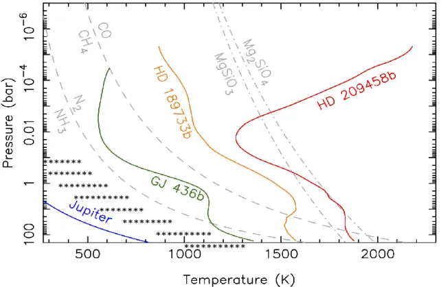
Let us assume a Jupiter-type planet with an equilibrium temperature ranging between 350 K and 500 K under thermochemical equilibrium. The atmosphere is expected to be characterized by a troposphere where the temperature decreases as the altitude increases, following the adiabatic gradient. The atmospheric composition is expected to be dominated by hydrogen and helium. As for solar system giant planets, we assume for the tropopause a pressure level of 0.1 bar, constrained by the hydrogen and helium opacities. Figure 1 shows a P(T) diagram of a temperate Jupiter. If we assume thermochemical equilibrium, it can be seen that, in the exoplanet’s environment, nitrogen and carbon are expected to be in the form of NH3 and CH4 respectively. In the
Figure 1. The T(P) diagram of a temperate Jupiter with an equilibrium temperature ranging between 350 K and 500 K. The range corresponding to temperate Jupiters is shown with the black dots. It can be seen that carbon and nitrogen are expected to be in the form of NH3 and CH4 respectively. The figure is adapted from the EChO proposal (Tinetti et al. 2011).
In the troposphere, according to thermochemical equilibrium, CH4, NH3 and H2O are
expected to be the main minor species. We assume for them, in the troposphere, the cosmic abundances. We know, however, that in the case of the giant planets of the solar system, these molecules are enriched by a factor about 4 as a result of the nucleation formation Owen and Encrenaz 2006). This factor of 4 depends upon the relative mass of the initial icy core with respect to the total mass of the planet (3% in the case of Jupiter); in the case of Saturn, for which the initial icy core is about 15% of the total mass, the expected enrichment is a factor of about 9. When the icy core becomes a major part of the total mass of the giant planet, as for Uranus and Neptune, the enrichment factor is above 30-40. We note that, in any case, in the nucleation model, the enrichments are expected to be the same for O, C, and N; so we can assume that the relative abundances of CH4, NH3 and H2O in the troposphere of the exoplanet are consistent with the cosmic
abundances (Grevesse et al. 2005). In our calculations, we assume for CH4 and NH3 the
same abundances as measured in Jupiter below the condensation levels: CH4/H2 = 2 x
10-3 (Encrenaz et al. 1999), NH3/H2 = 2 x 10⁻⁴ (Encrenaz et al. 1999, Bolton et al. 2017).
For H2O we assume H2O/H2 = 4 x 10⁻³ below the water cloud level. We thus adopt
H2O:CH4:NH3 = 2:1:0.1. It must be noted that these numbers are no more than examples,
chosen to build a typical spectrum of a temperate Jupiter.
With respect to the true atmosphere of Jupiter, the main difference of a temperate Jupiter is that there is no cold trap at the tropopause: at a temperature above 350 K, all molecules, including H2O and NH3, keep a constant mixing ratio with the altitude, up to a
level where they become photo-dissociated. As a result, the infrared spectrum of a temperate Jupiter is expected to be fully dominated by CH4, NH3 and H2O.
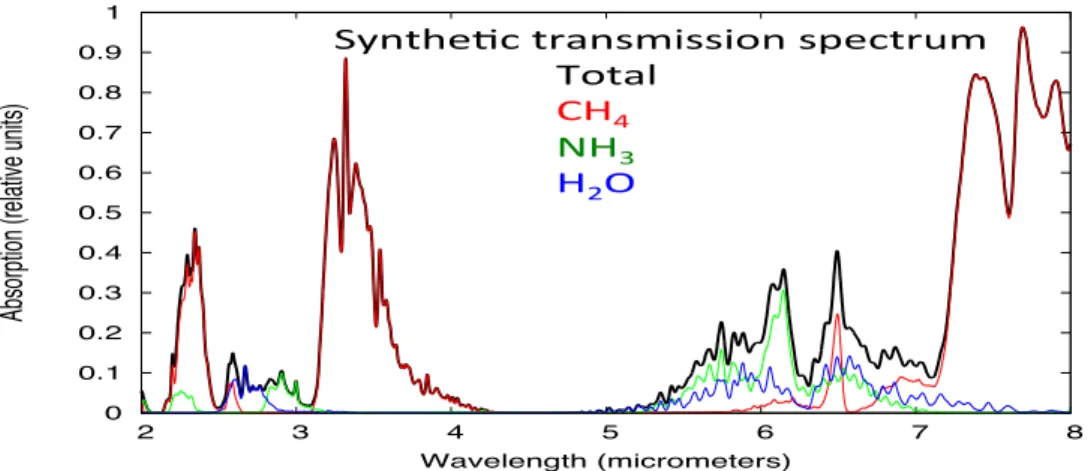
Our transmission spectra are generated using a line-by-line calculation of the absorption coefficient, assuming a single pressure layer (1 bar) and a single temperature (300 K). We use for NH3 a column density of 3 m-amagat, as measured in Jupiter in the 1.56-m
spectral window which probes down to a pressure of a few bars (Owen et al. 1977); we then derive column densities of 30 m-amagat for CH4 and 60 m-amagat for H2O,
respectively. Our transmission spectrum is convolved with a Gaussian function with a resolving power of 100 at 2 m, 200 at 4 m and 400 at 8 m. The resolution is comparable to the ARIEL one in the 2 – 4-m range and higher at 4 -8 m range, which allows a better description of the band shapes.
Figure 2 shows the synthetic transmission spectrum of a temperate Jupiter. For comparison, Figure 3 shows the synthetic spectrum of a cold Jupiter, where most of the water is trapped in the form of ice in the lower troposphere (in the gaseous phase, H2O:CH4:NH3 = 0.07:1:0.1). This corresponds to the spectrum of the actual Jupiter if it
were seen in transmission in front of the Sun.
Figure 2. A typical transmission spectrum for a temperate Jupiter (T = 350 K). Jupiter-like relative abundances are assumed for the molecules in the troposphere below the clouds, and no condensation is assumed for H2O: H2O:CH4:NH3 = 2.0:1.0:0.1. The full scale is equal to the amplitude of the transmission signal calculated in Table 2.
Total& CH4&
NH3&
Figure 3. A typical transmission spectrum for a cold Jupiter (T = 150 K). Jupiter-like relative abundances are assumed for the molecules in the troposphere, and condensation is assumed for H2O: H2O:CH4:NH3 = 0.07:1.0:0.1. The full scale is equal to the amplitude of the transmission signal calculated in Table 2.
Above the tropopause, other minor molecules are expected as products of photo-dissociation: C2H2 and C2H6 from the methane photo-dissociation, CO and CO2 from the
water photo-dissociation. By analogy with the case of Jupiter, we estimate the possible contribution due to photochemistry in the transmission spectrum by assuming the following abundances: (1) at P = 100 mb (tropopause), H2O:CH4:NH3 = 2:1:0.1 (as in the
troposphere); (2) in the stratosphere, at P = 1 mb, CH4:C2H2:C2H6 = 1:10-4:2 10-3, and
H2O:CO:CO2 = 1:1:0.2. Calculations show that CO and CO2 contribute as minor absorbers
in the infrared spectrum, while the contribution of hydrocarbons is negligible (Figure 4).
Figure 4. A typical transmission spectrum for a temperate giant exoplanet (T = 350 K), including the effect of photochemistry. Jupiter-like relative abundances are assumed for the molecules in the troposphere and no condensation is assumed (P = 100 mb, H2O:CH4:NH3 = 2.0:1.0:0.1). In the stratosphere (P = 1 mb), the relative abundances are H2O:CO:CO2 = 1:1:0.2. The contribution of hydrocarbons is negligible. The full scale is equal to the amplitude of the transmission signal calculated in Table 2.
!!!!CH4!
!!!!NH3!
!!!!H2O!
!!!!CO2!!CO!
What could be the condensates present in a temperate Jupiter? We know that hazes may be important contributors that flatten the infrared transmission spectrum of hot or warm exoplanets, as illustrated by the flat spectrum of GJ1214 b. For temperate objects colder than 500 K, all ices are in gaseous form. We can thus expect temperate Jupiters to be relatively free of condensates, as discussed by Sudarsky et al. (2000). Morley et al. (2012), however, have shown that some condensates (including Na2S, ZnS and KCl) might be present in the atmospheres of T-dwarfs, so the possible presence of clouds in temperate exoplanets is still an open question. In the lack of more information, we adopt in our study a low value of the albedo (0.03), as has been actually observed on hot Jupiters (Rowe et al. 2008).
Our analysis is consistent with the study of Sudarsky et al. (2000) who have characterized the various types of giant exoplanets as a function of their equilibrium temperature. Giant exoplanets in the 350 – 500 K range, as considered in the present study, are intermediate between Class II and Class III and show no NH3 nor H2O clouds;
they are supposed to have a very low albedo. The situation would be different for objects with an equilibrium temperature of 250 K (Class II), as the presence of a water cloud would lead to a high albedo. However, Class II objects are not considered in the present study because their expected transmission signal would be below the sensitivity limit of ARIEL (see Section 7).
4. Primary transit spectroscopy of a temperate Jupiter
Let us assume a Jupiter-size exoplanet transiting in front of its host star. During a primary transit, its atmosphere is observed in transmission at terminator in front of the stellar light. The area of planetary atmosphere observed in transmission is an annulus around the planet with a radial height of about 5 x H, where H is the scale height. H is equal to RT/μg, where R is the perfect gaz constant, T the temperature, μ the mean molecular weight of the atmosphere and g the planet's gravity. The amplitude of the absorption within the exoplanet’s atmosphere can be approximated as follows (Tinetti et al. 2013)
A = 5 x [2RpH/R*2] (6)
where Rp and R* are the radii of the planet and the star respectively.
For a hydrogen‐helium rich planet with μ = 2.4, the scale height (in km) can be expressed as
H = 3.46 x TP/g (7)
where TP is the equilibrium temperature of the exoplanet in Kelvins and g is the surface
gravity in m/s2 (at a pressure level of 1 bar). The surface gravity g can be expressed as
where MP and RP are the mass and the radius of the planet, expressed in Jovian masses
and radii, respectively. As a result, the amplitude of the absorption can be written (with R* expressed in solar radii):
A = 1.4 10-6x RP x H/R*2 (9)
For a hydrogen-rich exoplanet, we have
A = 1 .94 10-7 x T x RP3/MP/R*2 = 1.94 10-7 x T /R*2 (10)
where is the planet’s density, expressed in Jovian units. For hot Jupiters, typical values of A are a few 10-4. The amplitude of the signal is especially strong for planets having a
high temperature (and thus being close to their star), a large radius and a low molecular weight.
For a temperate Jupiter with an equilibrium temperature of 400 K around a solar-type star, we find A = 7.75 10-5. As compared with a hot Jupiter (T = 1600 K), the amplitude is
lower by a factor of 4 due to the low temperature. As compared with a super-Earth with a density equal of 4 times the Jovian value, with an effective temperature of 1600 K, the amplitude of a temperate giant exoplanet is expected to be of the same order. Temperate Jupiters could thus be considered to exist in the detectability range of ARIEL.
5. Secondary transit spectroscopy of a temperate Jupiter
Secondary transits provide a direct measurement of the dayside emission of the exoplanet. The ratio of the planet/star flux can be approximated as follows (Tinetti et al. 2013):
- in the visible and near-infrared range:
1 = [RP/R*]2 x [TP/T*]4 (11)
- in the mid and far-infrared (Rayleigh-Jeans approximation):
2 = [RP/R*]2 x [TP/T*] (12)
For a temperate Jupiter (T = 400 K), as compared to a hot Jupiter (T = 1600 K), 1 is lower by a factor 44 = 256, and 2 by a factor of 4. As compared with a hot super-Earth, 1 is lower by a factor of 10 and 2 larger by a factor of 7.5. These numbers show that, in the near-infrared range, temperate Jupiters are not suitable targets for secondary transit spectroscopy. The comparison would be more favorable for 2; however the Rayleigh-Jeans approximation holds only at long wavelengths (above about 20 m), and is not valid in the spectral range of ARIEL (2-8 m).
It can be noted that the secondary transit spectrum of a temperate Jupiter could be significantly more complex than the primary transit spectrum, for two reasons: (1) if a temperature inversion takes place above the tropopause, the bands of CH4, NH3 and H2O
C2H6) could have strong signatures in the mid-infrared, as observed in the case of solar
system giant planets.
In summary, we consider that, within the spectral range of ARIEL, temperate Jupiters are suitable targets for primary transit spectroscopy only.
6. How to optimize the primary transit spectroscopy of temperate Jupiters
We now consider temperate giant exoplanets orbiting low-mass stars. The advantage is twofold: (1) the amplitude of the primary transit signal is larger by a factor [1/R*]2
where R* is the radius of the star; (2) the revolution period is shorter than a year, which allows repeated transits of the object during the lifetime of the ARIEL mission.
For a star of mass M* and radius R* (in solar units) and effective temperature T* (in K), the star-planet distance D (in AU) of a fast-rotating exoplanet with an equilibrium temperature TP is given by the following equation:
D = [(1-a)0.25 x 279.0 (T*/5770)x R*0.5]/TP]2 (13)
or, using the equation
L* = 4T*4R*2 = (M*/Ms)3 (14)
D can also be expressed as:
D = [(1-a)0.25 x 279.0 (M*]3/4/TP]2 (15)
where a is the albedo of the planet and TP its equilibrium temperature; M*, R* and T*
are the mass, radius and effective temperature of the host star, expressed in solar units. In the case of a slow-rotating (tidally locked) planet, equations (13) an (15) become:
D = [(1-a)0.25 x 331.0 (T*/5770)x R*0.5]/TP]2 (16)
and
D = [(1-a)0.25 x 331.0 (M*]3/4/TP]2 (17)
Assuming for our exoplanet two possible values of TP (350 K and 500 K), we determine
in each case its distance to its host star D. For each spectral type, we consider the two cases (fast rotating or tidally locked object) and we compare the two values of D with Dsynch . It can be seen that the tidally locked regime is found for the M5 and M8 stars,
while fast-rotating objects are expected in all other cases. Then we calculate the revolution period P of the exoplanet, using the equation:
D3/P2 = M* (18)
We then calculate the amplitude of the transmission spectrum using Equation (9) for the two values of the exoplanet’s equilibrium temperature. The transit time t is estimated using the following equation:
t = [2R*/D] x P/2 (19)
with t expressed in hours, P in days, R* in solar radii, and D in AU, this equation becomes:
t = 0.0359 x R* x P /D (20)
Table 2
Estimated semi-major axis, rotational period, amplitude of primary transit signal and transit time for a Jovian-like exoplanet transiting around a star of spectral type between G2 and M8, using Equations (9), (13), (15), (16), (17), (18) and (20), with an albedo a = 0.03, assuming either a fast rotator (columns 6 and 8) or a tidally locked object (columns 7 and 9). Two cases are considered: TP = 350 K and TP = 500 K. The fast rotator case is
favored for G2 to M0 stars (M0 stars are actually an intermediate case); the tidally locked object case is favored for M5 and M8 stars.
Spectral type R (Rs) M (Ms) L (Ls) T* (K) D (AU) fast rot. D (AU) slow rot. P(d) fast rot. P(d) slow rot. A Transit time (h) G2 (TP= 350 K) G2 (TP= 500 K) 1.0 1.0 1.0 5770 0.625 0.306 0.880 0.431 180 61 301 103 6.78 10-5 9.69 10-5 10.3 7.1 G5 (TP= 350 K) G5 (TP= 500 K) 0.93 0.93 0.79 5641 0.561 0.274 0.790 0.386 159 54 266 91 7.84 10 -5 1.12 10-4 9.4 6.6 K0 (TP= 350 K) K0 (TP= 500 K) 0.85 0.78 0.40 4977 0.431 0.211 0.607 0.297 117 40 195 67 9.38 10-5 1.34 10-4 8.3 5.8 K5 (TP= 350 K) K5 (TP= 500 K) 0.74 0.69 0.16 4242 0.358 0.175 0.504 0.246 94 32 157 54 1.24 10 -4 1.77 10-4 7.0 4.9 M0(TP= 350 K) M0(TP= 500 K) 0.63 0.47 0.063 3642 0.201 0.099 0.282 0.139 48 17 80 28 1.71 10 -4 2.44 10-4 5.4 3.9 M5(TP= 350 K) M5(TP= 500 K) 0.32 0.21 0.008 3041 0.06 0.03 0.08 0.04 12 4 18 6 6.64 10 -4 9.50 10-4 2.6 1.7 M8(TP= 350 K) M8(TP= 500 K) 0.13 0.10 0.001 2691 0.02 0.01 0.03 0.015 3 1 6 2 3.98 10 -3 5.70 10-3 1.0 0.6 7. Sensitivity estimate
In order to estimate the observing time needed to obtain a transmission spectrum of a temperate Jupiter, we use as a calibrator the exoplanet WASP-76 b, for which a synthetic transmission spectrum is shown in the ARIEL proposal. This object has a mass of 0.92 MJ, a radius of 1.83 RJ, a temperature of 2200 K. The star WASP-76, of V magnitude 9.5,
located at 120 pc from the Sun, has a mass of 1.46 Ms, a radius of 1.73 Rs, and a temperature of 6250 K. The star-planet distance is 0.033 AU and the rotation period of the exoplanet is 1.81 days. The amplitude of primary transit is about 1.0 10-3. The time
transit is 3.4 hours. A summation of 25 transits (corresponding to 85 hours of total observing time) is needed to achieve a S/N of about 10.
We now estimate the number of transits needed for a temperate Jupiter around a M-dwarf to be observed by transmission spectroscopy with a total observing time of 100 hours. This corresponds to a S/N of about 12 for WASP-76 b, and about 2.5, 9.5 and 57 for temperate Jupiters around M0, M5 and M8 stars respectively. Table 3 summarizes the results. We also indicate the total time in orbit needed to accumulate the required
number of transits; this time must be shorter than the lifetime of the ARIEL mission of 4 years. The case of WASP-76 is added for comparison.
Table 3
Number of transits required to obtain 100 hours of integration time on a temperate Jupiter around a M star and total time required to accumulate these transits.
Spectral type R*(Rs) A S/N in
100 hours Period (d) t(h) Number of transits Total time needed for ttot = 100 h (d) WASP-76 1.73 1.0 10-3 12 1.81 3.4 30 54 M0(TP=350K) M0(TP=500K) 0.63 1.71 10-4 2.44 10-4 2 3 48 17 5.4 3.9 19 26 912 442 M5(TP=350K) M5(TP=500K) 0.32 6.64 10-4 9.50 10-4 8 11 18 6 2.6 1.7 38 59 684 354 M8(TP=350K) M8(TP=500K) 0.13 3.98 10-3 5.70 10-3 47 67 6 2 1.0 0.6 100 167 600 334
It can be seen that all three classes of objects can be considered within a lifetime of 4 years; however, temperate Jupiters around M5 to M8 dwarfs should be favored for a higher S/N ratio and a shorter required time of observation. As shown in Fig. 4, a signal-to-noise of 10 or higher with the resolving power of ARIEL (100 – 200) should be sufficient for separating the signatures of the main molecular species (H2O, CH4, NH3, CO,
CO2).
8. How to find exoplanets around M-dwarfs?
So far we know of no example of temperate Jupiters around M stars. Can we estimate the probability of finding such target in the coming decade? We know that M-dwarfs are dominant in stellar populations, however they are difficult to identify because of their low luminosity. According to some authors (Henry et al. 2002; Reylé 2006), 70% of these systems (corresponding to about 3000 samples) might exist remaining to be detected within 25 pc from the Sun. Several hundred of objects have already been found using the ground-based infrared surveys DENIS and 2MASS (Reylé 2006, Rajpurohit et al. 2014).
In addition, the CHEOPS, TESS and PLATO space missions are expected to provide new targets for transit spectroscopy. However, they will be oriented rather toward bright stars and small exoplanets. More importantly, the GAIA space mission is expected to bring an enormous database for this study. According to a simulation of stars observable with GAIA performed by Robin et al. (2014), a total of 1.3 107 stars with a visual
magnitude less than 12 (corresponding to the sensitivity limit of ARIEL) are expected to be observed by GAIA, including 11% of M-type stars. Knowing that about each star is expected to have a planet, the number of potential candidates is expected to be huge. In addition, GAIA will be able to perform photometry transits of Jupiter-like exoplanets around stars brighter than the 14th magnitude, including M-type stars.
It should be noted that transit spectroscopy around a M-dwarf star might be more difficult than around a G or K star, because of the intermittent flares emitted by these stars. However, the continuous near-infrared monitoring of the stellar flux by ARIEL, in parallel with the transit measurements, should make possible the identification and the removal of these anomalies.
Assuming M-stars can be found in sufficient numbers, one may question the probability of finding giant planets around such low-mass stars. We have no answer to this question yet, but some lessons can be drawn on the basis of the present exoplanet catalogs (Schneider, 2010). We know of about 150 exoplanets with masses greater than 10 jovian masses orbiting F, G or K stars, which seems to indicate that the mass ratio between a giant planet and its host star may actually be greater than the Jupiter/Sun mass ratio; a few examples of such objects can be found in Table 1. In addition, the recent detection of 7 planets in orbit around the ultra-cool M8 star TRAPPIST-1 (Gillon et al. 2017), possibly the result of a migration from beyond the ice line, may suggest that the presence of larger objects is also possible. In addition, the exoplanet demographics from microlensing suggest that giant planets around M-stars are more frequent than expected from radio-velocimetry studies, with a frequency of 0.11 for planets more massive than 50 terrestrial masses (Clanton and Gaudi, 2014).
9. Conclusion
In summary, it appears that temperate Jupiters orbiting M stars at semi-major axes between about 0.1 and 0.5 AU could be suitable targets for ARIEL. If such targets are identified in future surveys, their study with ARIEL would allow us to enlarge the range of physical atmospheric parameters to be covered, and thus to extend the exoplanets’ exploration by the mission.
References
Bolton, S. J. et al. 2017. Jupiter’s interior and deep atmosphere: The initial pole-to-pole passes with the Juno spacecraft. Science 356, 6340-6344
Clanton, C. and Gaudi, B. S. 2014. Synthetizing exoplanet demographics from radial velocity and microlensing surveys. II. The frequency of planets orbiting M-dwarfs. Astrophys. J. 791:91 (23pp)
Encrenaz, T. et al. 1999. The atmospheric composition and structure of Jupiter and Saturn from ISO observations: What have we learnt? Plan. Space Sci. 47, 1225-1242 Gillon, M. et al. 2017. Seven temperate terrestrial planets around the nearby utra-cool dwarf star TRAPPIST-1. Nature 542, 456-460
Grevesse, N., Asplund, M., Sauval, A.J., 2005. The new solar chemical composition. In: Alecian, G., Richard, O., Vauclair, S. (Eds.), Element Stratification of Stars, 40 years of Atomic Diffusion, EAS Publication Series, EDP Sciences.
Henry, T, Walkowicz, L. M., Barto, T. C., Golimowsky, D. A. 2002. Astron. J. 123, 2002 Kasting, J. F., Whitmire, D. P., and Reynolds, R. T. 1993. Habitable zones around main-sequence stars. Icarus 101, 108-128
Lainey, V. 2016. Quantification of tidal parameters from Solar system data.
Léger, A. et al. 2009. Transiting exoplanets from the CoRoT space mission. VIII CoRoT-7 b: the first super-Earth with measured radius. Astron. Astrophys. 506, 287-302
Morley, C. V. et al. 2012. Neglected clouds in T and Y dwarf atmospheres. Astrophys. J. 756:172(17pp)
Murray, C. D., Dermott, S. F. 2000. Solar system dynamics, Cambride University Press Owen, T. and Encrenaz, T. 2006. Compositional constraints on giant planet formation. Plan. Space Sci. 54, 1188-1196
Pollack, J. B. et al. 1996. Formation of the giant planets by concurrent accretion of solids and gas. Icarus 124, 62-85
Rajpurohit, A. S., Reylé, C., Allard, F. et al. 2013. Astron. Astrophys. 556, A15 Reylé C. 2006.Habilitation à Diriger des Recherches, Observatoire de Besançon. Robin A et al. 2004
Robin, A., Reylé, C., Luri, X. et al. 2014. Mem. S. A. It. 85, 560
Sudarsky, D., Burrows, A., Pinto, P. 2000. Albedos and reflection spectra of extrasolar giant planets. Astrophys. J. 588, 1121-1148
Tinetti, G. et al. 2011.The EChO Mission Proposal – A candidate for the ESA M3 mission Tinetti, G., Encrenaz, T., Coustenis, A. Spectroscopy of planetary atmospheres in our Galaxy. 2013. Astron. Astrophys. Rev. 21, 63