Evaluation of near-tropopause ozone distributions in the Global Modeling Initiative combined stratosphere/troposphere model with ozonesonde data

HAL Id: hal-00296537

https://hal.archives-ouvertes.fr/hal-00296537

Submitted on 6 May 2008

HAL is a multi-disciplinary open access

archive for the deposit and dissemination of

sci-entific research documents, whether they are

pub-lished or not. The documents may come from

teaching and research institutions in France or

abroad, or from public or private research centers.

L’archive ouverte pluridisciplinaire HAL, est

destinée au dépôt et à la diffusion de documents

scientifiques de niveau recherche, publiés ou non,

émanant des établissements d’enseignement et de

recherche français ou étrangers, des laboratoires

publics ou privés.

Global Modeling Initiative combined

stratosphere/troposphere model with ozonesonde data

D. B. Considine, J. A. Logan, M. A. Olsen

To cite this version:

D. B. Considine, J. A. Logan, M. A. Olsen. Evaluation of near-tropopause ozone distributions in

the Global Modeling Initiative combined stratosphere/troposphere model with ozonesonde data.

At-mospheric Chemistry and Physics, European Geosciences Union, 2008, 8 (9), pp.2365-2385.

�hal-00296537�

© Author(s) 2008. This work is distributed under the Creative Commons Attribution 3.0 License.

Chemistry

and Physics

Evaluation of near-tropopause ozone distributions in the Global

Modeling Initiative combined stratosphere/troposphere model with

ozonesonde data

D. B. Considine1, J. A. Logan2, and M. A. Olsen3 1_{NASA Langley Research Center, Hampton, Virginia, USA} 2_{Harvard University, Cambridge, Massachusetts, USA}

3_{Goddard Earth Sciences and Technology Center, University of Maryland, Baltimore County, Baltimore, Maryland, USA}

Received: 19 November 2007 – Published in Atmos. Chem. Phys. Discuss.: 29 January 2008 Revised: 15 April 2008 – Accepted: 18 April 2008 – Published: 6 May 2008

Abstract. The NASA Global Modeling Initiative has

de-veloped a combined stratosphere/troposphere chemistry and transport model which fully represents the processes govern-ing atmospheric composition near the tropopause. We evalu-ate model ozone distributions near the tropopause, using two high vertical resolution monthly mean ozone profile clima-tologies constructed with ozonesonde data, one by averag-ing on pressure levels and the other relative to the thermal tropopause. At the tropopause, model ozone is high-biased in the SH tropics and NH midlatitudes by ∼45% in a 4◦ lat-itude ×5◦ longitude model simulation. Doubling the res-olution to 2◦×2.5◦ increases the NH high bias to ∼60%, and reduces the tropical bias to ∼30%, apparently due to decreased horizontal transport between the tropics and ex-tratropics in the higher-resolution simulation. These ozone biases do not appear to be due to an overly vigorous resid-ual circulation, insufficient convection, or excessive strato-sphere/troposphere exchange, and so may be due to insuffi-cient vertical resolution or excessive vertical diffusion near the tropopause. In the upper troposphere and lower strato-sphere, model/measurement intercomparisons are strongly affected by the averaging technique.

Compared to the pressure-averaged climatology, NH and tropical mean model lower stratospheric biases are <20%. In the upper troposphere, the 2◦_×2.5◦_{simulation shows mean}

high biases of ∼20% and ∼35% during April in the trop-ics and NH midlatitudes, respectively. This apparently good

Correspondence to: D. Considine

(david.b.considine@nasa.gov)

model/measurement agreement degrades when relative-to-tropopause averages are considered, with upper troposphere high biases of ∼30% and 70% in the tropics and NH mid-latitudes. This occurs because relative-to-tropopause averag-ing better preserves the larger cross-tropopause O3gradients

which are seen in the daily sonde data, but not in daily model profiles. Relative-to-tropopause averages therefore more ac-curately reveal model/measurement discrepancies. The rela-tive annual cycle of ozone near the tropopause is reproduced very well in the model Northern Hemisphere midlatitudes. In the tropics, the model amplitude of the near-tropopause an-nual cycle is weak. This is likely due to the anan-nual amplitude of mean vertical upwelling near the tropopause, which anal-ysis suggests is ∼30% weaker than in the real atmosphere.

1 Introduction

The tropopause is surrounded by a transition region that is strongly influenced by both tropospheric and stratospheric processes (Holton et al., 1995; Wennberg, et al., 1998; Rood et al., 2000; Gettelman et al., 2004; Pan et al., 2004). It is a challenge to represent this “near-tropopause region” (NTR) in global models of atmospheric composition. Many mod-els do not consider all of the processes that influence the NTR, because they were designed for reasons of practicality and interest to focus on either the stratosphere or the tropo-sphere, but not both (e.g., Douglass and Kawa, 1999; Bey et al., 2001; Horowitz et al., 2003; Rotman et al., 2001).

Computational advances have allowed a class of compo-sition models to be developed recently that include both the

SONDE STATION LOCATIONS

Fig. 1. Geographic locations of the 23 ozonesonde stations used

in this study. Station names, latitudes and longitudes, and record length are given in Table 1.

stratosphere and the troposphere (e.g., Rotman et al., 2004; Chipperfield, 2006; Kinnison et al., 2007). The NASA Global Modeling Initiative (GMI) has constructed such a model (the Combo model), which includes a nearly complete treatment of both stratospheric and tropospheric photochem-ical and physphotochem-ical processes (Schoeberl et al., 2006; Ziemke et al., 2006; Duncan et al., 2007; Strahan et al., 2007). It uses the Lin and Rood (1996) transport scheme, which has been shown recently to be superior to spectral and semi-Lagrangian transport in representing the strong vertical tracer gradients that characterize the NTR (Rasch et al., 2006).

The Combo model has been shown to have many fa-vorable characteristics in the NTR, when it utilizes me-teorological data from a GCM. This includes good lower stratospheric transport (Douglass et al., 2003), and credible cross-tropopause mass and ozone fluxes (Olsen et al., 2004). Schoeberl et al. (2006) demonstrated that the Combo model reproduces the observed “tape recorder” characteristics of CO across the tropical tropopause. Strahan et al. (2007) showed that the model agrees well with many characteris-tics of satellite and aircraft observations of CO, O3, N2O,

and CO2in the lowermost stratosphere. They also found

re-alistic correlations between O3and CO near the extratropical

tropopause.

Ozone is an important species to represent well in the NTR, due to its central role in upper tropospheric chemistry (e.g., M¨uller and Brasseur, 1999), and its effect on the ra-diative balance of the atmosphere. Lacis et al. (1990) found the highest sensitivity of surface temperatures to changes in ozone near the tropopause, due to the large temperature con-trast between the NTR and the surface. Typically, modeled NTR ozone mixing ratios are substantially higher than ob-served, particularly just below the tropopause (e.g., Wauben et al., 1998; Rotman et al., 2004). This would obviously

overweight the radiative impact of the NTR on surface tem-peratures in chemistry-climate models with this defect.

Here we exploit the high vertical resolution of ozonesonde data to evaluate how well the GMI Combo model is able to reproduce NTR ozone distributions. We explore the mecha-nisms responsible for any deficiencies that we find. We focus on a climatological evaluation due to the GCM source of the meteorological data used to drive the GMI CTM. Following Logan (1999a), we construct climatological monthly average ozone profiles from the ozonesonde data. The 23-station cli-matology exploits the availability of a now-substantial num-ber of tropical sondes from the SHADOZ network (Thomson et al., 2003a) to more fully represent the tropics than has been previously possible. The number of sondes at each station is sufficient to define monthly means and medians precisely enough to allow an evaluation of the accuracy of the model results.

We also investigate the effects and importance of aver-aging relative to the tropopause versus averaver-aging at con-stant pressure levels to create the monthly profiles from daily ozonesondes. Averaging relative to the tropopause was shown by Logan (1999a) to substantially increase cross-tropopause vertical gradients in monthly averages. How this affects a model/measurement intercomparison has not yet been thoroughly investigated.

In Sect. 2 we describe the ozonesonde climatologies con-structed for this comparison. The GMI Combo model is de-scribed in Sect. 3. Section 4 presents comparisons between modeled distributions and the climatologies. We summarize these results and draw conclusions in Sect. 5.

2 Ozonesonde data set description

The ozonesonde data were analyzed in a manner similar to that described in Logan (1999a). She presented monthly av-erages for ozone on standard pressure levels, and on an al-titude grid relative to the height of the thermal tropopause. At the time, data were available for only two tropical sonde stations. Here we use data from 10 tropical stations in the Southern Hemisphere Additional Ozonesondes (SHADOZ) network (Thompson et al., 2003a), which started in 1998; two of these are in the northern hemisphere (NH). We use data from 12 extratropical stations in the NH. Station details are given in Table 1 and shown in Fig. 1.

The analysis was the same as that in Logan (1999a) with the following differences: the base period for the analysis was updated to 1985–2000 for the extratropical stations, and to all available data for the tropical stations, which have shorter records. The pressure levels were changed from irregular intervals (1000, 900, 800 hPa etc.) to 35 levels equally spaced in pressure altitude between 1000 and 5 hPa (∼1 km apart). Level averages were formed for each pressure level using all measurements within a month located within the pressure layer, with interpolation used only if there were

no measurements in a layer. This last change was made be-cause the data are now available with much higher vertical resolution than previously, when the poor resolution required that interpolation be used.

Exactly the same profiles were used to form the monthly means on the pressure levels and on the altitude grid rela-tive to the thermal tropopause. Some profiles were elimi-nated from the analysis as the tropopause levels derived from the temperature profiles were clearly unrealistic, as discussed in Logan (1999a). The data relative to the tropopause were interpolated to a grid with 1 km resolution in geometric al-titude, extending from 6 km below the tropopause to 12 km above it. These profiles were averaged together to produce monthly means relative to the tropopause, the RTT climatol-ogy. There are about 150 profiles in the monthly means for the European sonde stations, about 80 for the other extratrop-ical stations, and about 22 for the tropextratrop-ical stations.

Several factors motivated the choice to use the thermal tropopause as a reference. Temperature is simultaneously measured with ozone for each sonde, providing a straight-forward and high-resolution profile enabling accurate iden-tification of the thermal tropopause. Use of a dynami-cal tropopause definition based on potential vorticity (PV) would require interpolating relatively low vertical and hor-izontal resolution PV fields from one of several available analyzed data sets to the sonde profiles. Pan et al. (2004) found that the chemical transition layer surrounding the tropopause defined by CO and O3 correlations centered on

the thermal tropopause, also supporting the use of the ther-mal tropopause.

3 Model and run description

The GMI Combo model is described in Duncan et al. (2007) and Strahan et al. (2007). The basic structure of the Combo model, without photochemical modules, is also given in Con-sidine et al. (2005). Here, we present details salient to this study. The Combo model is an outgrowth of the original GMI model, a stratospheric CTM described in Rotman et al. (2001). The complete Combo model also includes a full treatment of both stratospheric and tropospheric photochem-istry. In this study, we run the Combo model at horizontal resolutions of 4◦ latitude by 5◦ longitude and 2◦ by 2.5◦. The model has 42 levels, extending from the surface up to 0.01 hPa. The resolution at the tropopause is about 1.1 km. This is comparable to other models of this type (e.g., Rot-man et al., 2004; Kinnison et al., 2007).

For this study, the Combo model was driven by meteo-rological data generated from a 50-year run of the GMAO GEOS4 AGCM (Bloom et al., 2005). This run was driven by observed sea surface temperatures, but was otherwise un-constrained. We use a 5-year subset corresponding to the years 1994–1998. The GEOS4 AGCM has both deep (Zhang

Table 1. Ozonesonde stations, locations, and data span. The table

gives the names of the stations providing data used in this paper, the geographic location of the station, and the span of time of observa-tions used in this paper.

Station Name Latitude Longitude Data Record

Resolute 75 −95 01/85–12/00 Churchill 59 −147 01/85–12/00 Goose Bay 53 −60 01/85–12/00 Edmonton 53 −114 01/85–12/00 Uccle 51 4 01/85–12/00 Hohenpeissenberg 48 11 01/85–12/00 Payerne 47 7 01/85–12/00 Sapporo 43 141 01/85–12/00 Boulder 40 −105 01/85–12/00 Wallops Island 38 −76 01/85–12/00 Tateno 36 140 01/85–12/00 Paramaribo 6 −55 09/99–12/04 Kuala Lumpur 3 102 01/98–12/04 San Cristobal −1 −90 03/98–12/04 Nairobi −1 37 09/97–12/04 Malindi −3 40 03/99–12/04 Natal −6 −35 01/98–12/04 Java −8 113 01/98–12/04 Ascension −8 −15 07/90–12/04 Samoa −14 −170 08/95–12/04 Fiji −18 178 02/97–12/04 Reunion Island −21 55 01/98–12/04 Pretoria −26 28 07/90–12/04

and McFarlane, 1995) and shallow (Hack, 1994) convective transport parameterizations.

The Combo model uses a 114-species chemical mecha-nism combining the stratospheric mechamecha-nism of Douglass et al. (2004) with the tropospheric chemical mechanism of Bey et al. (2001). Species transport is calculated using the flux-form semi-Lagrangian scheme of Lin and Rood (1996). The chemical mechanism describes both stratospheric halogen chemistry and tropospheric nonmethane hydrocarbon chem-istry, including isoprene oxidation (Horowitz et al., 1998). Both stratospheric and tropospheric heterogeneous reactions are included in the chemical mechanism. PSCs are parame-terized using the scheme of Considine et al. (2000). Tropo-spheric heterogeneous reactions occur on tropoTropo-spheric sul-fate, dust, sea-salt, and organic and black carbon aerosol dis-tributions generated by the Goddard Chemistry, Aerosol, Ra-diation and Transport model (Chin et al., 2002).

Mixing ratio boundary conditions for stratospheric source gases, N2O, and CH4correspond to the mid-1990’s. Surface

emission inventories are described in Bey et al. (2001) and Duncan et al. (2003), and represent rates typical of the mid-1990’s. Lightning NOx is also included as monthly mean

emissions fields. The lightning source is 5.0 Tg N/y. The horizontal distribution of lightning emissions is based on the

TOMS 94-98 COLUMN O₃ 0 2 4 6 8 10 12 -90 -60 -30 0 30 60 90 L A T IT U D E 0 2 4 6 8 10 12 -90 -60 -30 0 30 60 90 L A T IT U D E TOMS 94-98 COLUMN O₃ 200 220240 260 260 260 280 280 280 300 300 300 300 320 320 340 340 360 38 0 400 MODEL 94-98 COLUMN O₃ 0 2 4 6 8 10 12 -90 -60 -30 0 30 60 90 L A T IT U D E 0 2 4 6 8 10 12 -90 -60 -30 0 30 60 90 L A T IT U D E MODEL 94-98 COLUMN O₃ 180 200220 240 240 240 240 240 260 260 260 260 280 280 280 280 280 300 300 300 320 320 340 360 380 MODEL-TOMS COLUMN O₃ 0 2 4 6 8 10 12 MONTH OF YEAR -90 -60 -30 0 30 60 90 L A T IT U D E 0 2 4 6 8 10 12 MONTH OF YEAR -90 -60 -30 0 30 60 90 L A T IT U D E MODEL-TOMS COLUMN O₃ -30 -25 -25 -25 -20 -20 -20 -20 -15 -15 -15 -15 -15 -15 -15 -10 -1₀ -10 -10 -5 -5 0 0 5 5 ₁₀₁₅

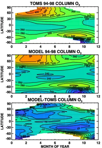
Fig. 2. Top panel: 1994–1998 average zonal mean total ozone from

the Total Ozone Mapping Spectrometer merged ozone dataset, as function of time of year and latitude. Middle panel: 1994–1998 average zonal mean total ozone from the GMI combined model, as function of time of year and latitude. Bottom panel: Model – observed differences, in Dobson units.

ISCCP deep convective cloud climatology as described in Price et al. (1997). Lightning flash rates are from Price and Rind (1992), and the vertical distribution of lightning NOxis

based on the cloud resolved convection simulations of Pick-ering (1998).

The initial condition was taken from a 10-year spinup run of the Combo model, which is enough time for strato-spheric species to converge to an approximate annually re-peating steady-state condition well above the lower strato-sphere, the focus of this study. Diurnal average 3-D gridded ozone distributions were output daily. These were interpo-lated to the ozonesonde station locations, and used to con-struct the monthly average profiles we compare to observa-tions in the next section.

HALOE 94-98 PROFILE O

, APR

-60 -45 -30 -15 0 15 30 45 60 75 100 10 1 PR ESSU R E (h Pa ) -60 -45 -30 -15 0 15 30 45 60 75 100 10 1 PR ESSU R E (h Pa )

HALOE 94-98 PROFILE O

, APR

1 1 2 2 2 ₂ 3 3 3 3 4 4 4 ₄ 5 5 5 6 6 6 7 7 8 8 9 10

94-98 AV MODEL PROFILE O

, APR

-60 -45 -30 -15 0 15 30 45 60 75 100 10 1 PR ESSU R E (h Pa ) -60 -45 -30 -15 0 15 30 45 60 75 100 10 1 PR ESSU R E (h Pa )

94-98 AV MODEL PROFILE O

, APR

1 1 2 2 2 2 3 3 3 ₃ 4 4 4 4 5 5 5 6 6 6 7 7 8 8 9 10

94-98 AV O

% DIFF, APR

94-98 AV O

% DIFF, APR

Fig. 3. Top panel: Zonal mean ozone distribution from version 19

Halogen Occultation Experiment (HALOE) data gathered during April for the years 1994–1998, as function of latitude and pressure in hPa. Middle panel: GMI combined model zonal mean ozone, av-eraged for Aprils from 1994–1998 as function of latitude and pres-sure. Bottom panel: Percent difference of April zonal mean mod-eled ozone distribution from observed ozone distribution, in per-cent. Contour levels: 0%, ± 10%, ± 20%, . . ..

4 Results

4.1 Global comparisons

We first provide a global-scale perspective for subsequent comparisons with the ozonesonde climatologies. Fig-ure 2 compares model column ozone distributions from the 2◦_×2.5◦ _{model run throughout the year with 1994–}

1998 average column ozone from the merged Total Ozone Mapping Spectrometer (TOMS)/Solar Backscatter Ultravio-let (SBUV) measurement data set (Stolarski and Frith, 2006). The model reproduces well the observed average global total ozone distribution during this time period. The annual cy-cle of tropical total ozone is represented well, though model values are about 20 DU low compared to the TOMS observa-tions. The model NH springtime peak of ∼400 DU is a few DU low, occurs ∼2 weeks early, and is not distinctly off the

Resolute (-95, 75)

Goose_Bay (-60, 53)

Edmonton (-114, 53)

Wallops_Island (-76, 38)

Payerne (7, 47)

Sapporo (141, 43)

San_Cristobal (-90, -1)

Nairobi (37, -1)

Fiji (178, -18)

Fig. 4. Comparison of GMI combined model (red lines) and observed (black lines) monthly mean (solid lines) and median (dashed lines)

tropopause pressures as function of time of year at six Northern Hemisphere stations and three stations in the Southern Hemisphere tropics. Vertical bars on model mean indicate ± two times standard error of the monthly mean values. Note inverted pressure axis. The station name and location is given in title of each panel of the figure.

pole as is the case with the observations. The NH high lati-tude summertime ozone decrease is reproduced well. In the SH, the model area over 340 DU is smaller than observed, resulting in model O3about 25 DU low, but is otherwise in

good agreement. The model produces a slightly weaker but well-timed ozone hole. Low model values at high latitudes during the SH summer suggest a somewhat too-isolated SH polar region during the spring and summer. Since total ozone

is very sensitive to the stratospheric residual circulation, the good agreement between observed and modeled total ozone, in particular the lack of a strong latitudinal gradient in model differences from observations shown in the third panel of Fig. 2, suggests that the stratospheric residual circulation of the GEOS-4 AGCM is fairly realistic.

Figure 3 compares the model zonal mean distribution of stratospheric ozone in April from the 2◦×2.5◦ model run

with observations made during April by the Halogen Oc-cultation Experiment (HALOE) on board the Upper Atmo-sphere Research Satellite (UARS) between 1994 and 1998 (Russell et al., 1993). The figure shows excellent correspon-dence between the observations and the model throughout most of the stratosphere. The model is generally within 10% of observations. There is a high-bias of up to 30% in the trop-ical lower stratosphere compared to HALOE observations, which will be discussed further below. Overall, the compar-ison reveals no serious deficiencies in the model representa-tion of stratospheric ozone distriburepresenta-tions.

The 4◦×5◦ model run also compares very well with the merged total ozone and HALOE data (not shown). The dif-ferences that exist, such as a shallower ozone hole and some-what larger model high-biases in the tropical lower strato-sphere, are generally minor in this global perspective. 4.2 Tropopause heights

As a test of model meteorological characteristics in the NTR, we first compare modeled and observed thermal tropopause heights at selected stations in Fig. 4. As we discuss in Sec-tion 2 above, we use the thermal tropopause because high vertical resolution temperature data for each ozonesonde is available which allows the thermal tropopause to be reliably identified. The observed tropopause values in Fig. 4 are from the RTT climatology, not the pressure-averaged climatology, calculated as described in Sec. 2. To find the tropopause height for a model daily profile, we first interpolated the pro-file to a 0.1 km grid using cubic splines and then applied the WMO (1957) criterion for tropopause height. The cor-responding pressure values were combined to construct the monthly means and medians shown in Fig. 4. Solid lines show monthly mean values, dashed lines show monthly me-dians. Fig. 4 includes ±2σ standard error bars for both mod-eled and observed values. These indicate that the means and medians have been defined precisely enough for meaning-ful comparisons. (Note that the smallness of the model er-ror compared to the erer-ror in the sonde climatology does not reflect differences in variability, which is comparable to ob-servations, but is due to the typically larger number of model values used to calculate the means and medians.) The sta-tions were chosen to span the latitude range of the obser-vations and show typical results. The differences between monthly mean and median tropopause heights are small at all stations in both the observations and the model. There is good agreement between modeled and observed tropopause pressures, including the annual cycle. Differences are largest at Resolute (75◦N) and at Wallops Island (38◦N).

Table 2 provides a summary of the comparisons for all sta-tions. The model tropopause is typically at slightly lower pressures than observed, except for Uccle, Paramaribo, Java, and Reunion Island. There is anomalously poor agreement at Tateno (36◦N), with model pressures ∼21% lower than observations. This is primarily a consequence of

tempera-ture profiles with double tropopauses, which sometimes oc-cur near the subtropical jet. Due to this poor agreement, we exclude Tateno from further analysis.

4.3 Tropopause ozone

Figure 5 compares for the 4◦×5◦model run the annual cy-cle of observed monthly mean tropopause ozone (black line) with model monthly mean tropopause ozone (red line) and model ozone values sampled at observed tropopause alti-tudes (blue line). Ozone at the model tropopause is higher than observed values, both in the tropics and NH extratrop-ics and throughout the year. Figure 5 shows that the model high bias is occasionally due simply to a higher tropopause in the model than observations – for instance, at Resolute af-ter March. However, at most other locations model ozone is high-biased even at the observed tropopause. Figure 5 also shows that the annual cycle of model tropopause ozone is generally similar in phasing to the observations. The ab-solute magnitude of the annual cycle in the model at these locations is also similar to the observations, though in per-centage terms the annual cycles are somewhat weaker than is observed.

Figure 6 shows results for the 2◦×2.5◦ run. The tropopause ozone bias in the extratropics is largest during the spring and summer. At Resolute, Goose Bay, and Edmonton, peak ozone values are about 75 ppbv higher than the 4◦×5◦ run. At Payerne and Sapporo, there are smaller increases of ∼30 ppbv. The tropical stations show a smaller ozone high bias compared to the 4◦×5◦run.

Figure 7 shows the percent difference between modeled and observed annually averaged tropopause ozone for all sta-tions, as a function of station latitude. Results for both the 4◦_×5◦ _{and 2}◦_×2.5◦ _{model runs are shown. In the}

extrat-ropics (38◦_–75◦_{N), where annual mean tropopause ozone is}

116–149 ppbv, the model has a high bias of 36–72% in the 4◦×5◦ run (mean 45%). The extratropical high bias in the 2◦×2.5◦model run is significantly larger, with the mean bias increasing to ∼61%. However, there are reductions for Boul-der and Wallops Island, the two lowest-latitude midlatitude stations considered. In the tropics, observed annual mean tropopause ozone is 58–130 ppbv. The 4◦×5◦ run shows a high bias of 17–63% (mean 43%) in the tropics. This drops to ∼31% in the 2◦×2.5◦model run.

The fact that model tropopause high biases are larger in the 2◦_×2.5◦ _{run at midlatitude stations, and smaller in the}

tropics, may be explained by lower effective horizontal dif-fusion in the higher resolution run. Strahan and Polan-sky (2006) showed that simulations at 2◦×2.5◦ better re-solved the stratospheric subtropical and polar mixing bar-riers, leading to larger horizontal gradients and improving the simulation of stratospheric dynamical features. Reduced horizontal mixing between the tropics and the midlatitudes would tend to decrease tropical mixing ratios and increase those at mid and higher latitudes. Thus, the improved model

Resolute (-95, 75)

Goose_Bay (-60, 53)

Edmonton (-114, 53)

Wallops_Island (-76, 38)

Payerne (7, 47)

Sapporo (141, 43)

San_Cristobal (-90, -1)

Nairobi (37, -1)

Fiji (178, -18)

Fig. 5. Comparison of annual cycle of GMI Combo model monthly mean tropopause ozone (red lines), Combo model ozone at the observed

tropopause (blue lines), and observed tropopause ozone (black lines) at six Northern Hemisphere stations and three stations in the Southern Hemisphere tropics. Ozone units are parts per billion by volume. The vertical bars on the lines indicate ±2 times the standard error. Model

resolution is 4◦×5◦.

resolution appears to have removed an error (high horizontal diffusivity) that was compensating for a second error which is responsible for high biases at the extratropical model tropopause.

A possible explanation for the ozone high bias at the tropopause seen in both simulations is an overly vigor-ous residual circulation in the GEOS 4 AGCM. Strahan et al. (2007) found overly strong ascent and mixing in the

GEOS 4 AGCM tropical lower stratosphere, particularly dur-ing the fall, suggestdur-ing that the residual circulation may be too strong. Since according to Olsen et al. (2007) the residual circulation is strongly correlated with stratosphere-troposphere exchange, we performed linear regressions of the 60 (5 years at 12 months/year) zonal mean, monthly mean O3values at each NH latitude and pressure level in the 4◦×5◦

Resolute (-95, 75)

Goose_Bay (-60, 53)

Edmonton (-114, 53)

Wallops_Island (-76, 38)

Payerne (7, 47)

Sapporo (141, 43)

San_Cristobal (-90, -1)

Nairobi (37, -1)

Fiji (178, -18)

Fig. 6. Same as Fig. 5, except for 2◦×2.5◦run.

NH extratropical cross-tropopause O3flux, calculated as

de-scribed in Olsen et al. (2004). (Briefly, the O3flux across

the tropopause is calculated as the difference between the flux crossing the 380 K potential temperature surface and the change in O3in the lowermost stratosphere.) From these

re-gressions we calculated at each latitude and pressure level the linear correlation and fractional sensitivity (percent change in O3 per percent change in flux) of zonal mean, monthly

mean O3with the monthly mean NH cross-tropopause flux

of O3. This is shown in Fig. 8. The top panel of Fig. 8

shows that O3near the tropopause is strongly positively

cor-related with STE poleward of ∼30◦_{. (Note that for 60 points,}

the probability that a correlation of more than 0.5 occurs by chance is less than 0.05%). The correlation remains high throughout most of the extratropical stratosphere. The bot-tom panel suggests that a 1% increase in STE results in an ∼0.5–0.6% increase in tropopause O3. Given the NH mean

high bias of ∼45%, Fig. 8 suggests that a reduction in STE of ∼90% would be required to eliminate the model high bias at the tropopause in the NH.

Model stratosphere-to-troposphere exchange of NH extra-tropical O3in the 4◦×5◦run is 266±9 Tg yr−1, which agrees

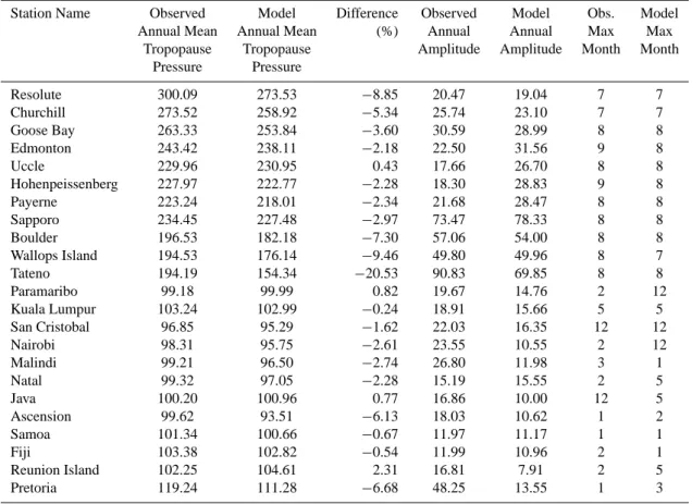
Table 2. Characteristics of observed and modeled thermal tropopause heights at observation locations. Column 1: Observed annual mean

tropopause pressure, in hPa. Column 2: Model annual mean tropopause pressure, in hPa. Column 3: percent difference of model from observed annual mean tropopause pressure. Columns 4 and 5: Amplitude of observed and modeled annual cycles, respectively, as percent of annual mean value. Columns 6 and 7: Observed and modeled month of minimum tropopause pressure (maximum tropopause altitude).

Station Name Observed Model Difference Observed Model Obs. Model

Annual Mean Annual Mean (%) Annual Annual Max Max

Tropopause Tropopause Amplitude Amplitude Month Month

Pressure Pressure Resolute 300.09 273.53 −8.85 20.47 19.04 7 7 Churchill 273.52 258.92 −5.34 25.74 23.10 7 7 Goose Bay 263.33 253.84 −3.60 30.59 28.99 8 8 Edmonton 243.42 238.11 −2.18 22.50 31.56 9 8 Uccle 229.96 230.95 0.43 17.66 26.70 8 8 Hohenpeissenberg 227.97 222.77 −2.28 18.30 28.83 9 8 Payerne 223.24 218.01 −2.34 21.68 28.47 8 8 Sapporo 234.45 227.48 −2.97 73.47 78.33 8 8 Boulder 196.53 182.18 −7.30 57.06 54.00 8 8 Wallops Island 194.53 176.14 −9.46 49.80 49.96 8 7 Tateno 194.19 154.34 −20.53 90.83 69.85 8 8 Paramaribo 99.18 99.99 0.82 19.67 14.76 2 12 Kuala Lumpur 103.24 102.99 −0.24 18.91 15.66 5 5 San Cristobal 96.85 95.29 −1.62 22.03 16.35 12 12 Nairobi 98.31 95.75 −2.61 23.55 10.55 2 12 Malindi 99.21 96.50 −2.74 26.80 11.98 3 1 Natal 99.32 97.05 −2.28 15.19 15.55 2 5 Java 100.20 100.96 0.77 16.86 10.00 12 5 Ascension 99.62 93.51 −6.13 18.03 10.62 1 2 Samoa 101.34 100.66 −0.67 11.97 11.17 1 1 Fiji 103.38 102.82 −0.54 11.99 10.96 2 1 Reunion Island 102.25 104.61 2.31 16.81 7.91 2 5 Pretoria 119.24 111.28 −6.68 48.25 13.55 1 3

well with several other estimates (Olsen et al., 2004). A 90% reduction is therefore unreasonable. Changes to the resid-ual circulation of the magnitude necessary to reduce STE by 90% would also adversely affect the good agreement of stratospheric O3 with observations shown in Figs. 2 and 3,

in addition to increasing the tropical tropopause ozone high bias. Thus Fig. 8 does not support the idea that the ozone high biases at the model tropopause can be explained simply by an overly vigorous residual circulation and consequently too much STE. Additional evidence for the soundness of the GEOS4 AGCM meteorological data is provided in Strahan et al. (2007), which demonstrates that transport processes connecting the tropical lower and upper troposphere, and be-tween the tropical UT and the extratropical lowermost strato-sphere are represented correctly.

Other possible contributors to the model high bias in-clude insufficient convection, insufficient vertical resolution at the tropopause and an overly vertically diffusive transport scheme. We tested the effects of model convective processes by conducting a simulation with convection turned off. This only increased tropopause O3values by ∼5% in the

extrat-ropics, and ∼10% in the textrat-ropics, indicating that insufficient convection is not a likely explanation. Rasch et al. (2006) demonstrated that the Lin and Rood transport scheme used in the Combo model is substantially less vertically diffusive than other popular schemes for simulating tracer transport in the NTR. Thus it is most likely that higher vertical resolu-tion in the NTR is necessary to eliminate the high bias of tropopause ozone.

4.4 Effects of averaging method on ozone gradients In making comparisons of the observed and modeled ver-tical distribution of ozone, we consider two approaches: a pressure coordinate and a vertical coordinate defined rela-tive to the tropopause. We illustrate the differences between the two averaging methods in Fig. 9. Figure 9a shows as a function of pressure the 49 sonde profiles in the clima-tologies sampled at Edmonton for Januarys between 1985 and 2000 (red lines), the monthly average vertical profile averaged at constant pressure levels, and one standard de-viation error profiles (black lines). The figure shows that

TROPOPAUSE O

DIFF (%)

Fig. 7. Percent difference between modeled and observed annually

averaged tropopause ozone for all stations, as a function of station

latitude. Red asterisks show results from 4◦×5◦run, blue diamonds

show results from 2◦×2.5◦run.

tropopause pressures (black crosses) are spread over the re-gion within about one half of an e-fold of the monthly me-dian tropopause pressure. Figure 9b shows the same pro-files in a RTT coordinate system, as well as the monthly mean profile averaged in RTT coordinates along with the plus and minus standard deviations. It is obvious that the profiles are more organized in Fig. 9b compared to Fig. 9a, especially near the tropopause, because a substantial fraction of the variability is related to daily changes in tropopause height. Fig. 9c compares the monthly average profiles and the standard deviations shown in Fig. 9a and b. It is impor-tant to note that to plot the RTT-average profile as a func-tion of pressure in Fig. 9c, we have normalized the RTT-average profile relative to the monthly median tropopause pressure. Figure 9c illustrates that pressuaveraging re-sults in weaker cross-tropopause gradients and larger UT ozone mixing ratios than the RTT-averaged values near the tropopause. RTT-averaging also reduces the variability near the tropopause. Figure 9d shows the percent deviation of the pressure-averaged profile from the RTT-averaged profile. Differences peak in the UT, with pressure averaged values up to 40% higher than RTT-averaged results.

Figure 10 shows model ozone profiles at Edmonton. (Re-sults from the 2◦×2.5◦run are shown, but there is little dif-ference between the two resolutions.) Figure 10a shows that model tropopause pressure variablity is similar to observa-tions (the standard deviation of the model tropopause pres-sure at Edmonton during January is ∼20% smaller than ob-servations). As is observed, the RTT-averaged profiles shown

O3 CORR WITH STE VARIABILITY

0 15 30 45 60 75 90 LATITUDE 1000 100 10 PR ESSU R E (h Pa ) 0 15 30 45 60 75 90 LATITUDE 1000 100 10 PR ESSU R E (h Pa )

O3 CORR WITH STE VARIABILITY

-0.6 -0.5_-0.4 -0.3-0.2 -0.2 -0.1 -0.1 -0.1 0 .0 0.0 0.0 0.0 0.1 0.1 0.1 0 .2 0.2 0.2 0 .3 0.3 0.3 0 .4 0.4 0.4 0 .5 0.5 0.5 0.5 0.5 0.6 0.6 0.6 0.6 0.6 0.7 0.7 0.7 0.7 0.7 0.8 0.8 0.8 0.8 0.8 0.8 0.9

FRACTIONAL SENSITIVITY OF O3 TO STE

0 15 30 45 60 75 90 LATITUDE 1000 100 10 PR ESSU R E (h Pa ) 0 15 30 45 60 75 90 LATITUDE 1000 100 10 PR ESSU R E (h Pa )

FRACTIONAL SENSITIVITY OF O3 TO STE

-0.3_-0.2 -0.1 0 .0 0.0 0.0 0.0 0.1 0.1 0.1 0.1 0.1 0.2 0.2 0.2 0.2 0.2 0.3 0.3 0.3 0.3 0.4 0.4 0.5 0.5

Fig. 8. Top panel: Distribution of linear correlation coefficients

produced by regressing the monthly mean, zonal mean O3 at

each latitude and pressure level in the 4◦×5◦run of the Combo

model with the monthly mean cross-tropopause flux of O3in the

NH extratropics. Bottom panel: Fractional sensitivity of monthly

mean, zonal mean O3in the 4◦×5◦ run to changes in the

cross-tropopause flux of O3in the NH extratropics. Fractional

sensitiv-ity is defined as the fractional change in O3mixing ratio per

frac-tional change in the monthly mean cross-tropopause flux of O3, or

S=m×<FNH>/<O3>, where m is the slope of the linear

regres-sion, <O3>is the mean monthly mean, zonal mean O3over the

5-year model integration at some latitude and pressure, and <FNH>

is the 5-year mean NH O3flux.

in Fig. 10b are more organized than in Fig. 10a. Unlike the observations, Fig. 10c shows similar but smaller differences between pressure averaging and RTT-averaging, both in the change in upper tropospheric ozone values and profile vari-ability. Figure 10d shows that the percent deviation of the pressure-averaged profile from the RTT-averaged profile is ∼8%, smaller than the observed ∼40% difference shown in Fig. 9d.

The results shown in Figs. 9d and 10d are typical at other locations and times of year. Model discrepancies between the two averaging techniques are generally small, while the differences between observed profiles averaged using these two techniques are much larger. Logan (1999a) showed that the vertical gradient in monthly averaged ozone profiles

con-PRESS AV SONDE O3, JAN 10 100 1000 MIXING RATIO (PPBV) -1 -.75 -.5 -.25 0 .25 .5 .75 1 PR ESS R EL T O T R O P (EF O L D ) 92 119 152 195 251 322 414 531 682 a

RTT AV SONDE O3, JAN

10 100 1000 MIXING RATIO (PPBV) -1 -.75 -.5 -.25 0 .25 .5 .75 1 F R A C O F T R O P PR ESS (EF O L D ) b PRESSURE AND RTT AV O3 10 100 1000 MIXING RATIO (PPBV) -1 -.75 -.5 -.25 0 .25 .5 .75 1 PR ESS R EL T O T R O P (EF O L D ) 92 119 152 195 251 322 414 531 682 c PRESS AV - RTT AV, % -60 -40 -20 0 20 40 60 PERCENT DIFF -1 -.75 -.5 -.25 0 .25 .5 .75 1 PR ESS R EL T O T R O P (EF O L D ) 92 119 152 195 251 322 414 531 682 d

Fig. 9. (a) Daily ozonesonde profiles at Edmonton (red lines),

plot-ted as function of pressure, for Januarys between 1985 and 2000. Left axis shows fraction of pressure efold from monthly median tropopause pressure. (The vertical axis is marked by the exponent y, where y varies over the range (−1,1), and the pressure is given

by Ptropey). Right axis indicates pressure in hPa. Black crosses

indicate thermal tropopause pressures for each profile. Black solid line is monthly mean ozone profile averaged as function of pres-sure. Black dashed lines indicate ± one standard deviation. (b) Red lines show ozonesonde profiles at Edmonton in January, plot-ted as fraction of efold of each profile’s tropopause pressure. (The vertical axis is marked by the exponent y, which varies over the

range e1 to e−1.) Black crosses indicating the tropopause now

all lie at y=0. Black solid profile shows monthly average at

con-stant fraction of tropopause pressure. Black dashed lines

indi-cate ± one standard deviation. (c) Comparison of monthly aver-aged profiles using pressure averaging (red lines) and relative-to-tropopause averaging (blue lines). Vertical axis is pressure. The relative-to-tropopause profile is plotted relative to the monthly me-dian tropopause height. (d) Percent difference of pressure-averaged from RTT-averaged profiles.

structed from sondes is on the order of a factor of 2 steeper when averaged relative to the tropopause. Here, we see that the model does not correctly reproduce the atmosphere in this regard. As a result, good agreement between mod-eled and observed pressure-averaged results does not imply good correspondence between modeled and observed cross-tropopause O3 profiles. Comparing RTT averages should

provide a more accurate picture of the discrepancies between the model and observations.

We suggest an explanation of the model insensitivity to averaging technique, with the following heuristic example: Presume that the ozone change in the model between its characteristic stratospheric and tropospheric values is given by 1O3, and the characteristic vertical depth of the region

over which the transition from stratospheric to tropospheric O3values occurs is given by the distance 1zNTR. Then the

ozone gradient across this region in a daily ozone profile is just S=1O3/1zNTR. We assume that this transition region

Edmonton (-114, 53) JAN 10 100 1000 MIXING RATIO (PPBV) -1 -.75 -.5 -.25 0 .25 .5 .75 1 PR ESS R EL T O T R O P (EF O L D ) 93 120 154 197 253 325 417 536 688 a Edmonton (-114, 53) JAN 10 100 1000 MIXING RATIO (PPBV) -1 -.75 -.5 -.25 0 .25 .5 .75 1 F R A C O F T R O P PR ESS (EF O L D ) b Edmonton (-114, 53) JAN 10 100 1000 MIXING RATIO (PPBV) -1 -.75 -.5 -.25 0 .25 .5 .75 1 PR ESS R EL T O T R O P (EF O L D ) 93 120 154 197 253 325 417 536 688 c Edmonton (-114, 53) JAN -10 -5 0 5 10 PERCENT DIFF -1 -.75 -.5 -.25 0 .25 .5 .75 1 PR ESS R EL T O T R O P (EF O L D ) 93 120 154 197 253 325 417 536 688 d

Fig. 10. Same as Fig. 9, except for the 155 daily GMI Combo model

January profiles produced during the 1994–1998 model run.

will move up and down in altitude over the course of a month as the tropopause height varies. We label the characteristic variation in the height of the tropopause as 1zTROP. Now,

the RTT monthly average will by definition be insensitive to this movement, so we will just have: <S>RTT∼S. However,

the tropopause height variability will smear the gradient in a pressure average, as each daily profile is shifted up or down by the movement of the tropopause. This results in a pressure-averaged mean slope of: <S>PRESS∼1O3/

(1zNTR+1zTROP)=<S>RTT×1zNTR/(1zNTR+1zTROP).

This equation suggests that the larger the size of the tran-sition region between the troposphere and stratosphere (1zNTR)relative to the monthly variability of the tropopause

height (1zTROP), the smaller the difference between RTT

and pressure averaging. Thus the weakness of the model daily profile vertical gradients shown in Fig. 10b can produce a smaller than observed sensitivity to the averaging technique. The equation also suggests that overly weak tropopause pressure variability could result in low sensi-tivity to averaging technique. However, the ∼20% weaker tropopause height variability seen in the model is not large enough to account for the much weaker model sensitivity to averaging technique compared to observations.

4.5 Profile ozone comparisons

Figure 11 shows 2◦_×2.5◦_{run profile comparisons with}

ob-servations of ozone mixing ratios from a pressure of half an efold below the observed monthly median tropopause pres-sure to half an efold above at Resolute, Hohenpeissenberg, and Ascension. Shown are model RTT-averaged monthly mean profiles, plotted relative to the model monthly median tropopause (red), and relative to the observed monthly me-dian tropopause (green). Plotting relative to the observed monthly median tropopause allows comparison of modeled

Resolute (-95, 75) JAN 100 1000 MIXING RATIO (PPBV) -.5 -.25 0 .25 .5 PR ESS R EL T O T R O P (EF O L D ) 175 225 289 371 476 Hohenpeissenberg (11, 48) JAN 100 1000 MIXING RATIO (PPBV) -.5 -.25 0 .25 .5 136 174 224 288 369 Ascension (-15, -8) JAN 100 1000 MIXING RATIO (PPBV) -.5 -.25 0 .25 .5 55 71 91 117 150 PR ESSU R E (h Pa ) Resolute (-95, 75) APR 100 1000 MIXING RATIO (PPBV) -.5 -.25 0 .25 .5 PR ESS R EL T O T R O P (EF O L D ) 197 252 324 416 534 Hohenpeissenberg (11, 48) APR 100 1000 MIXING RATIO (PPBV) -.5 -.25 0 .25 .5 147 189 242 311 400 Ascension (-15, -8) APR 100 1000 MIXING RATIO (PPBV) -.5 -.25 0 .25 .5 57 73 94 121 155 PR ESSU R E (h Pa ) Resolute (-95, 75) JUL 100 1000 MIXING RATIO (PPBV) -.5 -.25 0 .25 .5 PR ESS R EL T O T R O P (EF O L D ) 159 204 262 336 432 Hohenpeissenberg (11, 48) JUL 100 1000 MIXING RATIO (PPBV) -.5 -.25 0 .25 .5 129 166 214 274 352 Ascension (-15, -8) JUL 100 1000 MIXING RATIO (PPBV) -.5 -.25 0 .25 .5 63 81 104 134 172 PR ESSU R E (h Pa ) Resolute (-95, 75) OCT 100 1000 MIXING RATIO (PPBV) -.5 -.25 0 .25 .5 PR ESS R EL T O T R O P (EF O L D ) 172 221 284 365 468 Hohenpeissenberg (11, 48) OCT 100 1000 MIXING RATIO (PPBV) -.5 -.25 0 .25 .5 124 159 204 262 336 Ascension (-15, -8) OCT 100 1000 MIXING RATIO (PPBV) -.5 -.25 0 .25 .5 60 76 98 126 162 PR ESSU R E (h Pa )

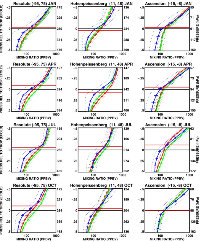
Fig. 11. Modeled and observed monthly average ozone profiles from the 2◦×2.5◦run at the stations of Resolute, Hohenpeissenberg, and

Ascension for the months of January, April, July, and October. Blue line with crosses: observed RTT-averaged profile. Error bars indicate ±2 times standard error. Red line: Modeled RTT-averaged profile. Green line: Modeled RTT-averaged profile, plotted relative to the observed monthly median tropopause pressure, rather than relative to the model monthly median tropopause pressure. Dash-dot lines indicate ±2 times the standard error limits. Dotted lines indicate ±1σ standard deviations. Black and red horizontal lines indicate observed and model monthly median tropopause pressures, respectively.

and measured RTT-averaged profiles at the same fraction of the tropopause pressure. (For instance, when y=.25, the observed profiles and the model profile represented by the green line are both a factor of e0.25higher than their respec-tive tropopause pressures.) The figure also indicates standard errors and standard deviations for each of the profiles.

The RTT-averaged model profiles shown in Fig. 11 re-produce the characteristic shapes seen in the observations, but typically with weaker cross-tropopause gradients result-ing in model high biases in the UT and sometimes low bi-ases above the tropopause. Model profiles can reproduce the observations quite well, such as at Hohenpeissenberg in July, but often the upper tropopause high bias is substan-tial. It is interesting to note that normalizing the model pro-files to the observed rather than modeled monthly median tropopause tends to increase the upper-tropopause high bias when the model tropopause lies above (at a lower pressure, which is typical) the observed monthly median tropopause, and decrease it when the model tropopause is found be-low the observed tropopause. This effect is distinct from the RTT-averaging process itself. While it is obvious that RTT averaging produces comparisons that better characterize model/measurement differences across the tropopause than pressure averaging, it is not clear if it is better to compare model and observed RTT-averaged profiles at the same pres-sure or at the same fraction of their respective tropopause pressures.

The standard error of the profiles shown in Fig. 11 are small and indicate that the mean profiles are known pre-cisely enough that the differences between them are signifi-cant. The standard deviations of the profiles shown in Fig. 11 provide a comparison of observed and modeled variability of daily O3profiles, separated from tropopause height

variabil-ity due to RTT-averaging. Here we see that the model vari-ability is weaker than observed. This is not surprising. Nu-merous observations show that atmospheric O3has

substan-tial variability at scales much smaller than the model grid, which will be reflected in ozonesondes but not in model daily profiles.

Because model values in the profiles shown in Fig. 11 cor-respond to layer averages, there is a potential source of error in the comparisons because the RTT climatology was gener-ated by first interpolating daily ozonesondes to the RTT grid and then averaging the values. Thus, a value in an RTT pro-file does not represent a layer average if there is a nonlinear change in O3between the bottom and top of the layer. We

do not think this is a significant error. Because the effective vertical resolution of the sondes is about 300 m due to the time it takes to pump air through the sonde, there are typi-cally only 3–4 points per layer – a small number with which to resolve any nonlinearity. We also tested the differences between interpolated values and layer averages by generat-ing pseudo high-resolution profiles from the RTT climatol-ogy using cubic spline interpolation, and then constructing layer averages. This resulted in only ∼ 1–3% differences,

showing that our method of constructing the RTT climatol-ogy is not a problem.

Figure 12 shows percent differences between the model and observed monthly mean profiles for the three sta-tions shown in Fig. 11. (Note the larger vertical range in Fig. 12.) Here we show percent differences between model and observed pressure-averaged profiles (red), RTT-averaged profiles (blue), and RTT-RTT-averaged profiles normal-ized relative to the observed tropopause (green). Figure 12 shows better agreement between the modeled and observed pressure-averaged monthly mean ozone profiles than the RTT-averaged profiles, as expected. The pressure-averaged profiles show moderate model high-biases in the UT by ∼20– 50%. The bias in the lower stratosphere is smaller in mag-nitude and more variable between a high or low bias than in the UT. When RTT-averaging is used, biases between the model and the observations are larger; differences are typi-cally about ∼50%, but can exceed 100% (blue lines). When RTT-averaged profiles are compared at the same fractional value of the tropopause pressure (green lines), the model upper tropospheric high bias tends to be increased when the model tropopause pressure is lower than the observed tropopause pressure, as was also shown in Fig. 11.

Figure 13 is a bar chart summarizing April percent differ-ences between the 2◦×2.5◦ model run and observed ozone in the UT, at a pressure one quarter of an e-fold higher than the tropopause pressure. April is shown because the largest UT model discrepancies from observations occur in the March/April time period, while the smallest occur in June and July. Figure 13 illustrates that RTT-averaged (blue bars) and RTT-averaged profiles normalized to the observed tropopause (green bars) typically show substantially larger biases than the pressure-averaged profiles (red bars) at both the tropical and NH stations. The tropical stations of Para-maribo, Kuala Lumpur, San Cristobal, Nairobi, and Malindi exhibit particularly small biases. The mean NH pressure-averaged bias is ∼35%, which approximately doubles with RTT-averaging. In the tropical mean, there are ∼20% high biases in the pressure-averaged case vs. a ∼30% difference for RTT-averaged profiles, resulting in a ∼50% difference between the averaging techniques.

Figure 14 shows the biases at all stations in the lower stratosphere, at a pressure one quarter of an e-fold below the observed monthly median tropopause pressure. Agree-ment in the lower stratosphere is generally substantially bet-ter than in the upper troposphere, with mean biases in the NH and the tropics <20%. Here, the RTT-averaged and normal-ized RTT-averaged biases are typically more negative than the biases between pressure-averaged profiles. This is the expected behavior of a profile with a weak cross-tropopause gradient – high biases in the UT, and low biases in the lower stratosphere. The five tropical stations with small UT high biases are shown here to have more substantial low biases in the lower stratosphere, indicating that the agreement of model cross-tropopause gradients with observations at these

Resolute (-95, 75) JAN -100 -50 0 50 100 PERCENT DIFFERENCE -1 -.75 -.5 -.25 0 .25 .5 .75 1 PR ESS R EL T O T R O P (EF O L D ) 106 137 175 225 289 371 476 612 786 Hohenpeissenberg (11, 48) JAN -100 -50 0 50 100 PERCENT DIFFERENCE -1 -.75 -.5 -.25 0 .25 .5 .75 1 82 106 136 174 224 288 369 474 609 Ascension (-15, -8) JAN -100 -50 0 50 100 PERCENT DIFFERENCE -1 -.75 -.5 -.25 0 .25 .5 .75 1 33.5 43.0 55.2 70.9 91.0 116.8 150.0 192.6 247.4 PR ESSU R E (h Pa ) Resolute (-95, 75) APR -100 -50 0 50 100 PERCENT DIFFERENCE -1 -.75 -.5 -.25 0 .25 .5 .75 1 PR ESS R EL T O T R O P (EF O L D ) 119 153 197 252 324 416 534 686 881 Hohenpeissenberg (11, 48) APR -100 -50 0 50 100 PERCENT DIFFERENCE -1 -.75 -.5 -.25 0 .25 .5 .75 1 89 115 147 189 242 311 400 513 659 Ascension (-15, -8) APR -100 -50 0 50 100 PERCENT DIFFERENCE -1 -.75 -.5 -.25 0 .25 .5 .75 1 35 44 57 73 94 121 155 199 256 PR ESSU R E (h Pa ) Resolute (-95, 75) JUL -100 -50 0 50 100 PERCENT DIFFERENCE -1 -.75 -.5 -.25 0 .25 .5 .75 1 PR ESS R EL T O T R O P (EF O L D ) 96 124 159 204 262 336 432 555 712 Hohenpeissenberg (11, 48) JUL -100 -50 0 50 100 PERCENT DIFFERENCE -1 -.75 -.5 -.25 0 .25 .5 .75 1 79 101 129 166 214 274 352 452 580 Ascension (-15, -8) JUL -100 -50 0 50 100 PERCENT DIFFERENCE -1 -.75 -.5 -.25 0 .25 .5 .75 1 38 49 63 81 104 134 172 221 284 PR ESSU R E (h Pa ) Resolute (-95, 75) OCT -100 -50 0 50 100 PERCENT DIFFERENCE -1 -.75 -.5 -.25 0 .25 .5 .75 1 PR ESS R EL T O T R O P (EF O L D ) 104 134 172 221 284 365 468 601 772 Hohenpeissenberg (11, 48) OCT -100 -50 0 50 100 PERCENT DIFFERENCE -1 -.75 -.5 -.25 0 .25 .5 .75 1 75 96 124 159 204 262 336 432 555 Ascension (-15, -8) OCT -100 -50 0 50 100 PERCENT DIFFERENCE -1 -.75 -.5 -.25 0 .25 .5 .75 1 36 46 60 76 98 126 162 208 267 PR ESSU R E (h Pa )

Fig. 12. Percent difference of modeled from observed monthly mean ozone profiles at Resolute, Hohenpeissenberg, and Ascension for

the months of January, April, July, and October. Red lines: percent difference between pressure-averaged profiles. Blue lines: percent difference between RTT-averaged profiles. Green lines: percent difference between model and observed RTT profiles, with the model profile normalized to the observed tropopause pressure so that the difference is taken at the same relative fraction of the tropopause pressure. Dotted lines indicate ±2 times the standard error.