Non-linear and non-stationary hydroclimate variability in France and the Euro-Atlantic area

HAL Id: tel-02934594

https://tel.archives-ouvertes.fr/tel-02934594

Submitted on 9 Sep 2020

HAL is a multi-disciplinary open access archive for the deposit and dissemination of sci-entific research documents, whether they are pub-lished or not. The documents may come from teaching and research institutions in France or abroad, or from public or private research centers.

L’archive ouverte pluridisciplinaire HAL, est destinée au dépôt et à la diffusion de documents scientifiques de niveau recherche, publiés ou non, émanant des établissements d’enseignement et de recherche français ou étrangers, des laboratoires publics ou privés.

Non-linear and non-stationary hydroclimate variability

in France and the Euro-Atlantic area

Manuel Fossa

To cite this version:

Manuel Fossa. Non-linear and non-stationary hydroclimate variability in France and the Euro-Atlantic area. Earth Sciences. Normandie Université, 2020. English. �NNT : 2020NORMR011�. �tel-02934594�

THESE

Pour obtenir le diplôme de doctorat

Spécialité Sciences de l’Univers

Préparée au sein de l’Université de Rouen

Non-linear and non-stationary hydroclimate variability in France

and the Euro-Atlantic area

Présentée et soutenue par

Manuel FOSSA

Thèse dirigée par Nicolas MASSEI laboratoire UMR 6143 Morphodynamique Continentale et Côtière

Thèse soutenue publiquement le (date de soutenance) devant le jury composé de

David HANNAH Professor / GEES / University of Birmingham Rapporteur Benoit HINGRAY Chargé de Recherches HDR / IGE / Université de Grenoble Rapporteur Michael GHIL Distinguished Professor / TCL / University of California Rapporteur Laurie CAILLOUET Ingénieure / hydrométéorologue / Compagnie Nationale du Rhône Examinatrice Monica IONITA Research Scientist / Paleo-climate Dynamics / Alfred Wegener Institute Examinatrice Nicolas MASSEI Professeur / M2C/ Université de Rouen Normandie Directeur de Thèse Benoit LAIGNEL Professeur / M2C/ Université de Rouen Normandie Co-Directeur de Thèse Matthieu FOURNIER Maitre de conférences HDR / M2C / Université de Rouen Normandie Co-Encadrant de Thèse Claire MAGAND Chargée de Projet / Office Français pour la Biodiversité Membre Invitée Bastien Dieppois Assistant Professor / CAWR / University of Coventry Membre Invité

Cette thèse, réalisée au sein du laboratoire M2C de l’université de Rouen et en cofinancement avec l’Office Français pour la Biodiversité, a bénéficié du financement de la Région Normandie, avec l’appui de la fédération FR3130 SCALE.

Acknowledgements

この論文は、私の母、亡くなった父（毎日欠場する）、そして私の家族や大切な友人に捧げ られています。本当に旅行でした,この論文は. 最初は速く走りましたが、その後、落ちまし た. しかし、私の友人と家族はいつも私を助けてくれました. 彼の無限のサポートのために,最初 に Nicolas Massei に感謝したい. 彼はつらい時でもいつも私を支えてくれました. この男 はまだ私が見ているモデルであり、真の科学者です.Nicolas, ありがとう！ 私のもう一人の 友人、Bastien Dieppoisに感謝したい. 彼がいなければ、私はこの論文を完成させなかった だろう. 彼の上司は、私を助けてはいけないと言ったが、彼は私と一緒に一日中過ごした。 Bastien先輩, 心から感謝します！別の非常に重要な人物はKenneth Stephensonさんです. 彼 がいなければ、私はこのExtremal lengthに取り組むことができなかっただろう. これは私に 全く新しい世界を開いた. ありがとう,Stephensonさん! MatthieuとBenoitのサポートに感謝 します. Criannのすばらしいサービスに感謝します. Gill MorelとCharles Feibel、私の奇 妙な要求に我慢してくれてありがとう! クロススケール相互作用アルゴリズムで私をサポー トしてくれたNicola Jajcayにも感謝します. Claire Magand、私の遅れた仕事に我慢してくれてありがとう, ごめんなさい! M2Cは家族のようなものです。たくさんの素晴らしい友達に会いました！これらの絆は確か に私たちが苦難に耐えることを助けました, そして私たちのジョークは私たちの記憶に永遠 にとどまるでしょう. 私たちは悲しいことについても冗談を言うために使用します.例えば ,Jewとtata,BiatchとChoucroutyとAbdel, Flaviereの疲れる屋外キャンペーン. 良いことが たくさんありました: Lycaonsのお尻をなめるとか, 「Président Voleur!」の歌とか, 「Le masque de faire」についてのジョークとか,crossfit girlとMarthe,Clef à moletteと私の Fort de caféなContrition, 等々… たくさんの笑いがありました! だから, Jew,Biatch,Clef à Molette,Choucrouty,Louise,Flavière,Senpai,Doudou,Connasse,David,Ruth,Thomas,Antoni n,Valentin,Léo,Micheeeeeeeeeellllllll,Max,Yoann,Theo, M2Cの科学者、MoussMouss, Maria, Cécile…S また、STEその後ESEBのクラスメートにも感謝したいと思います, あなたは私を10歳若く感じ させました！だから, Doudou, Laurent, Mathije, Zou des bois, Natacha, Julie,

Marion, DoudouのMarion, Tite Aurore, Raph,…. Kathleen, Marie “wild” Lenoir, 47% (冗談!冗談よ! 愚痴の束! あなたを平手打ちしたかったねえ!)

みんな……

どうもありがとう!!

Table of contents

Avant-propos………..i

Table of contents………...vi

Introduction………...1

Part I – Spatiotemporal Scales of Hydroclimate Variability in France………...21

Part II – Spatiotemporal Scales of the Large-scale Hydroclimate Variability…49 Part III – Dynamics of the North Atlantic atmospheric circulation………77

Part IV – General Discussions & Conclusion………...115

References……….125

Supplementary material……….146

1. Background

France is one of the wealthiest countries in Europe and is water-independent as far as water access is concerned (Richard et al. 2010). However, there are topics, pertaining to water resources, which are of significant concern in France. Despite the large supply of water, shortage periods regularly occur during summer, especially in southern France, due to exceeding exploitation (Richard et al. 2010). A large part of this exploitation is tied to energy production and irrigation, fluctuating depending on the needs (Colon et al. 2018). Natural hazards represent another variable source of concern (Richard et al. 2010).For instance, France has experienced significant drought and flood episodes during the last 20 years. The 1999 windstorms and floods caused 140 deaths over France, southern Germany, Switzerland and Italy, while the 2003 heatwaves, accompanied by severe droughts, caused the deaths of 14802 people (Boccard 2018). In the above mentioned example, the natural variability of the hydroclimate system proved to be unpredictable, so that management policies could not anticipate the fore coming issues, which had severe consequences, both on people and economy. A complete understanding of hydroclimate variability is indeed challenging. The hydrosphere is an integral part of the climate system and is in constant interaction with the atmosphere, lithosphere, cryosphere and biosphere (Gettelman and Rood 2016). Figure I.1a-b illustrates the different components impacting hydrological system, as well as their spatial and temporal scales. Any change in one of the compartment may affect the others (Kingston et al. 2020).

Figure I.1. The spatial and time scales of the Hydroclimate system. a) The different

components of the hydroclimate system and their interactions; b) The spatial and temporal scales of hydroclimate variability. (IPCC 2007;Kingston et al. 2020)

a)

This results in high degrees of non-linearity, as well as non-stationarity, amplified by human activities, such as changes in land-use, demographic explosion, as well as rising temperature at the global scale in response to an increasing greenhouse release in the atmosphere (IPCC 2007). Even though an increasing number of studies focus on describing non-stationarity, very few link it to non-linearity, which leads to partial understanding of the complex hydroclimate dynamics (Blöschl et al. 2019). In addition, studies examining hydroclimate variability have been scarce in France, and often localized in time scale or space (Sauquet et al. 2008; Boé 2013; Boé and Habets 2014; Caillouet et al. 2016; Dieppois et al. 2016a). This leaves many questions as to how the non-linearity and non-stationarity shapes the temporal and spatial scales of hydrological variability (Blöschl et al. 2019).

2. Literature review

2.1. Hydrological variability in France

At the seasonal scale, discharge variability in France is spatially dependent on the rainfall and/or snowfall type defining the hydrological regime. North-western watersheds are driven by rainfall, with discharge peaking in winter while low discharge occurs in summer. Eastern and South-eastern watersheds are driven by snowfall (or by both rainfall and snowfall), with discharge peaking in spring (due to snow melt; Pardé 1933; Sauquet et al. 2008). Discharge in northern France have also been associated with significant annual, inter-annual (5-8 years’ time scales) and decadal variability (Massei et al. 2010; Fritier et al. 2012; Dieppois et al. 2016). Long-term variability, e.g. at decadal scales, in discharge have been shown to be a very important in trends detection over France. For instance, positive trends were initially found in northern France regions, i.e. in rainfall-driven regions, while negative trends were identified in the southern and eastern regions, i.e. regions where discharge is at least partially impacted by snowmelt (Stahl et al. 2010). However, using multi-temporal trend analysis, Hannaford et

variability. Accounting for decadal variability, Hannaford et al. (2013) identified positive trends in southern and eastern regions, while no significant trends were found in the northern regions.

The spatial homogeneity in discharge variability has been investigated at several time scales, on average, and in high- (flood) and low- (drought) flows. Results from previous studies vary greatly depending on the timescales. For instance, twelve regions were found by Sauquet et al. (2008) for monthly runoff, while, at decadal timescales, Hannaford et al. (2013) found five regions across Europe, where the stations in France represented only one region (Central west). According to Gudmundsson et al. (2011a), high, mean and low discharge also influences the spatial coherence. For instance, at spatial scales lower than 400 km, high-flows were found to be more homogeneous spatially than mean- and low-flows (Gudmundsson et al. 2011a). Reversely, when considering larger spatial scales, greater than 800 kilometres, low flows regions tend to become more homogeneously spatially distributed (Gudmundsson et al. 2011a). The possible reason behind this distinction is the different processes associated with high- and low-flows (Gudmundsson et al. 2011a): high-flow being tied to water input, while low-flows is tied to depletion of storage. Thus, focusing on flood event distribution, Mediero et al. (2015) found five homogenous regions across Europe, with France being characterized by three regions.

2.2 Drivers of discharge variability in France

Discharge is primarily impacted both by watershed characteristics, precipitation and evapotranspiration (mostly driven by temperature; Gudmundsson et al. 2011). While rainfall originated from large-scale climate/weather system beyond the catchment scale, effective precipitation, i.e. precipitation minus evapotranspiration, is then modulated by watershed characteristics, hence creating a complex, feedback driven, climate-to-discharge system (Boé 2013).

2.2.1 Watershed characteristics

Morphology of the catchment, soil types, evapotranspiration, land-use and groundwater support are examples of watershed characteristics, commonly associated with driving discharge variability. Three types of ground water support, with decreasing transfer types, are found in France, respectively named as: matrix, fractured matrix, and karstic. Depending on the location, either or both three types can be found, and this is deeply affecting how the precipitation input is transferred to discharge via groundwater support. For instance, in the Seine river watershed (northern France), karstic network communication with the fractured matrix have been shown to induce two flow regimes one as a conduit, and other as a storage, while their behavior was being controlled by the hydraulic gradient inside the matrix (El Janyani et al. 2012). According to Labat et al. (2000), the dynamics of the watershed groundwater support is thus catchment specific, non-linear and non-stationary. Such watershed properties were taken into account in previous classification of discharge variability in France by Sauquet et al. (2008). Through complex processes of surface saturation, soil properties variability also impacts the discharge variability in a non-linear way. This was, for instance, demonstrated in regions vulnerable to flash floods, where soil properties control the discharge until surface saturation occurs, after which rainfall becomes the primary driver (Anquetin et al. 2010).

2.2.2 Precipitation-watershed characteristics feedback

Soil moisture in France has been found to have significant impact on local precipitation (Boé 2013; Laaha et al. 2017). However, such feedback depends on the related large-scale climate pattern. As illustrated in Boé (2013), a negative feedback was observed during a negative North Atlantic Oscillation (NAO), while a positive feedback was observed during Atlantic Low conditions. With a higher- than-global temperature increase over France for the last 40

years, the relationship between precipitation, soil moisture and evapotranspiration is thus becoming crucial (OECD 2013).

Figure I.2. Position of the polar and subtropical jet streams. The high altitude jets blow

eastward and delimit the zone (orange) of westerlies. (Taken from www.3bmeteo.com/). 2.2.3 Large-scale climate

The large-scale atmospheric circulation, modulating precipitation and temperature, can be investigated through atmospheric pressure patterns. Under the geostrophic approximation, winds indeed flow parallel to isobar lines, with increasing velocity proportional to the gradient between isobar lines.

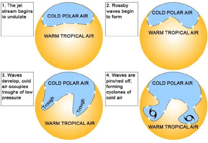
Figure I.3. Formation of the Rossby waves inside the polar jet stream. 1) The jet stream

forms around the zone of maximum pressure gradient between the cold polar air, and the warm tropical air. As warm air is less dense than cold air at the same atmospheric pressure, temperature differences starts to form along isobaric lines, i.e. baroclinic situations develops, triggering deviation of the jet from a pure zonal motion. 2) Because the absolute vorticity is conserved, any poleward motion of the jet increases the planetary vorticity, while the relative vorticity decreases, yielding a southward motion. When the jet has reached a certain equatorward position, the situation reverses, relative vorticity increases, planetary vorticity decreases, and the jet has now a northward direction. This process is then repeated, yielding the Rossby waves. 3) Because of the alternate northward and southward motions, troughs become associated with cyclonic conditions, and ridges with anticyclonic conditions. 4) At one point, the wave structure breaks and some troughs get disconnected from the wave train, becoming storms. Source: www.abc.net.au

2.2.3.1 North Atlantic atmospheric circulation

The North Atlantic is a major source of precipitation and temperature variability, due to the strong westerlies, carrying moisture and heat towards Europe (Ghil and Lucarini 2019).Those westerlies flowing from the high altitude at high speed are associated with the mid-latitude jet streams, mainly (Figure I.2). There is however another jet in the subtropical regions (Figure I.2), which is particularly important for the Mediterranean regions (Lionello et al. 2006). Both jets are due to the Coriolis force. The equator-pole differential heating induces an advection of heat from the equator to the poles, however, due to the Coriolis force (also called the planetary vorticity), this advection is progressively deviated clockwise in the Northern Hemisphere, yielding eastward winds.

The mid-latitude jet, which affects Europe climate the most (Ghil and Lucarini 2019) , arises from the high pressure gradient between the cold air from the pole encountering warm air coming from the equator (Ghil and Lucarini 2019), It has a wave-like structure in response to the strong zonal temperature gradients, which prompts deviation from a pure zonal advection (in addition to orography effects in some regions; Ghil and Lucarini 2019). As the absolute vorticity is preserved, there is a balance between the relative and planetary vorticities, leading to a wave-like pattern. These waves developing inside the jet stream are called Rossby waves (Figure I.3; Ghil and Lucarini 2019). Those waves propagate eastward with the jet stream, but may become stationary or stalled, yielding persistent weather conditions in regions below ridges or troughs (Ghil and Lucarini 2019; Mann 2019). Troughs of the Rossby wave eventually lump apart forming storms, that progress eastward too (Ghil and Lucarini 2019).

2.2.3.2 Weather patterns

Depending on the shape of the mid-latitude jet stream, i.e. the development and evolution of Rossby wave trains, three types of North Atlantic atmospheric patterns are commonly found

(Mo and Ghil 1987) zonal, blocking and wave train. Zonal patterns involve isobaric lines being orientated East/West leading to westerlies following a straight-line (Figure I.2). Blocking patterns are associated with a high pressure system blocking the jet stream, forcing it to deviate, forming a ridge and inducing dry conditions south of the ridge (Figure I.5). Wave train patterns are associated with successions of troughs and ridges, forming meridional winds (i.e. winds with significant poleward components), and yielding to persistent dry/wet weather when this system is stable, or to fast changing weather if the wave train is not stabled (Petoukhov et al. 2013). Depending on the time scales, those patterns may be observed directly (short term), or as anomalies (longer term; Cassou 2004; Hauser et al. 2015).

The NAO, and its positive and negative phases, have been observed since the early 20th century (Figure I.4a-b, I.5; Visbeck et al. 2001; Cassou et al. 2004; Hurrell and Deser 2014). The positive phase of the NAO triggers a zonal atmospheric circulation (Figure I.5). The negative phase however creates a blocking situation, responsible for the difference in weather found in France (Figure I.4). The dipole structure is not zonally symmetric, in the positive phase, the dipole is titled toward the East, and reversely for the negative phase (Figure I.4a-b; Visbeck et al. 2001; Cassou et al. 2004; Hurrell and Deser 2014).

Figure I.4. Statistical weather patterns: a-d) Pressure anomalies (in mgp) contours,

isolines and frequency of occurrence (in %) associated with each statistical weather patterns; e-h) the number of days of occurrence per year (histogram) of each statistical weather patterns, compared to the NAO index (top panels, orange curves).(Cassou 2010)

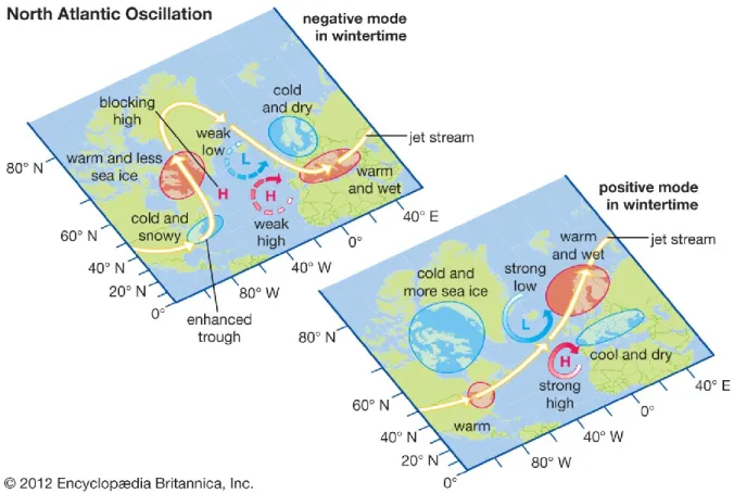
Figure I.5. Positive and negative phases of the North Atlantic Oscillation Encyclopaedia Britannica (2012). The structure of the North Atlantic Oscillation is the Icelandic low and

the Azores high dipole. In the positive phase (lower map), the Icelandic low is strong (i.e. very low pressure), while the Azores high is strong as well (i.e. very high pressure), the jet stream is channeled in between the dipole, resulting in warm and wet winters in Northern Europe, and cool and dry winters in Southern Europe. In the negative phase, the Icelandic low and Azores high are weak, so that overall the dipole disappears, creating a blocking condition in Mid North-Atlantic. The jet stream has to go around that blocking, triggering Rossby waves, and advection of warm air on the American side, and advection of cold air on the European side. In Northern Europe, the winters are cold and dry, in Southern Europe, they are warm and wet

2002; Folland and Knight 2009; Bladé et al. 2011; Giuntoli et al. 2013). The relationship between the NAO and hydroclimate over France has been found at multiple timescale from seasonal to multi-decadal time scales (Fritier et al. 2012; Massei and Fournier 2012; Boé 2013; Boé and Habets 2014; Ullmann et al. 2014; Hermida et al. 2015; Dieppois et al. 2016a). This relationship also appears to be modulated by soil moisture (Bladé et al. 2012). The positive phase of the NAO has been dominant from the 1960s to the mid-1990s (Figure I.4f), and has been associated with higher than normal streamflow anomalies (Massei et al. 2010). It has also been to a North-eastward shift in storm tracks near Iceland and the Norwegian Sea (Hurrell and Van Loon 1997), and an increase of river flow in the North, and a decrease in the South of Europe (Shorthouse and Arnell 1997; Ullmann et al. 2014). We also note that the decadal and multi-decadal NAO variability has been increasing since the mid-19th century (Goodkin et al. 2008; Sun et al. 2015) with an associated increased variability of precipitation and streamflow over France (Dieppois et al. 2016a).

The relationship between NAO and hydroclimate depends greatly on the region and the time scale. For instance, even in Northern France, where significant links were found at decadal time scales (Massei and Fournier 2012), the links between hydroclimate variability and NAO, depends on the location (Dieppois et al. 2013). In the Mediterranean, clear links between hydroclimate and the NAO occur at the quasi-decadal time scales (Feliks et al. 2010), but at the monthly time scales, different rainfall patterns are linked to either phase of the NAO, or other weather patterns (Ullmann et al. 2014).

In addition to the NAO, two blocking patterns are also frequently associated with weather in Europe (Cassou 2004). The Atlantic ridge (AR) is characterized by a high pressure system over North Atlantic, just south of Greenland (Figure I.4c). AR patterns are associated with cold, but rainier weather over France, especially in the North (Boé 2013). Since 2001, there

compared to the NAO regimes (Hurrell and Deser 2009; Hauser et al. 2015; Hanna et al. 2016). The Scandinavian blocking (SBL) is a large high pressure centre over Scandinavia (Figure I.4d), which brings cold air over Central Europe, and can potentially migrates westward towards France (Cassou 2010; van der Wiel et al. 2019).

2.2.4 Ocean-hydroclimate variability interactions

The North Atlantic atmospheric circulation variability has been shown to significantly interact with North Atlantic sea surface temperature (SST) from monthly to multi-decadal time scales. At monthly timescale, the preferred direction of the interactions is from the atmosphere to the SST. A positive NAO is followed by positive SST anomalies in the western subtropical North Atlantic and negative SST anomalies in the subpolar gyre and off the eastern coast of North Africa, referred to as the SST ‘‘tripole’’, and reversely during a negative NAO (Kushnir et al. 2002)However, In early winter, the NAO also responds to slightly different tripolar SST anomalies, amplifying the NAO and acting as a positive feedback (Czaja and Frankignoul 1999, 2002; Gastineau and Frankignoul 2014). Whether such active ocean–atmosphere coupling has a significant influence on decadal climate variability has been mostly investigated using climate models. Two-way ocean–atmosphere interactions in the North Atlantic can be the dominant players, as suggested in Timmermann et al. (1998). In winter, Gastineau and Frankignoul 2012 showed that AMOC intensification and the associated subpolar warming lead to a negative NAO in winter in six climate models. Meanwhile, a gulf stream like SST front keeps the jet stream stationary, and modifies its shape at different pressure levels (Feliks et al. 2016). In summer, the largest atmospheric response to SST resembles the EA pattern and results from a combination of subpolar and tropical forcing (Gastineau and Frankignoul 2014).

At decadal to multi-decadal time scales, the North SST variability is dominated by the Atlantic Multi-decadal Oscillation (AMO; Gastineau and Frankignoul 2014), which has been found to be linked to the AMOC (Gastineau and Frankignoul 2014). A warm AMO leads to atmospheric warming in summer, but a negative NAO in winter (Gastineau and Frankignoul 2014).

The impact of the SST variability on rainfall and river flows has received significant attention, especially for decadal time scales and higher. For instance, the AMO has been found linked to changes in the frequency of occurrence of extremes events in both North America and western Europe (Sutton and Hodson 2005; Sutton and Dong 2012). In particular, a shift in the AMO during the 1960s may have resulted in a cooler US and European climate, before another shift led to a warming phase (Sutton and Hodson 2005; Sutton and Dong 2012). The relationship between SST and extreme events is not limited to the North Atlantic, as evidence shows that the Mediterranean basin experiences the same type of relationships, a warmer (cooler) Mediterranean Sea leading to changes in the rainfall weather patterns over the Mediterranean regions (Polo and Schiemann 2013). The relationship between AMO and rainfall in northern France has only been observed at the 30-60yr’ time scales, while the relationship between AMO and temperature has been observed at all inter-decadal to multi-decadal time scales (i.e. 16 year to 80 year' time scales; Dieppois et al. 2013b). The relationship between SST and temperature has been established for the European drought in 2015, with negative SST anomalies in the central North Atlantic ocean, and positive ones in the Mediterranean (Ionita et al. 2017).

2.2.5 Atmospheric circulation dynamics

The atmospheric circulation variability, i.e. the trajectory in the system’s phase space, displays multiple equilibria, i.e. stationary states, identified physically at monthly time scales,

and statistically at annual time scales, as zonal and blocking patterns (Hauser et al. 2015; Ghil et al. 2018). While the zonal states are identified with the eastward mid-latitude jet stream circulation, the blocking patterns have been tied to slowly moving Rossby waves, although the controlling factors of their persistence is still up to debate (Ghil et al. 2018). According to Ghil et al. (2018, and references therein), Stephenson et al. (2004) explains the slow moving Rossby waves by the interference between slowing Rossby waves, while Hannachi et al. (2017) evokes the creation of topographic Rossby waves of different wavenumber that enter in resonance. An alternative view, is that of energy leaks through a waveguide’s boundaries, associated with resonant dynamics, the so called “quasi-resonant amplification” (Mann et al. 2018). This difficulty in understanding the cause of persistent blocking patterns lies in the fact that the mechanisms governing the dynamics of Rossby waves, especially the nature of the restoring force, are still under debate (Cai and Huang 2013). The dynamics about those equilibria are also complex, with known bifurcations, stable and unstable transitions (Michael Ghil and Childress 1987). The approaches about those transitions are either considered non-linear deterministic or non-linear stochastic (Ghil 2019; Ghil and Lucarini 2019).

The combination of atmospheric models, coupled with topography has allowed to describe, at least at the daily to monthly time scales, that zonal patterns had two-way transitions from/to wave train patterns, and one-way transitions to blocking patterns (Michael Ghil and Childress 1987). Using more realistic topography, the NAO and Atlantic Oscillation phases were found as stationary states, with direct transitions from each other states possible, except from AO+ to AO- and reversely (Kondrashov et al. 2004). At inter-annual scales, only statistical work has been done. The NAO and scandinavian blocking-like phases have been found as stationary states (Hauser et al. 2015). Yet their transitions were only established along a time series, and not from a phase space point of view (Hauser et al. 2015).

3. Research objectives and methods

This thesis aims at better understanding the non-linearity and non-stationarity of hydroclimate variability. Particularly, we aim at studying how the complex interactions between hydrological, local and large-scale climate variables shape the spatiotemporal hydroclimate variability in France.

The main research objectives of this thesis are as follows:

 Determine regions of homogeneous hydroclimate variability in France, based on non-stationary spectral characteristics;

 Study non-linear interactions between the different timescales of hydroclimate variability to unravel their possible causal relationships;

 Study the non-stationary spectral characteristics of the watershed modulation of the local climate input;

 Discover non-linear, non-stationary, statistical and spectral spatiotemporal links between local and large-scale hydroclimate variables;

 Unravel stationary, stable or unstable states of the atmospheric circulation as well as their transitions.

Figure I.6 displays the datasets and methods used throughout this dissertation. The emphasis is given to methods allowing accounting for interactions between components of the hydroclimate system linearity), and abrupt changes in the dynamics of the system (non-stationarity).

Figure I.6. Datasets and methods used for this thesis. Red dots show gauging stations. The

total atmospheric spatial extent is called the Euro-Atlantic area.

4. Thesis outline

The Introduction provided a general introduction and a review of the current understanding of hydroclimate variability in France. In Part I, hydroclimate regions in France of homogeneous spectral variability are computed, then, interaction between their characteristic time scales are investigated. In Part II, spectral characteristics of both discharge and local climate variables (i.e. precipitation and temperature) are studied to identify potential modulations by the watershed properties on the climate input. Then, spectral characteristics of large-scale climate over the Euro-Atlantic area are compared to those of discharge. In Part

variability using the geometrics-physics correspondence, enabling to decouple the classical vision that associate one pattern with one and only one type of dynamics. Finally, the significance of these findings, their limitations and potential areas of further developments are discussed in the Conclusion.

P

ART

I:

S

PATIOTEMPORAL

S

CALES OF

H

YDROCLIMATE

Introduction

Hydroclimate variability represents the spatiotemporal evolution of climate variables (e.g. precipitation and temperature), which are directly impacting hydrological variability (e.g. streamflow, groundwater). Studying how hydrological variables react to climate variability and changes is a major challenge for society, in particular for water resource management and flood and drought mitigation planning (IPCC 2007, 2014).

Hydrological variability fluctuates at multiple timescales (Labat 2006; Schaefli et al. 2007; Massei et al. 2017), which are still poorly characterised and understood in term of driving-mechanisms. As suggested in Blöschl et al., (2019), understanding the spatiotemporal scaling,

i.e. how the general dynamics driving hydrological variability change at spatial and temporal

scales, represent a major challenge (Gentine et al. 2012). The objective is to identify critical scales, i.e. the maximum spatiotemporal scale at which the dynamics remain unchanged, also commonly called scaling invariance (Hubert 2001). Critical scales are characteristic of non-linear systems (Hubert 2001). In non-non-linear system, a slight change in a system parameters can results in large changes in the observed dynamics, as a result of complex interactions between system components, as demonstrated by Lorenz (1963).

Hydrological variability is by definition non-linear (Labat 2000; Lavers et al. 2010; McGregor 2017), as it results from complex interactions between atmospheric dynamics and catchment properties (e.g. soil, water table, karstic systems, vegetation; Gudmundsson et al., 2011; Sidibe et al., 2019). However, very little work has hitherto been done to understand how the different drivers of hydrological systems vary at multiple temporal and spatial scales. As suggested in Anishchenko et al. (2014), nonlinearity in physical processes is even more likely when time or spatial distance increases. This results in difficulties characterizing the hydrological variability at different spatiotemporal scales (Gentine et al. 2012; Blöschl et al.

transfer of dynamics from small to large scales, and closure, i.e. the different couplings between components of a system, as the most important challenges in modelling hydrological variability. However, while different time scales have been identified in hydrological variability at both global and regional scales (Coulibaly and Burn, 2004; Labat, 2006; Dieppois et al. 2016; Massei et al., 2017), very little has been done to explore how coherent are those time scales in space, and therefore in identifying critical scales in which all ranges of variability remain unchanged.

Studying 231 steam gauges throughout the world, Labat (2006) highlighted different time scales of streamflow variability over the different continents. At the regional scale, Smith et al. (1998) established a clustering of 91 US stream gauges based on their global wavelet spectra, i.e. dominant time scales, and found five homogeneous regions. Similarly, Anctil & Coulibaly (2004), and Coulibaly & Burn (2004) for Canada, established a clustering of southern Québec streamflow, based on the timing of both the 2-3 and 3-6 year time scales, distinguishing the northern and southern regions. In Europe, Gudmundsson et al. (2011) identified different regions according to their low-frequency fluctuations (defined by the authors as timescale of variability greater than 10 years). In France, such clustering based time-frequency patterns of streamflow variability, as well as its relation to climate variability (e.g. precipitation and temperature), has not yet been explored. In addition, all the studies mentioned above either isolate different time scales or average the variability across time scales (e.g. global wavelet spectra), which is equivalent to a linearization of the system (Hubert et al., 1989). In this study, we propose to combine wavelet analysis and a new fuzzy-clustering algorithm to understand the spatial coherence of precipitation, temperature and streamflow variability over France in fully non-linear approach accounting for both time and frequency domains.

The work is divided into the following parts. Data and methods are introduced in Section 1. In Section 2, we cluster precipitation, temperature and discharge variability based on their scale-time patterns. Couplings between the different scale-time scales of variability are then explored in Section 3. Finally conclusion and discussion of the main results are provided in Section 4.

a) b)

Figure 1.1. Research area. a) Location of stream gauges (red dots) and their respective

hydrographic networks (blue lines); b) Orography over France, and delineation of mountain ranges.

1. Data and Methods

1.1 Hydrological and Climate Data

Discharge time series were extracted from the observation dataset introduced by Bourgin et

al. (2010a, b). This data set is composed of 4496 watersheds, their main river daily time series

and their hydrologic descriptions. This data set was initially subset to low anthropogenic influenced and low groundwater support watershed, comprising 662 stations. We further

reduced the data to 152 stream gauges, by keeping only continuous time series from January 1968 to December 2008 (Figure 1.1).

Figure 1.2. Workflow of this study. a.) 152 monthly precipitation, temperature and

discharge time series are extracted from IRSTEA’s watershed database. The following steps are applied to each variable; b.) The continuous wavelet spectrum for each watershed is computed; c.) A distance matrix between wavelet spectra is then established; d.) A fuzzy clustering algorithm is used to build a classification map of the watersheds based on their wavelet spectra.

Precipitation and temperature data have been estimated from the SAFRAN reanalysis data set (''Systeme d'Analyses Fournissant des Renseignements Adaptes a la Nivologie''; Vidal et al. 2010). The data is formatted as a regular rectangular grid of 8 kilometers’ spaced nodes that

covers metropolitan France. Data start in August 1958, and are regularly updated. For this study, the precipitation and temperature have been averaged over each watershed.

1.2 Methods

Figure 1.2 sums up the different steps of this study. First we compute the non-stationary spectral characteristics of each watershed precipitation, temperature and discharge, using continuous wavelet transforms (Figure 1.2, (a)). Then we use cluster the wavelet transforms of each watershed’s variable, using IEDC and fuzzy clustering techniques, which gives the spatial critical scales of homogeneous variability (Figure 2, (b)). We finally study the non-linear interactions taking place between the different time scales of each homogeneous region (Figure 1.2, (c)).

1.2.1 Continuous wavelet transforms

Scale-Time patterns have first been extracted for each watershed, and each variable, using continuous wavelet transform (cf. Figure 1.2, (a)). For any finite energy signal 𝑥, it is possible to obtain a scale-time representation by mapping it to a series of subspaces spawned by a generating function, the mother wavelet, and its scaled versions (Torrence and Compo 1998; Grinsted et al. 2004). The time series is then represented in terms of a given scale and time location. The first subspace is generated by a mother wavelet at scale 1 and its time translations. Then, other subspaces are generated by scaling the mother wavelet up, referring to daughter wavelets, and time translating it. For each scale, one subspace is constructed. Daughter wavelets are usually calculated as:

𝜓𝑎,𝑏 =

1 √𝑎𝜓 (

𝑡 − 𝑏

𝑎 ) (1)

The left hand side (LHS) term is the daughter wavelet of scale 𝑎 and time translation 𝑏 at time 𝑡. The first right hand side (RHS) term is the scaling of the mother wavelet 𝜓 and the last one is the time translation.

The projection of the signal onto each scale 𝑎 subspace is of the form: 𝑊𝑇_𝜓{𝑥}(𝑎, 𝑏) = < 𝑥. 𝜓_𝑎,𝑏 > = ∫ 𝑥(𝑡)𝜓_𝑎,𝑏(𝑡)𝑑𝑡

𝑅 (2)

LHS term contains the wavelet coefficients, i.e. the coordinates of the signal in each subspace. If the mother wavelet (and hence the daughter wavelets as well) is complex, wavelet coefficient are complex as well. Wavelet coefficients represent the inner product of the signal and daughter wavelet of scale 𝑎 and time translation 𝑏 (Centre Hand Side). The norm of their square is called the wavelet power and represents the amplitude of the oscillation of signal 𝑥 at scale 𝑎 and centred on time 𝑡. As it is impossible to capture the best resolution in both and time at the same time, here, we used a Morlet mother wavelet (order 6), which offers a good compromise between detection of scales and localisation of the oscillations in time (Torrence and Compo 1998).

1.2.2 Image Euclidean Distance Clustering

As shown in Figure 1.2(b), the similarities between wavelet spectra of each watershed, and, separately, on each variable, have been estimated. Distances between 2-dimensional data, such as maps or wavelet spectra, are commonly estimated using Euclidean distance between pairwise points (pED; i.e computing 𝑓2(𝑥1, 𝑦1) − 𝑓1(𝑥1, 𝑦1)). However, such a procedure has

no neighborhood notion, making it impossible to account for globally similar shapes (cf. definition of global and local similarity in Wang et al. 2005).

To avoid this issue, Wang et al. (2005) developed the Image Euclidean distance calculation method (hereinafter IEDC). The IEDC method modifies the pED equation in two ways (Wang et al. 2005): i) the distance between pixels values is computed not only pairwise, but for all indices; ii) a Gaussian filter, function of the spatial distance between pixels, is applied. The Gaussian filter then applies less weight to the computed distance between very close and far apart pixels, while emphasizing on medium spaced ones (Wang et al. 2005).

1.2.3 Fuzzy clustering

Fuzzy clustering has then been used to cluster the different watershed based on their similarities (Figure 1.2, (b)). Fuzzy clustering is a soft clustering method (Dunn 1973). While soft clustering spreads membership over all clusters but with varying probability, hard clustering attributes each station one and only one cluster membership. Soft clustering is therefore better-suited when the spatial variability, originating from different stations’ characteristics, is smooth, such as in hydroclimatic data.

For instance, precipitation and temperature patterns are unlikely to change suddenly from one station to a neighboring one, and in turn, markedly different from the next neighbor (Moron et

al., 2007; Lloyd-Hughes et al., 2009; Rahiz & New, 2012). As such, several stations tend to

show transitional or hybrid patterns, and can potentially be member of different clusters, limiting the robustness of hard clustering procedure (Liu and Graham 2018). In this study, we used the FANNY algorithm (Kaufman & Rousseeuw, 1990). Fuzzy clustering performance is determined by the ability of the algorithms to recognize hybrid stations (i.e. stations incorporating multiple features from different patterns observed in other coherent regions), while allowing for a clear determination of the membership of stations with unique features

modification of its exponent 𝑟, offering the possibility to adapt the clustering to the data, and to enhance performance (Liu and Graham 2018). A critical part is however the selection of the optimal number of clusters. Rather than setting the number arbitrarily, we use an estimation of the optimum number of clusters by first computing a hard clustering method: the consensus clustering (Monti et al. 2003). Thus, the number of clusters providing the best stability (i.e. the minimal changes of membership when new individuals are added) is considered optimal as recommended in Şenbabaoǧlu et al. (2014). The different clusters’ memberships are then mapped to discuss the spatial coherency of each hydroclimate variable (cf. Figure 1.2).

1.2.4 Cross scales interactions

For each variable and each cluster, cross-scale interactions have also been explored (Figure 1.2, (c)). Cross-scale interactions refer to phase-phase and phase-amplitude couplings between time scales of a given time series (Paluš, 2014; hereinafter PS14). Here, coupling means that the state (either phase or amplitude) of a signal 𝑦 is dependent on the state of a signal 𝑥. Such couplings are non-linear, and, therefore, if the amplitude of 𝑦 varies with the phase of 𝑥, the reverse is not necessarily true. Thus, in the classical setting, for any directional coupling (e.g. 𝑥 → 𝑦), there must be a lag in the relationship between 𝑥 and 𝑦 . When both oscillations are synchronized, changes in 𝑥 affect 𝑦 in the same way changes in 𝑦 affect 𝑥, and a symmetry takes place. In that case, the 𝑥 → 𝑦 relationship may either have a lag shorter than the time series time step or be part of a larger system (Pikovsky et al., 2001). The different couplings describe causality relationship, such as described in (Granger 1969), referring to information transfer from one part of the signal to another. Granger causality is the potential for improving the prediction of the future of 𝑦 knowing information about the past of 𝑥. Following PS14 and Jajcay et al. (2018), who compares the most used methods when

studying causality, we choose the conditional mutual information (CMI) surrogates method, combined with wavelet transforms.

First, using a Morlet mother wavelet, the instantaneous phase and amplitude at time 𝑡 and scale 𝑠 of the signal are obtained. Next, the conditional mutual information, 𝐼(𝜙𝑥(𝑡); 𝜙𝑦(𝑡 +

𝜏) − 𝜙_𝑦(𝑡)|𝜙𝑦(𝑡)) for the phase and 𝐼(𝜙𝑥(𝑡); 𝐴𝑦(𝑡 + 𝜏)|𝐴𝑦(𝑡)), 𝐴𝑦(𝑡 − 𝜂)), 𝐴𝑦(𝑡 − 2𝜂)) for

amplitude is computed. In the case of the phase-phase, the CMI measures how much the present phase of 𝑥 contains information about the future phase of 𝑦 knowing the present value of 𝑦. For the amplitude, CMI measures how much the present phase of 𝑥 contains information of the future amplitude of 𝑦 knowing the present and past values of 𝑦. The statistical significance of the CMI measure is assessed using 5000 phase-randomized surrogates, having the same Fourier spectrum, mean and standard deviation as the original time series, as in Ebisuzaki (1997).

2. Spatiotemporal clustering of hydrological variability

The wavelet transforms of each station have been computed and checked for similarities using IEDC fuzzy clustering to identify homogeneous regions and characterize critical scales of hydroclimate variability over France. Cross scale couplings were then investigated for each homogeneous region.

2.1. Precipitation

2.1.1. Scale-time patterns

Seven regions with homogeneous scale-time patterns are identified (Figure 1.3a): North-western (#CL1-Pr, green), North-eastern (#CL2-Pr, blue), Centre-north (#CL3-Pr, red), Centre-western (#CL4-Pr, pink), Centre-eastern (#CL5-Pr, black), South-western (#CL6-Pr,

yellow) and South-eastern (#CL7-Pr, dark green). According to the global wavelet spectra (Figure 1.3b), precipitation is fluctuating at different time scales, ranging from seasonal to inter-annual (i.e. 2-8 years). The wavelet spectra (Figure 1.3c) show that those different time scales are non-stationary, with temporal changes in terms of amplitude discriminating the regions.

Figure 1.3. Clustering of precipitation scale-time variability in France. a.)

Classification map of the watersheds. Pie charts slices show the three highest probability a)

b)

memberships; b.) Global wavelet spectra for each cluster; c.) Statistically significant wavelet spectra for each cluster.

For instance, while other watersheds show sparsely significant annual variability, south-western watersheds are characterized by quasi-continuous annual variability until the late 1980s (Figure 1.3c). Similarly, although there is significant inter-annual variability in all watersheds from the late 1980s on the monthly wavelet spectrum, there is no significant inter-annual variability over the south-western and south-eastern watersheds (Figure 1.3c). Focusing on inter-annual time scales, however, significant fluctuations at ~4 and 8 years appear for those watersheds, yet, over shorter periods of time (Figure 1.4a-b).

In summary, different regions, coherent in precipitation variability, have been identified, and describe critical scales. The critical scales of homogeneous precipitation variability are significantly different depending on the region, for instance, Centre-eastern region (#CL4-Pr, black) covers 134km², while the Centre-western region covers more than 29000km² (Figure 1.1a). Interestingly, most regions seem delineated by orography (cf. Figure 1.1b), except for north-western watersheds.

2.1.2. Cross-scale interactions

Figure 1.5 shows cross-scale interactions for each cluster of precipitation variability identified in section 2.1.1.

As described in Figure 1.5a, north-western watersheds display bi-directional (i.e. feedback) phase-phase causality between 5-6yr and 6-7yr time scales variability. This suggests different physical processes at play within the 5-8yr variability, as displayed in Figure1. 3-4b. North-eastern watersheds display phase-phase causality from 4-7.5yr to 2-4yr time scales, as well as 3-5yr to 7-8yr time scales (Figure 1.5a). This suggests that the scale extent of the significant

Figure 1.4. Inter-annual precipitation scale-time variability in France. a.) Global wavelet

spectra for each cluster; b.) Statistically significant wavelet spectra for each cluster.

dynamics. Centre-northern watersheds show phase-phase causality from 2-3 to 3-4yr time scales, explaining the 2-4yr patch in Figure 1.3b. Two additional interactions take place, first from 6-7yr to 4.5-5yr, and from 7-8yr to 5.5-6yr time scales (Figure 1.5a), resulting in the 4-8yr inter-annual patch displayed in Figure 1.4b. Centre-eastern watersheds show phase-phase causality from 4yr to 6.5yr and from 7.5-8yr to 6.5-7yr time scales, resulting in the scale

a)

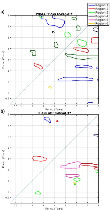
Figure 1.5. Precipitation cross-scale interactions. The driving scale is on the horizontal

axis, the driven on the vertical axis. a.) Phase-phase causality; b.) Phase-amplitude causality.

extent of the inter-annual patch in Figure 1.4b. South-western watersheds display phase-phase causality from 3.5yr to 1.5yr time scales (Figure 1.5a). Cascade phase-phase causality, i.e. sequential driving/driven relationships from higher (lower) to lower (higher) time scales, are observed in South-eastern watersheds. The phase-phase causality appears from 5-8yr to 4-5yr time scales over the same region (Figure 1.5a). Meanwhile, there is no phase-phase coupling

a)

Looking at phase-amplitude causality, north-western watersheds display interactions from 2-3yr to 1yr, from 6yr to 2yr, and from 8yr to 2-3yr time scales (Figure 1.5b). Thus, over this region, there is a link between higher time scales’ phases and lower time scales’ amplitude, resulting in significant patches in Figures 1.3b, 4a. North-western watersheds show phase-amplitude causality from 3-4yr to 7-8yr timescales (Figure 1.5b). Centre-northern watersheds display phase-amplitude causality from 2-3yr to 4yr, from 6-8yr to 3-5yr, and from 4yr to 7.5yr time scales (Figure 1.5b). South-western watersheds show isolated phase-amplitude causality from 6yr to 2yr time scales (Figure 1.5b). Centre-eastern watersheds show phase-amplitude causality from 8yr to 6yr time scales (Figure 1.5b). Centre-western regions show amplitude causality from 5-6 to 2-4 years (Figure 1.5b). Meanwhile, there is no phase-amplitude coupling in centre-eastern watersheds (Figure 1.5a).

The precipitation cross-scale interactions can be phase-phase, phase-amplitude, uni- or bi-directional, from lower to higher time scales and vice versa. However, such cross-scale interactions are different in all regions, suggesting different internal dynamics.

2.2. Temperature

2.2.1. Scale-time patterns

In temperature, nine regions with homogeneous scale-time patterns are identified (Figure 1.6a): western-high (#CL1-Tp, pink), western-low (#CL2-Tp, black), North-eastern (#CL3-Tp, blue), Centre-North-eastern (#CL4-Tp, red), Centre-western (#CL5-Tp, green), South-eastern-high (#CL6-Tp, yellow), South-eastern-low (#CL7-Tp, brown), South-western-high (#CL8-Tp, dark green) and South-western-low (#CL9-Tp, purple). Using monthly data, temperature is fluctuating only at the annual time scale with very similar amplitudes for all clusters, as shown on the global wavelet spectra (Figure 1.6b). Similarly, continuous wavelet

spectra show significant annual fluctuations throughout the time series in all regions (Figure 1.6c).

Figure 1.6. Clustering of temperature scale-time variability in France. a.) Classification

map of the watersheds. Pie charts slices show the three highest probability memberships; b.) Global wavelet spectra for each cluster; c.) Statistically significant wavelet spectra for each cluster.

a)

b)

Focusing on inter-annual time scales, significant fluctuations occur at both 2-4yr and 5-8yr time scales, and lead to discrepancies between the different clusters (Figure 1.7a-b). For instance, South-eastern-low watersheds show variability at ~3yr time scale, while other clusters are centred on ~2yr (Figure 1.7a). 3yr variability in South-eastern-low watershed is more pronounced than in other clusters at ~2yr time scale (Figure 1.7a). The South-western-low watersheds’ wavelet spectra also display different timing for the ~3yr time scales than other clusters, with variability in the mid 1980’s and mid 1990’s, only (Figure 1.7b).

In summary, different coherent regions in temperature variability have been identified, and describe critical scales. At the annual time scale, only amplitudes seem to differentiate regions. At the inter-annual scales, however, differences in time scales and their timings emerge. Critical scales of temperature are less variable than for precipitation, still, there is a factor of ten between the size of South-eastern-high region (#CL6-Tp, yellow,1500km²), and the one of Centre-eastern region (#CL4-Tp, red, 15000km², Figure 1.6a). As in precipitation, topography still seems to be a delineator, but critical scales are smaller, with different clusters detected over the same mountain range.

2.2.2 Cross-scale interactions

Figure 1.8 shows cross-scale interactions for each cluster of temperature variability identified in section 2.2.1.

As shown in Figure 1.8a, north-western-low and north-western-high watersheds show phase-phase causality of the 2-3yr on the 1yr scales, and of the 4yr on 6yr scales. In addition, north-western-high watersheds show 2.5yr on 6yr scales, and 3yr on 7.5yr time scales, phase-phase causality (Figure 1.8a). North-eastern and centre-eastern watersheds display similar phase-phase causality of the 4-5yr on both 6.5-7yr and 7.5-8yr time scales (Figure 1.8a). This suggests that the scale extent of the significant patches of inter-annual variability, as shown in

Figure 1.6b-7b, is resulting from several interacting dynamics. Centre-western watersheds show different phase-phase causality interactions: 0.5yr  5.5yr , 2.5yr  4yr, and 1.5yr  1yr time scales (Figure 1.8a). The phase-phase interactions for centre-western watersheds are thus driven by smaller time scales. South-eastern-high watersheds only show phase-phase causality of the 4yr on 7yr time scales (Figure 1.8a). South-eastern-low watersheds display bi-directional phase-phase causality between 3.5yr and 4.5yr time scales. Thus, this suggests that a complex feedback is at play at those scales, and may explain the specificity of south-western-low watersheds’ wavelet spectra in Figure 1.7b. In South-eastern-low regions, phase-phase interaction of the 5yr on 2.5yr time scales is also identified (Figure 1.8a). South-western-high watersheds show phase-phase causality of the 7yr on 6yr time scales, and of the 6 on 7-8 (Figure 1.8a), thus partly bi-directional. South-western-low watersheds show phase-phase causality of the 8yr on 3yr time scales, and of the 8yr on 5.5yr scales (Figure 1.8a). Looking at phase-amplitude causality, north-western-high watersheds show an interaction between the phase and amplitude of ~3yr time scale (Figure 1.8b). According to the definition of phase-amplitude causality, such an interaction between the phase and amplitude at a single time scale cannot be explained by a single process, and thus suggests that at least two processes are interacting at this time scale. North-western-low watersheds show phase-amplitude causality of the 7yr on 4yr time scales (Figure 1.8b). While, the 4yr time scale have low amplitude (cf. Figure 1.7a), its variability is partly driven by the phase of the 7yr time scales (Figure 1.8b). Centre-eastern cluster show phase-amplitude causality of ~4yr scale on itself, as well as 3yr on ~4yr time scales (Figure 1.8b), suggesting very complex interactions. Centre-western watersheds show bi-directional phase-amplitude causality between 6.5-7yr and 2.5-3yr time scales (Figure 1.8b). South-eastern-high cluster show self-interaction of ~4yr time scales (Figure 1.8b). South-eastern-low watersheds show several phase-amplitude

Figure 1.7. Inter-annual temperature scale-time variability in France. a.) Global wavelet

spectra for each cluster; b.) Statistically significant wavelet spectra for each cluster.

interactions, which can be split into three types (Figure 1.8b). First, quasi-self-interactions occur between 2-3yr and 2yr time scales (Figure 1.8b). Second, phase-amplitude causality of larger time scales on smaller time scales (Figure 1.8b): 5yr  3.5yr, 5.5yr  1.5yr, and 8yr 2yr. Third, phase-amplitude causality of smaller time scales on larger time scales, as between 2.5 and 6.5 years scales (Figure 1.8b). The complexity of the phase and

phase-a)

amplitude interactions for the south-eastern-low watersheds may explain the peculiarity of their wavelet spectra (Figure 1.7a-b).

Figure 1.8. Temperature cross-scale interactions. The driving scale is on the horizontal

axis, the driven on the vertical axis. a.) Phase-phase causality; b.) Phase-amplitude causality.

South-western-high watersheds are characterized by a quasi-bi-directional interaction between 6yr and 7-8yr time scales (Figure 1.8b). South-western-low region is also characterized by different cross-scale interactions (Figure 1.8b): i) ~4yr time scales amplitude being partly

a)

driven by the 2yr and 5-8yr time scales; ii) Self-interactions of the phase and amplitude of the 5yr time; iii) the 5-6yr time scale phase modulating the amplitude of the ~3-4yr time scales. The temperature cross-scale interactions can be phase-phase, phase-amplitude, uni- or bi-directional, from lower to higher time scales, and vice versa. There are also significant self-interactions (i.e. interaction of one time scale on itself), suggesting more than one processes at play at the same time scale. However, such cross-scale interactions are different in all regions, suggesting different internal dynamics.

2.3. Discharge

2.3.1. Scale-time patterns

Six regions with homogeneous scale-time patterns are identified (Figure 1.9a): North-western (#CL1-Q, black), North-eastern (#CL2-Q, blue), North-centre (#CL3-Q, red), Centre-western (#CL4-Q, green), South-eastern (#CL5-Q, yellow) and South-western (#CL6-Q, pink). Using monthly data, discharge is mainly fluctuating at annual time scales, as determined through the global wavelet spectra (Figure 1.9b). One cluster, i.e. the South-eastern regions, however, shows significant intra-seasonal variability (Figure 1.9b).

Continuous wavelet spectra show that both annual and intra-seasonal variability can be non-stationary, with temporal changes in terms of amplitude discriminating the regions (Figure 1.9c). For instance, while other watersheds show almost continuous significant annual variability, annual variability is only significant for specific periods in South-eastern watersheds (Figure 1.9c). Similarly, South-eastern region, intra-seasonal variability sparsely appears significant from the 1980’s (Figure 1.9b).

Figure 1.9. Clustering of discharge scale-time variability in France. a.) Classification

map of the watersheds. Pie charts slices show the three highest probability memberships; b.) Global wavelet spectra for each cluster; c.) Statistically significant wavelet spectra for each cluster.

a)

b)

Figure 1.10. inter-annual discharge scale-time variability in France. a.) Global wavelet

spectra for each cluster; b.) Statistically significant wavelet spectra for each cluster.

Focusing on inter-annual scales, north-eastern watersheds stand out having continuous significant inter-annual variability throughout the time series, with 4-5yr variability before the 1990’s, and 5-8yr variability after (Figure 1.10b). South-eastern and -western clusters also stand out, showing 2-4yr variability at the beginning and end the time series (Figure 1.10b). In addition, South-eastern regions do not show significant variability at time scale greater than 4yr (Figure 1.10a-b).

a)

In summary, different regions, coherent in discharge variability, have been identified, and describe critical scales. Critical scales of homogeneous discharge variability have considerably different spatial extension, for instance South-eastern region (#CL5-Q, yellow) covers only 726km² of catchment, while Centre-western region (#CL4-Q, green), covers more than 25000km² (Figure 1.9a). As in precipitation and temperature, most regions seem delineated by orography (cf. Figure 1.1b), except for north-western watersheds.

2.3.2 Cross-scale interactions

Figure 1.11 shows cross-scale interactions for each cluster of discharge variability identified in section 2.1.1.

As shown in Figure 1.11a, North-western watersheds are characterized by a quasi-self-interaction between 6.5-7yr and 6yr time scales (Figure 1.11a). North-eastern watersheds show phase-phase causality of the 4-7yr on the 2-4yr time scales, and of the 3-5yr on 7-8yr time scales (Figure 1.11a), similarly than in precipitation (Figure 1.5a). Bi-direction interaction also occurs between 6-7.5yr and 8yr time scale in the North-eastern regions (Figure 1.11a). The specificity of the north-eastern watersheds’ wavelet spectra (cf. Figure 1.10a-b) probably result from the complex phase interactions between the different time scales. Centre-western watersheds displays phase-phase causality of the 4-5yr scale on the 2yr, 3.5yr and 5yr time scales (Figure 1.11a). As in precipitation (Figure 1.5a), south-eastern regions show phase-phase causality of the 2, 4 and 5-8yr scales on the 4-5yr time scale (Figure 1.11a). South-western watersheds show phase-phase causality of the 4yr on the 7-8yr time scales. Meanwhile, north-centre watersheds do not show any phase-phase causality (Figure 1.11a).

Figure 1.11. Discharge cross-scale interactions. The driving scale is on the horizontal axis,

the driven on the vertical axis. a.) Phase-phase causality; b.) Phase-amplitude causality.

Interestingly, discharge does not show any phase-amplitude causality, even at lower significance level (Figure 1.11b). The reason why this happens should be further investigated in future studies, but could not be fully addressed here. Nevertheless, as watershed characteristics modulate the incoming climate signal (i.e. precipitation and temperature), one could think of a “decoupling” between input precipitation and discharge. However, comparison between Figures 1.8a and 1.11a shows that several phase-phase interactions are

a)

transferred from precipitation to discharge (e.g. north-western and south-eastern watersheds). As a consequence, it seems that the selected watersheds, which have very low groundwater support, only modulate the incoming climate signal in amplitude. This modulation will also be different from one time scale to another and, thus, for cross-scale interactions.

The cross-scale interactions are only of phase-phase nature in discharge. Those interactions can be uni- or bi-directional. In addition, as in precipitation and temperature, such cross-scale interactions are different in all regions, suggesting different internal dynamics.

3. Discussion and Conclusion

As recommended in Blöschl et al. (2019), studying spatial, temporal scales and their interactions is one of the most important challenges in hydrology to date. In this study, we unravelled the critical spatial scales of homogeneous non-stationary and non-linear hydroclimate variability in France. We ran a clustering analysis of precipitation, temperature and discharge variability over 152 watersheds in France. The clustering analysis is based on scale-time patterns of each watershed aggregated time series, for each variable. We then studied the spatiotemporal characteristics of each homogeneous region, including an in-depth exploration of the internal dynamic of the system using study cross-scale causality interactions (i.e. phase-phase and phase-amplitude couplings).

Our study reveals different critical scales of coherent regions in precipitation, temperature and discharge variability: Precipitation and discharge homogeneous regions’ total area are very variable, ranging from the less than a thousand square kilometres, to all most thirty thousand. Temperature on the other hand is more uniform, with scales ranging from a thousand five hundred, to ten thousand five hundred. Overall, discharge variability displays intra-seasonal

the study by Labat (2006) over the world’s major rivers. Those coherent regions are homogeneously distributed over France in precipitation and discharge, but show large discrepancies in term of spatial extension in temperature. This result contrasts with previous clustering of hydroclimate variability over France, showing more heterogeneous regions in Southern France than in the North (Champeaux and Tamburini 1996; Sauquet et al. 2008; Snelder et al. 2009; Joly et al. 2010). In addition, we show that both the amplitude and timings of the different time scales of variability differentiate clusters. This is thus highlighting the importance of accounting for changes in both amplitude and timing of all time scale when characterising hydroclimate variability.

Looking at the internal dynamic of each coherent region, based on phase and phase-amplitude causality, complex interactions have been identified. Those interactions can be orientated from larger (smaller) to smaller (larger) time scales, uni- or bi-directional (implying feedbacks) and even on themselves. In addition, we have shown that, for very similar scale-time patterns, the cross-scale interactions were very different, implying different internal dynamic.

Interestingly, discharge variability does not show any phase-amplitude causality, while such interactions were significant in precipitation and temperature. In contrast, phase-phase interactions, which were found in precipitation, are identified in discharge. Phase-amplitude couplings are highly dependent on the topology of the different physical components, and is enhanced by indirect connections between those components and other cross-scale interactions (Sotero 2016). Thus, a potential explanation, in the context of our watersheds (with low groundwater support), would be that spatial interactions (here referring to indirect connections) existing in precipitation are either modified or destroyed by the watershed characteristics. This should be further explored in future studies, as it could be crucial for