HAL Id: hal-00519942
https://hal.archives-ouvertes.fr/hal-00519942
Submitted on 14 Nov 2019
HAL is a multi-disciplinary open access
archive for the deposit and dissemination of
sci-entific research documents, whether they are
pub-lished or not. The documents may come from
teaching and research institutions in France or
L’archive ouverte pluridisciplinaire HAL, est
destinée au dépôt et à la diffusion de documents
scientifiques de niveau recherche, publiés ou non,
émanant des établissements d’enseignement et de
recherche français ou étrangers, des laboratoires
Lidar equation for ocean surface and subsurface
Damien Josset, Peng-Wang Zhai, Yongxiang Hu, Jacques Pelon, Patricia L.
Lucker
To cite this version:
Damien Josset, Peng-Wang Zhai, Yongxiang Hu, Jacques Pelon, Patricia L. Lucker. Lidar equation
for ocean surface and subsurface. Optics Express, Optical Society of America - OSA Publishing, 2010,
18 (20), pp.20862-20875. �10.1364/OE.18.020862�. �hal-00519942�
Lidar equation for ocean surface and subsurface
Damien Josset,1,2,* Peng-Wang Zhai,2 Yongxiang Hu,3Jacques Pelon,4 Patricia L. Lucker5
1NASA Postdoctoral Program Fellow, NASA Langley Research Center, Hampton, VA, USA 2SSAI 1 Enterprise Parkway Suite 200, Hampton, Virginia, 23666 USA 3MS 475 NASA Langley Research Center, Hampton, VA 23681-2199 USA
4LATMOS, UMR 8190 CNRS / Université Pierre et Marie Curie, France 5 SSAI MS 475 NASA Langley Research Center, Hampton, VA 23681 USA
Abstract: The lidar equation for ocean at optical wavelengths including
subsurface signals is revisited using the recent work of the radiative transfer and ocean color community for passive measurements. The previous form of the specular and subsurface echo term are corrected from their heritage, which originated from passive remote sensing of whitecaps, and is improved for more accurate use in future lidar research. A corrected expression for specular and subsurface lidar return is presented. The previous formalism does not correctly address angular dependency of specular lidar return and overestimates the subsurface term by a factor ranging from 89% to 194% for a nadir pointing lidar. Suggestions for future improvements to the lidar equation are also presented.
©2010 Optical Society of America
OCIS codes: (010.0010) Atmospheric and oceanic optics; (280.0280) Remote sensing and sensors; (280.3640) Lidar, (010.4450) Oceanic optics.
References and links
1. Y. Hu, K. Stamnes, M. Vaughan, J. Pelon, C. Weimer, D. Wu, M. Cisewski, W. Sun, P. Yang, B. Lin, A. Omar, D. Flittner, C. Hostetler, C. Trepte, D. Winker, G. Gibson, and M. Santa-Maria, “Sea surface wind speed estimation from space-based lidar measurements,” Atmos. Chem. Phys. Discuss. 8(1), 2771–2793 (2008). 2. D. Josset, J. Pelon, and Y. Hu, “Multi-Instrument Calibration Method Based on a Multiwavelength Ocean Surface Model,” IEEE Geosci. Remote Sens. Lett. 7(1), 195–199 (2010), doi:10.1109/LGRS.2009.2030906. 3. S. Tanelli, S. L. Durden, E. Im, K. S. Pak, D. G. Reinke, P. Partain, J. M. Haynes, and R. T. Marchand,
“Cloudsat’s Cloud Profiling Radar after two years in Orbit: Performance, Calibration and Processing,” IEEE Trans. Geosci. Rem. Sens. 46(11), 3560–3573 (2008).
4. J. L. Bufton, F. E. Hoge, and R. N. Swift, “Airborne measurements of laser backscatter from the ocean surface,” Appl. Opt. 22(17), 2603–2618 (1983).
5. R. T. Menzies, D. M. Tratt, and W. H. Hunt, “Lidar in-space technology experiment measurements of sea surface directional reflectance and the link to surface wind speed,” Appl. Opt. 37(24), 5550–5559 (1998).
6. D. M. Winker, J. Pelon, and M. P. McCormick, “The CALIPSO mission: Spaceborne lidar for observation of aerosols and clouds,” Proc. SPIE 4893, 1–11 (2003).
7. C. Flamant, J. Pelon, D. Hauser, C. Quentin, W. M. Drennan, F. Gohin, B. Chapron, and J. Gourrion, “Analysis of surface wind speed and roughness length evolution with fetch using a combination of airborne lidar and radar measurements,” J. Geophys. Res. 108(C3), 8058 (2003).
8. P. Koepke, “Effective reflectance of oceanic whitecaps,” Appl. Opt. 23(11), 1816–1824 (1984). 9. A. Morel, “In-water and remote measurement of ocean color,” Boundary-Layer Meteorol. 18(2), 177–201
(1980).
10. M. J. Kavaya, R. T. Menzies, D. A. Haner, U. P. Oppenheim, and P. H. Flamant, “Target reflectance measurements for calibration of lidar atmospheric backscatter data,” Appl. Opt. 22(17), 2619–2628 (1983). 11. K. N. Liou, An Introduction to atmospheric radiation. Academic Press, 2002.
12. J. Lenoble, M. Herman, J. L. Deuze, B. Lafrance, R. Santer, and D. Tanre, “A successive order of scattering code for solving the vector equation of transfer in the earth’s atmosphere with aerosols,” J. Quant. Spectrosc. Radiat. Transf. 107(3), 479–507 (2007).
13. M. I. Mishchenko, J. M. Dlugach, E. G. Yanovitskij, and N. T. Zakharova, “Bidirectional reflectance of flat, optically thick particulate layers: An efficient radiative transfer solution and applications to snow and soil surfaces,” J. Quant. Spectrosc. Radiat. Transf. 63(2-6), 409–432 (1999).
14. J. Pelon, C. Flamant, V. Trouillet, and P. H. Flamant, “`Optical and Microphysical Parameters of Dense Stratocumulus Clouds during Mission 206 of EUCREX'94 as Retrieved from measurements made with the airborne lidar LEANDRE 1,” Atmos. Res. 55(1), 47–64 (2000).
15. D. E. Barrick, “Rough surface scattering based on the specular point theory,” IEEE Trans. Antenn. Propag. 16(4), 449–454 (1968).
16. C. Cox, and W. Munk, “Measurement of the Roughness of the sea surface from photographs of the sun’s glitter,” J. Opt. Soc. Am. 44(11), 838–850 (1954).
17. Z. Li, “C. Lemmerz, U. Paffrath, O. Reitebuch, B. Witschas, “Airborne Doppler lidar investigation of the sea surface reflectance at the ultraviolet wavelength of 355 nm,” J. Atmos. Ocean. Technol. (2009),
doi:10.1175/2009JTECHA1302.1.
18. F. M. Bréon, and N. Henriot, “Spaceborne observations of ocean glint reflectance and modeling of wave slope distributions,” J. Geophys. Res. 111(C6), C06005 (2006), doi:10.1029/2005JC003343.
19. Y. Liu, X. H. Yan, W. T. Liu, and P. A. Hwang, “The probability density function of ocean surface slopes and its effect on radar backscatter,” J. Phys. Oceanogr. 22(5), 1033–1045 (1997).
20. J. P. Veefkind, and G. de Leeuw, “A new aerosol retrieval algorithm applied to ATSR-2 data,” J. Aerosol Sci. 28(Suppl. l), 693–694 (1997).
21. K. D. Moore, K. J. Voss, and H. R. Gordon, “Spectral reflectance of whitecaps: their contribution to water-leaving radiance,” J. Geophys. Res. 105(C3 NO. C3), 6493–6499 (2000).
22. Y. Hu, M. Vaughan, Z. Liu, K. Powell, and S. Rodier, “Retrieving optical depth and lidar ratios for transparent layers above opaque water clouds from CALIPSO lidar measurements,” IEEE Geophys. And Rem. Sens. Lett. 4(4), 523–526 (2007).
23. E. Vermote, D. Tanré, J. L. Deuzé, M. Herman, J. J. Morcrette, and S. Y. Kotchenova, “Second Simulation of a Satellite Signal in the Solar Spectrum - Vector (6SV)”, 6S User Guide Version 3, November 2006.
24. H. Gordon, O. Brown, R. Evans, J. Brown, R. Smith, K. Baker, and D. K. Clark, “D. Clark A semianalytic radiance model of ocean color,” J. Geophys. Res. 93(D9), 10909–10924 (1988).
25. A. Morel, and B. Gentili, “Diffuse reflectance of oceanic waters. III. Implication of bidirectionality for the remote-sensing problem,” Appl. Opt. 35(24), 4850 (1996).
26. P. Zhai, Y. Hu, J. Chowdhary, C. Trepte, P. Lucker, and D. Josset, A vector radiative transfer model for coupled atmosphere and ocean systems with a rough interface, Journal of Quantitative Spectroscopy and Radiative Transfer, In Press, Uncorrected Proof, ISSN 0022–4073, DOI: 10.1016/j.jqsrt.2009.12.005, Available online 21 December 2009.
27. C. D. Mobley, Light and Water: Radiative Transfer in Natural Waters, San Diego, Academic, (1994). 28. C. M. R. Platt, “Lidar and radiometric observations of cirrus clouds,” J. Atmos. Sci. 30(6), 1191–1204 (1973). 29. J. D. Klett, “Stable analytical inversion solution for processing lidar returns,” Appl. Opt. 20(2), 211–220 (1981). 30. A. Morel, K. J. Voss, and B. Gentili, “Bidirectional reflectance of oceanic waters: A comparison of modeled and
measured upward radiance fields,” J. Geophys. Res. 100(C7), 13,143–13,150 (1995). 31. R. M. Measures, Laser Remote Sensing (Wiley, New York, 1984)
1. Introduction
Ocean surface return analysis from spaceborne active remote sensing is a promising subject of study. Ocean surface can be used as a target for calibration going from optics to microwave [1–3] and could also provide critical information about state and evolution of the coupled ocean-atmosphere system.
Ocean surface and subsurface return analysis using a lidar instrument has been the subject of several studies over the last three decades. Among several authors, we can cite Bufton [4] who provided the first lidar equation including specular and subsurface terms and Menzies [5] who used a more complete formalism including whitecap reflectance. We used those studies to analyze CALIPSO [6] specular returns and derive quantitative measurements of wind speed [1] and aerosol optical thickness [2]. There are differences in the treatment of specular reflectance by those authors but the usefulness of ocean surface for lidar application has been clearly demonstrated.
Subsurface contribution is a part of the lidar oceanic return [4,5]. The relative importance of this term is expected to increase with larger off-nadir angles and smaller wavelengths. It is negligible for red and infrared wavelengths [4,7] but significant for ultraviolet (UV) [4,5]. We could not observe subsurface influence in our previous work [2] using CALIPSO lidar observations and microwave radiometry. This made us suspect the subsurface contribution at visible wavelengths is lower than what is expected from the commonly accepted formalism [4,5].
With several space-based lidar missions being developed using UV lidars such as the Earth Cloud and Aerosol Radiation Explorer (Earthcare), the Aerosol Cloud Ecosystem (ACE mission), and one with large off-nadir angles (ADM aeolus), a correct formalism to estimate the surface and subsurface return is critical. This further emphasizes the need for a precise determination of the calibration error arising from the use of the ocean as a reference target and for a better understanding of the oceanic subsurface processes.
For the above reasons, we revisited the ocean lidar equation, taking into account the specific characteristics of emission and reception for this system. To this purpose, we have relied on what has been developed in the last decades for passive and active measurements.
2. Ocean lidar equation
We define the irradiance reflectance Rocean of the ocean surface as
0 . r ocean F R F µ = (1)
In Eq. (1), F0 (W.m−2) is the incident irradiance perpendicular to the incident beam and Fr
(W.m−2) the radiant emittance of the ocean at surface level. µ=cos( )θ , whereθ is the
incident angle of light with respect to zenith. It will be the off-nadir angle when we will consider a monostatic lidar system. All terms with their units are reported in the Table B.1, B.2, B.3 and B.4 of Appendix B.
The oceanic irradiance reflectance Rocean used in literature [5,8] is written as:
, (1 ) (1 , ) ,
ocean f eff S f eff u
R =W R⋅ + −W ⋅R + −W R⋅ ⋅R (2) where the first term is the contribution from foam patches, expressed as the product of the fraction of the surface covered with whitecaps, W, and the effective reflectance of the whitecaps Rf,eff (subscript f for foam, eff for effective); the second term is the specular
reflectance Rs (subscript S for specular) of the surface waves that are not covered by foam;
and the third term describes the contribution from the volume backscattering Ru (subscript u
for underwater) from the water molecules, suspended material in the water, and for light that penetrates into the water. Those 3 terms, Rf,eff, Rs and Ru are irradiance reflectance
contributions from whitecaps and rough surface at surface level and underwater irradiance reflectance just below the surface level. This formalism was originally used for an analysis of whitecap reflectance using passive measurements (photography) [8]. There are no specular reflections on the area covered by whitecaps which explains the (1-W) term. All light not reflected by whitecaps is assumed to be transmitted underwater, explaining the (1-W.Rf,eff)
term.
Ff,eff (W.m −2
) and FS (W.m −2
) are the radiant emittance at surface level of the foam patches
and ocean rough surface, respectively. Ru is by definition [9] the ratio of the radiant emittance
of the ocean just below the surface level Fu- (W.m −2
) to the incident flux per unit area perpendicular to the incident beam F0- (W.m−2). The superscript ‘-‘ is used to refer to
quantities defined just below the ocean surface. As (1-W.Rf,eff) is the downward irradiance
transmittance of foam patches at surface level (Tfoam↓ ), Eq. (2) can be rewritten as
0 , 0 0 (1 ) . f eff S u ocean foam F F F R W W T F F F µ µ µ − ↓ − = ⋅ + − ⋅ + ⋅ (3)
The quantities used by Eq. (2) are irradiance. Equation (2) was stated to be equally valid for radiance but in that case “angle dependant reflection function must be introduced” [8] instead of irradiance reflectance which lead to a strong modification of this equation. We found that Eq. (2) does not estimate the subsurface term correctly. Specifically, Ru is the irradiance
reflectance for a detector just below the ocean surface. Equation (2) has overlooked the transmission coefficients of the ocean rough surface. This is clearly seen in Eq. (3) where only a one-way transmission coefficient due to foam is present. The downward transmittance due to diffraction by ocean rough surface and the upward transmittance terms are missing.
For a lidar system, Eq. (2) should also be rewritten in terms of the bidirectional reflectance distribution function (BRDF) which is a function of the angles of incidence and reflection.
The link between the lidar equation and bidirectional reflectance has been derived by Kavaya [10]. We have derived a similar expression in appendix A to allow the reader to better understand the link between the lidar equation and radiative transfer quantities. For this work, it is assumed that the lidar system is pulsed, timegated and that the receiver field of view is larger in extent than the laser footprint on the ocean surface.
We define the lidar surface integrated attenuated backscatter (SIAB) coefficient γ (sr−1) as: max min 2 0 . R r r R L t P R E dR C E γ = = Ω
∫
(4)In Eq. (4), Pr (W) is the optical power collected by the lidar receiver system (telescope); CL
(W.m3.sr) is the lidar system parameter commonly referred to as the lidar constant; R (m) is
the range between the lidar transceiver system and the scattering target (molecule, particle,
surface). Rmin and Rmax define the integration range interval. The range of integration depends
on the lidar system and has to be large enough to include all power coming from the surface return, but short enough to avoid or minimize contamination by atmospheric signal. This becomes especially important at large off-nadir angles when the contribution from the surface return is low. In the case of CALIOP, the energy is integrated over several range bins along the line of sight due to the transient response of the system [2]. γ is the ratio of the energy collected by the telescope (Er in J) per unit of telescope solid angle (Ωt in sr) on the laser
energy emission (E0 in J). It is the quantity [4] was referring to as the surface reflectance per
unit of solid angle (ρ/Ω in his notations), the difference being that we include the atmospheric attenuation inside it.
The BRDF is defined by Eq. (5) as in [11–13]
0 , r BRDF L F π ρ µ = (5) where ρBRDF (sr −1
) is the BRDF of a reflecting surface. Lr (W.m−2.sr−1) is the radiance coming
from the surface. Note that there is a difference by a factor π between the BRDF definition of [10] and our work.
Following [10] or Appendix A, we can write:
2 2 0 . BRDF r ATM ATM L T T F ρ γ µ µ π µ = = (6)
TATM = exp(-τATM/µ) is the one-way transmittance of the atmosphere for the laser light and τATM
is the vertical atmospheric optical depth. This equation is valid for the ocean and land when the surface signal is well localized. It is well suited to the specular and foam reflectance at the air-sea interface. It can also be used to analyze subsurface signals, as a common assumption is to treat subsurface return as a reflector just below the surface. In that case, as we will see, the attenuation by ocean surface can also be taken into account as for clouds [14].
For the study of ocean surface layers, the ocean surface integrated attenuated backscatter coefficient γ (sr−1) for a lidar can then be expressed as:
.
S f u
γ γ= +γ +γ (7)
γS, γf, and γu (sr −1
) are the specular, whitecap and subsurface contributions to the SIAB, respectively. Following the definition of BRDF, Eq. (7) can be written as
0
, 2
0 0
(1 ) .
f eff S u
ocean ocean ATM
L L L W W T t T F F F γ µ µ µ µ − ↓ ↑ − = ⋅ + − ⋅ + ⋅ (8)
In Eq. (8), Lf,eff (W.m−2.sr−1) and LS (W.m−2.sr−1) are the upward radiances at surface level by
foam patches and ocean rough surface, respectively. Lu- (W.m −2
.sr−1) is the upward radiance of the ocean just below the surface level. Tocean↓ is the oceanic downward irradiance transmittance at surface level. As upward quantities are radiance and not irradiance, the upward transmittance at surface level should be expressed in terms of radiance instead of irradiance and is therefore noted astocean
↑
.
Ignoring the contribution of foam [4], used the scattering cross section expression of [15] and suggested the use of the following expression for the SIAB.
2 2 2 4 2 tan ( ) exp cos( ) , 4 cos ( ) u ATM R T S S ρ θ γ θ π π θ − = < > < > + (9)
where ρ (sr−1) is the Fresnel reflectance coefficient [4] at nadir angle and <S2> is the variance of the wave slope distribution more commonly referred to as the mean square slope (MSS) [5,15].
The ocean wave slope variance <S2> assuming a Gaussian distribution can be expressed as a first approximation by the Cox & Munk [16] model:
2
0.003 0.005 .
S = + v (10)
In Eq. (10), v is the wind speed in m/s measured at 12 meters above the ocean surface.
Using the work of [5] leads to the derivation of another expression of SIAB (Eq. (14) of [17]).
(
)
2 , 2 , 2 4 2 (1 ) tan ( )exp . cos( ) 1 cos( )
2 cos ( ) . f eff u ATM f eff R R W T W W R S S ρ θ γ θ θ π π π θ − − = + + − ⋅ < > < > (11)
Menzies used [4] but argued a 2π factor should be used instead of the 4π, stating “Because Barrick derived a backscatter cross section per unit surface area, it should be normalized by 2π rather than by the 4π used by Bufton et al”.
Our results show that only the term expressing the reflectance of whitecaps in Eq. (11) may be appropriate. We will develop our own derivation for each term of Eq. (7) in the following subsections.
2.1 Specular reflectance
The contribution of specular return for active remote sensors has been theoretically derived by Barrick [15] in terms of normalized scattering cross section. Bréon and Henriot [18] have derived the specular BRDF for a rough surface (See Eq. (4) in [18]) that can be used along with Eq. (6) for the lidar. Thus, γS can be expressed for a θ off-nadir angle:
2 2 2 5 2 5 2 (1 ) (1 ) tan ( ) ( , ) exp . 4 cos ( ) 4 cos ( ) S x y ATM ATM W W p T T S S ρ ρ θ γ ς ς θ π θ − − − = ≈ < > < > (12)
p(ςx, ςy) is the probability of slopes of waves ςx and ςy in both along- and cross-wind
directions, respectively. Assuming isotropicity and the probability distribution of wave slopes p(ςx, ςy) to be gaussian, Eq. (12) reduces to the well known exponential distribution of the
only parameter <S2>. One can see the specular lidar return expressions of Eq. (9) and (11) were not correct.
For nadir pointing, the error arising when using a gaussian model of MSS can be estimated using the work of [19]. The deviation from gaussianity can be estimated by n/(n-1) where n is the peakedness coefficient. For optical sensors, the deviation has been found to be between 2% and 14%, when the wind speed varies from 3 m/s to 15 m/s. The highest uncertainty value is equivalent to the use of the Gram-Charlier coefficients of [16] or [18]. Following the results
of [18], using a gaussian model would lead to an overestimation of the specular return from 13% to 11% between 1 and 10 m/s. This 2% variation can be considered a bias within actual lidar calibration and wind speed retrieval accuracies. Error arising from assuming gaussianity is not expected to go higher than 14%, but future research should be performed to assess it more accurately.
2.2 Whitecaps reflectance
Whitecaps are assumed to behave like a lambertian surface [8,20]. The increase of lidar return at high wind speed present in CALIPSO observations [2] is consistent with treating the whitecaps as a lambertian surface and the fraction of the surface covered with whitecaps, W, as a power law of wind speed. The power law we found [2] is within the range of what can be found in literature [7]. So far, lidar observations seems to be in agreement with the formalism used by [5]. As for a lambertian surface Ff,eff = πLf,eff, the derivation of the lidar signal coming
from whitecaps leads to the following equation [5]:
, 2 . f eff cos( ) . f ATM R W T γ θ π = (13)
There are not a lot of studies about whitecap influence on lidar returns and more work on the subject is recommended. To increase lidar equation accuracy, a better characterization of the term shown by Eq. (13) will be needed in the future, especially at high wind speeds when bubbles are forming inside the water column [21]. The exact physical process of bubble formation has yet to be fully understood, but the lidar depolarization information could be used to get new insights into this phenomena. It has been applied with success for liquid water spherical droplets [22] and could be used for spherical bubbles using a similar approach. In that case, the foam would contribute to the subsurface return, but further study is needed to better understand this effect.
2.3 Subsurface reflectance
The subsurface return is treated by some radiative transfer codes [23] and has also been well studied by other authors in terms of water leaving radiance [24,25]. Those previous works contain most of what is needed to update Eq. (2). In the following subsection, we will simply adapt them in the frame of the lidar equation formalism.
2.3.1 Air/sea interface transmittance
The subsurface term used in the previous formalism [5,8] represents a lambertian surface situated just below the surface [9]. The main flaw of this formalism is that it does not account for the directional downward and upward transmittance correctly.
The downward transmittance by the foam free surface has been overlooked in Eq. (2). This is especially important at low wind speeds when whitecap influence is negligible. The downward transmittance Tocean↓ for irradiance is:
,
1 (1 ) ( ). ocean f eff s
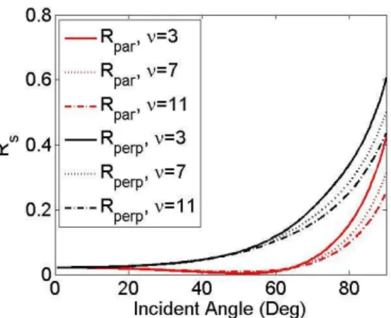
T↓ = −W R⋅ − −W R θ (14) In Eq. (14), Rs is the specular irradiance reflectance for a rough ocean surface. To evaluate Rs,
one needs to integrate the exact bidirectional reflection matrix for a rough ocean surface (see Eq. (29) in Zhai et al. [26]). Figure 1 shows the specular reflectance as a function of incident angle for three wind speeds, 3, 7, and 11 m/s. The ocean water refractive index is assumed to be 1.338. The influence of linear polarization is shown, Rpar is the irradiance reflectance when
the incident light polarization is parallel to the scattering plane, Rperp refer to the same quantity
when the polarization is perpendicular to the scattering plane. Therefore, RS values range
between Rpar and Rperp, depending on the incident light polarization. One can note that the
Fig. 1. Specular reflectance as a function of incident angle for three wind speeds, 3, 7, and 11 m/s.
It is obvious that the specular reflectance is mostly flat for incident angles smaller than 20 degrees. A rough estimation of the specular reflectance is:
0.0209 (1 0.05). s
R ≈ ⋅ ± (15)
Equation (15) is valid for angles of incidence smaller than 10 degrees and wind speeds less than 11 m/s. The uncertainty of 5% is due to variations in the polarization of the laser beam, the angle of incidence, and the wind speed. Specifically, if one needs to know a number beyond the accuracy of 5%, the angle between the plane of the linear polarization of the laser and the incident meridian plane needs to be known. While the Cox & Munk model provides a simplified approach, it allows an easy calculation. Using the recent derivation of <S2> for a space-based lidar [1,2] would only change the relationship between wind speed and wave slope variance, whereas light scattering is a function of the surface roughness state. The resultant effect would be a slight change in the applicable wind speed range.
The upward transmittance term is not mentioned in Eq. (2), whereas it is obvious that the light reflected by the subsurface water body has to cross the ocean-air interface to reach the detector. It is a direct consequence of the definition of the subsurface reflectance Ru [9] and
cannot be ignored. To accurately calculate this term, one needs to know the slope surface distribution as well as the exact upwelling radiance distribution, which is normally unknown in the lidar applications. Future lidar missions will offer more information about the subsurface term and determine if some simple assumptions can be used. To take the ocean transmittance into account, the following equation used for upward radiance tocean↑ is:
(1 ) . . ocean s foam
t↑ = −W t +W t (16) In Eq. (16), ts is the ocean interface transmittance for radiance propagating to the zenith on the
area not covered by whitecaps, and tfoam is the upward transmittance due to whitecaps for
radiance. Multiple scattering will be introduced later.
It is known that ts is only slightly dependant on wind speed [24]. Here we use the flat surface as an approximation. Hence:
2 ( ') . s s T t m θ = (17)
In Eq. (17), Ts is the irradiance transmittance for the ocean-air interface on the area not
covered by whitecaps. As we are using flat surface as an approximation, it is equal to the Fresnel irradiance transmittance which slowly changes with incident angle variations.
0.979
s
T ≈ for normal incidence angles, θ' is the underwater incident angle (θ being the angle
of refraction, following Snell's law). Tsvariations are less than 1% for θ' between 0 and 30%
but reaches 0 beyond the critical angle (48.4 degrees). m≈1.338 is the refractive index for ocean water. The m2 term is a consequence of the so called n-squared law [27]. There is a fundamental difference between transmission coefficients of irradiance and radiance which has to be taken into account within the lidar equation.
Assuming whitecaps behaves as a lambertian surface, tfoam can be easily expressed as a
function of the irradiance reflectance for foam patches Rf,eff .
, 1 . f eff foam R t π − = (18)
An assumption is made in Eq. (18) that whitecaps possess the same reflectance for upward and downward incident light. We are not aware of any underwater measurements of the irradiance reflectance of whitecaps which would confirm or disprove this assumption. We also neglected the formation of bubbles at high wind speed which could change the underwater irradiance reflectance in an unknown way. All those effects would need a better quantification, far beyond the scope of this theoretical work.
2.3.2 Subsurface reflectance value
The subsurface reflectance [9] Ru is used by all previous authors [4,5] using the lidar
subsurface equation. Using the correct treatment of ocean upward and downward transmittance (Eq. (14) and Eq. (16) allows us to revisit this formalism for the lidar equation. As will be discussed in Section 3.0, this will lead to the value of subsurface SIAB in better agreement with our previous work. We believe it is important to understand the link between
the subsurface reflectance [9] Ru and the lidar equation used for atmospheric targets. This will
be discussed in the following part. The subsurface contribution of the lidar return should be written: max max min min 2 exp( 2 ) . S s
u Tocean oceant TATM S u s u uds dS γ = ↓ ↑ β − η α
∫
∫
(19)In Eq. (19), S is the optical path (one should note that, for a lidar system, as the speed of light is lower in water than in air, the vertical resolution ∆z is reduced underwater), βu is the
underwater backscatter coefficient (m−1.sr−1), αu (m−1) is the underwater extinction coefficient,
and ηu is the multiple scattering coefficient [28]. This coefficient contains only the in-water
multiple scattering and not the air-sea interface/subsurface multiple scattering whose influence is small (around 0.5% in Eq. (21) and has been neglected here. This could however be included in this coefficient with a simple change of definition. Assuming βu and αu are
constant within the considered optical path and considering the high attenuation of water, the integrated term would be equal to [29]
max max min min exp( 2 ) . 2 S s u u u u S s u u ds dS β β η α η α − =
∫
∫
(20)Even if the two expressions are different, the backscatter coefficient in the numerator and extinction (due to absorption and scattering) in the denominator shows strong analogies with the expression derived by Morel
'
b u b
f b R
Q a+b = Q [25]. bb is the underwater backscattering
coefficient (hemispherical integration of the phase function in the backward direction), a is the underwater absorption coefficient. Q (sr) expresses the ratio of underwater radiant emittance Fu- (W.m-2) to underwater radiance Lu- (W.m-2.sr−1) and defines angular variation of
reflectance to the water’s inherent optical properties bb and a. For lidar applications, it
expresses the link between the integrated quantities bb and with the backscatter quantities βu
and αu as well as the increase of extinction when multiple scattering coefficient is present with
respect to single scattering extinction. Both Q and f' are dependent on direction and water properties. As f' and Q contain the directionality information, the formalism used by Eq. (2) using Ru instead of Eq. (20) can be used for the lidar equation, at least for a first order
approximation. To improve the accuracy, the exact similitude between integrated quantities and what is measured by the lidar will be the subject of future research.
3. Discussion
At first order, the lidar equation for an off-nadir angle θ can be expressed as
(
)
[
]
(
)
(
)
(
,)
, 2 2 5 2 , 2 , 2 , (1 ) tan ( ) exp 4 cos ( ) . cos( ) 1 (1 ) ( ) (1 ) ( ') cos( ) ( ') 1 1 1 (1 ) ( ) cos( ) 1 f eff f eff f eff ATM f eff s s u u f eff s u u W S S R W T W R W R W T R Q m rR R W R W R W R R R ρ θ π θ θ π γ θ θ θ θ θ θ π − − < > < > + = − ⋅ − − − + − − ⋅ − − − + − . (21)ris the water–air Fresnel irradiance reflectance for the whole diffuse upwelling irradiance, and is of the order of 0.48 [18]. The multiple scattering term
(
1−rRu)
takes into account thedownward, internal reflection at the interface [25]. The same formalism
(
)
, 1
f eff u
R R
− is used
for multiple scattering at the ocean-air interface where foam patches are present.
To better understand the advancement that this new equation represents, it is useful to make the comparison with Eq. (9) and Eq. (11). One can see all terms are different except the whitecaps reflectance.
Our expression of the subsurface term has never been used like this in the lidar field. Its exact value is dependant on wind speed and off-nadir angle. However we can discuss the magnitude of the modification expected with respect to the previous formalism. As it is the case for most ocean studies using lidar, and as there is still some work to be performed on the subsurface effect of whitecaps, W will be assumed equal to 0. In that case, the subsurface term
of Eq. (21) has to be compared with Ru/π at nadir. The exact value of Q depends on the lidar
incident angle, but a range between π and 5 is a reasonable estimation [24,25] for off-nadir
angle up to 30 degrees [30]. Assuming Ru = 0.01 [4] at 532 nm, the subsurface coefficient of
Eq. (21) is between 0.53 Ru/π and 0.34 Ru/π. This lower value is consistent with our analysis
of CALIPSO ocean surface echo [2] in which the subsurface contribution is not significant. Previous studies using large off nadir angles [5,17] did not find values of subsurface return lower than that given by Eq. (2). However, as those studies were using a 2π factor instead of 4π in the specular reflectance term, this lowers the relative difference between the subsurface and specular term and the global factor 2 bias can come from the uncertainty of the lidar calibration, and the wind speed estimation or surface roughness model as the Cox and Munk model [16] is an approximation [1].
Here we find that the differences range from 89% (0.53 Ru/π) to 194% (0.34 Ru/π).
It is recommended that, for future lidar applications, Eq. (21) should be used. Additional research will need to be conducted to further improve the accuracy. Specifically, improvements to Eq. (21) would include the probability of slope distribution in the cross and
upwind components [18], as well as to gain a better understanding of the subsurface term given by Eq. (20). There is also a need to better assess the large uncertainties associated with the lidar return of foam patches and their effect on subsurface lidar returns.
4. Conclusion
We revisited the formalism to be used for the analysis of the lidar ocean surface and subsurface returns (Eq. (21). The previous formalism had weaknesses in specular return angular dependency and would lead to an overestimation of the subsurface contribution by a factor of two to three. This improved lidar equation is more consistent with the latest advances in radiative transfer theory. This advancement will have a direct impact on the scientific outcome of future space-based lidar missions, and will more accurately determine some of the coefficients critical to ocean color research and their directional dependencies.
Appendix A
The power received by the telescope can be expressed as in the classical lidar equation formalism (see Eq. (7).23 of [31] for elastic scattering when the wavelength of observation is the same as that of the laser)
2 2 ( ) L ( ) ( ). r ATM C P R R T R R β = (A.1)
In Eq. (A.1), Pr is the optical power (in W) collected by the lidar receiver system
(telescope). CL is the lidar system parameter commonly referred as the lidar constant (in
W.m3.sr). R is the range (in m) between the lidar transceiver system and the scattering target
(molecule, particle, surface). β is the backscatter coefficient (m−1.sr−1). TATM = exp(-τATM/µ) is
the one-way transmittance of the atmosphere for the laser light and τATM is the vertical
atmospheric optical depth. As we will discuss the surface return, which is at a specific and well determined range, the dependence of the different variables with R will not been shown in the following equations.
By definition, the lidar constant CL is
0 .
2
L t
c
C = E A (A.2)
In Eq. (A.2), At is the telescope area (m2), c the speed of light (m.s−1) and E0 the laser
energy emission (J). Here a perfect efficiency of the receiver is assumed. It is also assumed a perfect transceiver alignment and all emitted light is collected by the telescope (i.e. the telescope field of view is larger than the laser beam divergence and the diffraction occurs far enough from the lidar system so there is no overlap problem).
When studying the surface, it is necessary to write the lidar equation in a different way. The power received by the telescope coming from the surface is equal to
exp ATM . r r t G P L A τ µ = Ω − (A.3)
Lr is the upward radiance (W.m
−2
.sr−1) at the surface level and ΩG is the solid angle (sr) from
which the surface is seen from the telescope (subscript G for ground). This solid angle is by definition:
2 . G G A R µ Ω = (A.4)
AG is the area of the laser footprint. It is the real area on the ground, so it is a function of µ but
using the real area is the standard way to define the solid angle of the surface. The BRDF of the surface is by definition [11–13]
0 . r BRDF L F π ρ µ = (A.5)
F0 (W.m−2) is the incident flux per unit area perpendicular to the incident beam.
Combining (A.4) and (A.5) with (A.3) we get
0 2 exp . BRDF G ATM r t F A P A R µ ρ µ τ π µ = − (A.6)
F0 can also be written as the laser emitting power P0 per unit area projected perpendicular to
the incident beam and attenuated by the atmospheric absorption and scattering
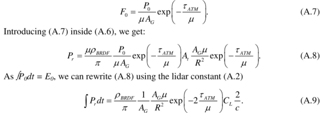
0 0 exp . ATM G P F A τ µ µ = − (A.7)
Introducing (A.7) inside (A.6), we get:
0 2 exp G exp . BRDF ATM ATM r t G P A P A A R µ µρ τ τ π µ µ µ = − − (A.8)
As ∫P0dt = E0, we can rewrite (A.8) using the lidar constant (A.2)
2 1 2 exp 2 . G BRDF ATM r L G A P dt C A R c µ ρ τ π µ = −
∫
(A.9)As the surface level is well defined there is no time dependency on the right side of Eq. (A.9) and using dt = 2dR/c we can express the BRDF as a function of lidar surface integrated attenuated backscatter (SIAB) coefficient γ (sr−1) as in Eq. (A.10)
2 exp 2 . 2 r BRDF ATM L P R c dt C ρ τ γ µ π µ = = −
∫
(A.10)Coming back to its definition, the SIAB is (for a scatterer at a given altitude) the ratio of the energy collected by the telescope (∫Prdt = Er) per unit of telescope solid angle (Ωt = At/R2)
on the laser energy emission E0 as written in Eq. (A.11).
0 . r t E E γ = Ω (A.11) Appendix B: Index
Table B.1. Index of different terms used in this manuscript Index of the different terms used in this study Variable Link with other
variables
Definition Unit Notes
θ Incident angle of light with respect to the zenith
rad. For this study, θ mainly refers to the lidar off-nadir angle
µ cos (θ) Cosine of incident angle of light No unit θ' Under water incident angle of light
with respect to the zenith
rad. Conterpart of θ following Snell's law
Table B.2. Index of different terms used in this manuscript (continued) Index of the different terms used in this study
Variable Link with other variables
Definition Unit Notes
ocean R 0 r F F µ
Irradiance reflectance of the ocean surface No unit Rf, eff , 0 f eff F F µ
Irradiance reflectance of foam patches No unit RS 0 S F F µ
Irradiance reflectance of ocean rough surface (specular return)
No unit Ru 0 u F F µ − −
Irradiance reflectance of ocean just below the surface level (underwater)
No unit
Fr Radiant emittance of the ocean at
surface level W.m
−2
Ff,eff radiant emittance of foam patches W.m−2
FS radiant emittance of ocean rough
surface
W.m−2 Fu- radiant emittance of the ocean just
below the surface level W.m
−2
F0 Incident flux per unit area
perpendicular to the incident beam at surface level
W.m−2 It is the (atmospheric attenuated) solar constant for passive measurements
F0- incident flux per unit area perpendicular
to the incident beam just below the surface level
W.m−2
W Fraction of the surface covered with whitecaps
No unit
foam
T↓ 1-W.Rf,eff downward irradiance transmittance of
foam patches at surface level
No unit
ocean
T↓ Oceanic transmittance at surface leveldownward irradiance No unit
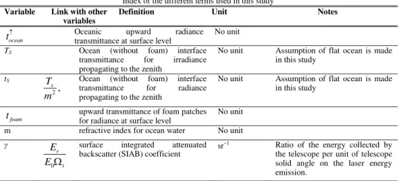
Table B.3. Index of different terms used in this manuscript (continued) Index of the different terms used in this study
Variable Link with other variables
Definition Unit Notes
ocean
t↑ Oceanic transmittance at surface levelupward radiance No unit
TS Ocean (without foam) interface
transmittance for irradiance propagating to the zenith
No unit Assumption of flat ocean is made in this study tS 2, s T m
Ocean (without foam) interface transmittance for radiance propagating to the zenith
No unit Assumption of flat ocean is made in this study
foam
t upward transmittance of foam patches for radiance at surface level
No unit
m refractive index for ocean water No unit
γ 0 r t E EΩ
surface integrated attenuated backscatter (SIAB) coefficient sr
−1 Ratio of the energy collected by
the telescope per unit of telescope solid angle on the laser energy emission.
γS contributions of the specular return to
the surface integrated backscatter coefficient
sr−1
γf contributions of the foam patches to
the surface integrated backscatter coefficient
sr−1
γu contributions of the subsurface to the
surface integrated backscatter coefficient sr−1 ρBRDF 0 r L F π µ
Bidirectionnal reflectance distribution function (BRDF)
sr−1 BRDF is a function of the angle of incidence and reflection
Lr radiance of the surface W.m−2.sr−1
Lf,eff radiance of the surface by foam
patches
W.m−2.sr−1 LS radiance of the surface due to
specular return
W.m−2.sr−1 Lu- radiance of of the ocean just below
the surface level
W.m−2.sr−1 ρ Fresnel reflectance coefficient at
nadir angle
sr−1 <S2> variance of the wave slope
distribution
No unit Also called mean square slope (MSS)
p(ςx, ςy) probability of slopes of waves No unit ςx and ςy are the slopes along- and
cross-wind directions. Table B.4. Index of different terms used in this manuscript (continued)
Index of the different terms used in this study Variable Link with other
variables
Definition Unit Notes
v wind speed m.s−1 measured at 12 meters above the
ocean surface βu underwater backscatter coefficient m−1.sr−1
αu underwater extinction coefficient m−1
ηu Underwater multiple scattering
coefficient No unit Q u u F L − −
ratio of underwater radiant emittance to underwater radiance
sr
f' empirical coefficient No unit It links the irradiance reflectance
to the water inherent optical properties bb and a
bb underwater backscattering coefficient m−1 hemispherical integration of the
phase function in the backward direction
a underwater absorption coefficient m−1
r water–air Fresnel reflection for the whole diffuse upwelling irradiance No unit
d
P optical power collected by the lidar receiver (telescope)
W
CL lidar system parameter W.m3.sr commonly referred as the lidar
constant
R range between the lidar transceiver system and the scattering target (molecule, particle, surface)
m c is the speed of light t is the time Er ∫Prdt energy collected by the telescope,
coming from the surface
J Pr (W) is the power collected by
the lidar receiver system, coming from the surface
Ωt Telescope solid angle seen from the
surface
sr
E0 ∫P0dt Laser energy emission (laser impulse) J P0 (W) is the power emitted by
the lidar system (laser impulse power)
TATM exp(-τATM/µ) one-way transmittance of the atmosphere
No unit τATM Atmospheric vertical optical depth No unit
S Optical path m
Acknowledgments
This work has been supported by NASA Postdoctoral Program (NPP) at NASA Langley Research Center administered by Oak Ridge Associated Universities. Science Systems and Applications Inc. (SSAI) is greatly acknowledged for their support. We would like to thank the two anonymous reviewers for suggesting corrections and improvements to the manuscript.