HAL Id: hal-00317718
https://hal.archives-ouvertes.fr/hal-00317718
Submitted on 3 Nov 2004
HAL is a multi-disciplinary open access
archive for the deposit and dissemination of
sci-entific research documents, whether they are
pub-lished or not. The documents may come from
teaching and research institutions in France or
abroad, or from public or private research centers.
L’archive ouverte pluridisciplinaire HAL, est
destinée au dépôt et à la diffusion de documents
scientifiques de niveau recherche, publiés ou non,
émanant des établissements d’enseignement et de
recherche français ou étrangers, des laboratoires
publics ou privés.
Solar wind velocity at solar maximum: A search for
latitudinal effects
B. Bavassano, R. d’Amicis, R. Bruno
To cite this version:
B. Bavassano, R. d’Amicis, R. Bruno. Solar wind velocity at solar maximum: A search for
lat-itudinal effects. Annales Geophysicae, European Geosciences Union, 2004, 22 (10), pp.3721-3727.
�hal-00317718�
SRef-ID: 1432-0576/ag/2004-22-3721 © European Geosciences Union 2004
Annales
Geophysicae
Solar wind velocity at solar maximum: A search for latitudinal
effects
B. Bavassano, R. D’Amicis, and R. Bruno
Istituto di Fisica dello Spazio Interplanetario (C.N.R.), Roma, Italy
Received: 5 February 2004 – Revised: 29 June 2004 – Accepted: 2 July 2004 – Published: 3 November 2004
Abstract. Observations by Ulysses during its second
out-of-ecliptic orbit have shown that near the solar activity maxi-mum the solar wind appears as a highly variable flow at all heliolatitudes. In the present study Ulysses data from po-lar latitudes are compared to contemporary ACE data in the ecliptic plane to search for the presence of latitudinal effects in the large-scale structure of the solar wind velocity. The investigated period roughly covers the Sun’s magnetic po-larity reversal. The Ulysses-ACE comparison is performed through a multi-scale statistical analysis of the velocity fluc-tuations at scales from 1 to 64 days. The results indicate that, from a statistical point of view, the character of the wind ve-locity structure does not appear to change remarkably with latitude. It is likely that this result is characteristic of the particular phase of the solar magnetic cycle.
Key words. Interplanetary physics (interplanetary magnetic
fields; solar wind plasma; sources of the solar wind)
1 Introduction
The three-dimensional structure of the solar wind observed by Ulysses at high solar activity during its second out-of-ecliptic orbit is completely different from that seen at low activity along the first orbit (McComas et al., 2003). In fact, in the latter case the solar wind is characterized by a bimodal structure (McComas et al., 1998), with a steady, fast wind at high latitudes and a slower and more variable wind at low latitudes. Conversely, at high solar activity highly variable flows are observed at all latitudes and the wind structure ap-pears to be a complicated mixture of flows coming from a variety of sources (McComas et al., 2002a,b, 2003; Neuge-bauer et al., 2002; Fujiki et al., 2003; Riley et al., 2003).
This state with variable flows at all heliographic latitudes is a short-lived feature of the heliosphere. After the reversal of the solar magnetic field (Jones et al., 2003), a recovery of the wind’s bimodal structure begins quite soon. Ulysses ob-servations along the northern leg of the second orbit already Correspondence to: B. Bavassano
indicate a robust return of the high-latitude fast wind (Mc-Comas et al., 2002b). The only opportunity to investigate the properties of the high-latitude solar wind around solar maxi-mum before the recovery of a bimodal structure is offered by the Ulysses plasma measurements along the second orbit’s southern leg (it is worth recalling that in its out-of-ecliptic orbits Ulysses is first travelling in the Southern Hemisphere, then in the Northern one, with a fast latitudinal scan from south to north through the perihelion).
In the present study we will analyse a subset of Ulysses data from this southern polar phase, more precisely the time interval during which the spacecraft moves from 50◦S to the
highest latitude (80.2◦S) and then back to 50◦S. We will perform a comparison with data collected at the same time by ACE, which is orbiting in the ecliptic plane around the Sun-Earth L1 libration point (∼0.01 AU, astronomical unit, sunward of the Earth). Our aim is that of looking for the pres-ence of latitudinal trends in the large-scale structure of the solar wind velocity near the solar activity maximum. While a latitudinally ordered structure, as that observed at low so-lar activity, is surely absent, it might well be that less obvi-ous latitudinal trends are present in the velocity pattern. Our Ulysses-ACE comparison is based on a statistical approach, a complementary view with respect to studies such as that by Elliott et al. (2003), which was based on the use of a deter-ministic model.
2 Data Analysis
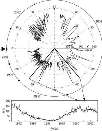
The data used in the present study are daily averages of the solar wind velocity magnitude ˇ as measured by the SWOOPS and SWEPAM plasma analyzers aboard Ulysses and ACE, respectively (for both experiments D. J. McComas is the principal investigator). As mentioned above, the anal-ysed Ulysses data are from southern latitudes poleward of 50◦S, as displayed in Fig. 1. Here at the top we give a po-lar plot of ˇ versus the heliographic latitude for years 1998 to 2002. The angular sector delimited by thick lines indi-cates the investigated interval, from day 88 (2000) to day 63 (2001). It just corresponds to a maximum of the solar activity cycle, as evidenced by the sunspot numbers shown
3722 B. Bavassano et al.: Solar wind velocity at solar maximum 30 60 90 60 30 0 -30 -60 -90 -60 -30 300 600 900 (km/s) V 1992 1994 1996 1998 2000 2002 0 50 100 150 200 year ssn 1998 1999 2000 2001 2002
Fig. 1. A polar plot of the solar wind velocity ˇ vs. heliographic
latitude is shown at the top for years 1998 to 2002. Dots along the outermost circle mark the beginning of each year, with time in-creasing anticlockwise from the leftmost dot (see arrowhead). The bottom panel gives solar sunspot numbers (ssn) in terms of monthly and smoothed values (thin and thick line, respectively) for a 12-year interval starting in 1991. The angular sector indicated by thick lines in the top plot and the thick segment in the bottom plot identify the analysed interval. A narrower sector delimited by lighter lines identifies a very-high-latitude subinterval, see text.
in the bottom plot (see the thick segment indicated by ar-rows). Moreover, Ulysses observations from the latitudinal scan around perihelion (McComas et al., 2002b) indicate that the polarity reversal of the solar magnetic field occurs from early 2000 to early 2001 (Jones et al., 2003), namely just during the time interval investigated here. It should also be mentioned that this same interval has already been the object of a study by McComas et al. (2002a) from the point of view of the wind solar sources.
In Fig. 2 the wind velocity ˇ and the spacecraft coordi-nates (heliocentric distance ˚ and heliographic latitude λ) are plotted versus time for the investigated interval. The interval is thirteen solar rotations long, as seen by Ulysses, with ˚ decreasing from 3.76 to 1.62 AU and λ varying from −49.8◦to −80.2◦and again to −49.8◦. The velocity profile shown in Fig. 2 is quite variable, with slow flows close to ∼300 km/s and peaks at ∼700 km/s. As indicated by Mc-Comas et al. (2002a), the velocity peaks observed during this interval generally are related to flows originating from small coronal holes. A remarkable feature in Fig. 2 is that
300 400 500 600 700 ULYSSES (km/s) V 1.5 2 2.5 3 3.5 4 2000 (AU) R 100 150 200 250 300 350 34 -80o -70o -60o -50o 2001 day of year VHL interval
Fig. 2. The solar wind velocity ˇ and the Ulysses heliocentric
dis-tance ˚ and heliographic latitude λ are plotted vs. time for the in-vestigated interval. Dashed lines delimit an interval at very high lat-itudes (VHL), where the ˇ curve does not exhibit prominent peaks.
ˇ does not exhibit any major peak for quite a long period of time (approximately from day 200, 2000 to 45, 2001), corresponding roughly to latitudes poleward of 60◦S. This peculiarity has led us to focus our study on this subinterval at higher latitudes. Thus, in addition to the full interval of thirteen solar rotations mentioned above, in the following we will also analyse a shorter interval spanning from day 216, 2000 ( ˚=3.05 AU, λ=−64.89◦) to day 37, 2001 ( ˚=1.78 AU,
λ=−62.25◦), with a total duration of seven rotations. It is highlighted in Fig. 2 by dashed lines and labelled as VHL (very-high-latitude) interval. In the top plot of Fig. 1 the VHL interval corresponds to the angular sector delimited by light lines.
A multi-scale statistical analysis of the velocity varia-tions (e.g. see Burlaga and Forman, 2002; Burlaga et al., 2003) has been used to characterize the structure of the so-lar wind at time scales above ∼1 day. The procedure is quite simple. First, from daily averages of the wind ve-locity magnitude ˇ, time series of the veve-locity differences at given time lags τ have been obtained. Choosing τ equal to 2n days for n=0, 1, 2, 3, 4, 5, and 6, seven time series dV n≡dV n(t )=V (t +2n)−V (t ) have been derived. Then, for each time series (i.e. each time lag), the occurrence fre-quency distribution of the dV n(t ) population and the corre-sponding values of mean, standard deviation, skewness, and kurtosis, have been computed. The values at the different lags of these statistical quantities provide an overview of the basic features of the solar wind velocity structure.
VHL interval 300 400 500 600 700 ULYSSES (km/s) V -200 0 200 (km/s) dV1 2-day -200 0 200 (km/s) dV2 4-day -200 0 200 2000 (km/s) dV4 16-day 100 150 200 250 300 350 34 -200 0 200 2001 (km/s) day of year dV6 64-day
Fig. 3. From top to bottom: solar wind velocity ˇ and velocity
dif-ferences dV 1, dV 2, dV 4, and dV 6 (at time lags of 2, 4, 16, and 64 days, respectively) versus time for the analysed Ulysses data. A bar on top indicates the VHL (Very-High-Latitude) interval.
As is well known, the skewness measures the asymme-try of a distribution and the kurtosis measures its peakedness (relative to a Gaussian distribution). For a Gaussian distri-bution the skewness is obviously 0, while the kurtosis, as defined by the ratio of the fourth to the squared second mo-ment of the distribution, has a value of 3. The definition used here gives an unbiased estimate of the kurtosis (essentially with subtraction of the factor 3), thus in the present paper the kurtosis is 0 for a Gaussian distribution.
3 Velocity differences and frequency distributions
3.1 Ulysses observations
The velocity differences dV 1, dV 2, dV 4, and dV 6 (at time lags of 2, 4, 16, and 64 days, respectively) for the analysed Ulysses data are plotted versus time in Fig. 3 (second to fifth panel from top). In the top panel the ˇ daily averages, already shown in Fig. 2, are reported for easier reference.
At small scales the velocity differences are relatively small and spiky (e.g. see the dV 1 curve), with the exception of values coming from sharp gradients of ˇ. At larger scales the
0.002 0.01 0.02 0.1 0.2 ULYSSES F dV0 1-day dV3 8-day 0.002 0.01 0.02 0.1 0.2 F dV1 2-day dV4 16-day -400 -200 0 200 400 0.002 0.01 0.02 0.1 0.2 (km/s)dV F dV2 4-day -400 -200 0 200 400 (km/s)dV dV6 64-day
Fig. 4. The occurrence frequency F (in a logarithmic scale) of
the Ulysses velocity differences dV 0, dV 1, dV 2, dV 3, dV 4, and dV6 is shown by histograms in the different panels. The solid curves give Gaussian distributions as computed from the observed values of mean and standard deviation.
curves exhibit smoother variations of larger amplitude. This is similar to the findings of Burlaga et al. (2003).
The occurrence frequency F of the Ulysses velocity differ-ences dV 0, dV 1, dV 2, dV 3, dV 4, and dV 6 (correspond-ing to 1−, 2−, 4−, 8−, 16−, 64−day time lags) is shown by histograms in the panels of Fig. 4. The curves indicate Gaussian distributions as obtained from the observed values of mean and standard deviation (i.e. they are not the result of a fit procedure). It is clearly seen that the distribution width increases going from 1− to 8−day lags, then remains almost constant. At a first glance the histograms appear qualitatively closer to a Gaussian curve at large scales. These points will be thoroughly discussed in Sect. 4.
3.2 ACE observations
As mentioned in the Introduction, our analysis is based on the comparison between Ulysses data from the Southern Hemi-sphere (latitudes poleward of 50◦S) and contemporary data by ACE on the ecliptic plane. The analysed ACE interval spans from day 77, 2000 to day 61, 2001. As for Ulysses,
3724 B. Bavassano et al.: Solar wind velocity at solar maximum 400 500 600 700 800 ACE (km/s) V -200 0 200 (km/s) dV1 2-day -200 0 200 (km/s) dV2 4-day -200 0 200 2000 (km/s) dV4 16-day 100 150 200 250 300 350 34 -200 0 200 2001 (km/s) day of year dV6 64-day
Fig. 5. Solar wind velocity ˇ and velocity differences dV 1, dV 2,
dV4, and dV 6 for the analysed ACE interval, in the same format of Fig. 3. A bar on top indicates the ACE interval that corresponds to the Ulysses VHL interval.
this interval has a total length of thirteen solar rotations. The time changes with respect to the Ulysses data base are to ac-count for a slightly different duration of the solar rotation as seen by ACE (in a halo orbit at L1) and by Ulysses (in a deep space orbit). Moreover, a time delay to allow for solar wind propagation from ACE (at 1 AU) to Ulysses distances (3.76 to 1.62 AU) has been taken into account, although this kind of approach may be questionable for the case of largely sep-arated spacecraft in a high-solar-activity wind (e.g. see Elliot et al., 2003; Riley et al., 2003).
The solar wind velocity (daily averages) for the analysed ACE interval is shown in the top panel of Fig. 5. Similarly to the Ulysses observations, the ACE velocity profile is quite variable. A bar on top indicates the ACE interval (days 211, 2000 to 33, 2001) that corresponds to the Ulysses VHL in-terval. As in Fig. 3, the second to fifth panels (from top) give the velocity differences dV 1, dV 2, dV 4, and dV 6. At a first glance, the curves at small lags seem to indicate an enhanced variability of the ACE data as compared to Ulysses data.
The frequency histograms of the ACE velocity differences are given in Fig. 6, in the same format of Fig. 4. As for Ulysses, going from 1− to 8−day lags the distribution width
0.002 0.01 0.02 0.1 0.2 ACE F dV0 1-day dV3 8-day 0.002 0.01 0.02 0.1 0.2 F dV1 2-day dV4 16-day -400 -200 0 200 400 0.002 0.01 0.02 0.1 0.2 (km/s)dV F dV2 4-day -400 -200 0 200 400 (km/s)dV dV6 64-day
Fig. 6. Frequency histograms for the ACE velocity differences, in
the same format of Fig. 3.
increases, then (i.e. at larger lags) this trend disappears. Moreover, it is easily seen that at small lags the ACE his-tograms are wider than those for Ulysses.
4 Moments
As already mentioned, a simple way to get an overall scription of the dV n distribution properties and of their de-pendence upon scale (i.e. the time lag τ ) is that of looking at the behaviour of their moments.
In Fig. 7 the dependence on τ of mean, standard deviation, skewness, and kurtosis is shown separately for Ulysses (solid lines) and ACE (dashed lines) data. Regarding the mean (top panel), it is seen to be close to zero at all scales for Ulysses. For ACE this does not hold at time lags of 32 and 64 days. However, the difference from zero, in absolute value, does not go beyond ∼10% of the standard deviation. The standard deviation (second panel from top) roughly ranges from 35 to 120 km/s for Ulysses and from 60 to 130 km/s for ACE. With the exception of τ =16, the standard deviation is always higher for ACE data. Skewness and kurtosis (third and fourth panels) indicate a close-to-Gaussian behaviour for ACE at
-40 0 40 Mean (km/s) ULYSSES ACE 40 80 120 St. Dev. (km/s) -2 0 2 Skewness 1 2 4 8 16 32 64 0 5 10 (days) Kurtosis
Fig. 7. The dependence of mean, standard deviation, skewness, and
kurtosis on the time lag τ is shown separately for Ulysses (solid lines) and ACE (dashed lines) data. Error bars are given for skew-ness and kurtosis (in some cases errors are smaller than the marker size).
all scales. In contrast, non-Gaussian features come out for Ulysses at τ <8, with a kurtosis value of ∼11 at the smallest scale.
The presence of non-Gaussian features in the Ulysses dis-tributions is a relevant point and needs to be carefully inves-tigated. From dV 1, dV 2 and dV 3 Ulysses data plotted in Fig. 3 it clearly appears that the values outside the core of the distribution mainly come from the two major ˇ peaks (top panel) near days 193 (2000) and 47 (2001). The VHL inter-val, covering the Ulysses trajectory phase poleward of ∼65◦, falls just between these two peaks. From Fig. 2 it can be argued that the solar wind conditions above the Sun’s polar regions are better described by data from the VHL interval, rather than from the entire examined interval. Then, we have focused our analysis on the VHL interval of Ulysses data and on the corresponding ACE data interval (see Fig. 5 on top). The new values of mean, standard deviation, skewness, and kurtosis are plotted in Fig. 8. It clearly appears that at all scales the Ulysses values for skewness and kurtosis are now close to zero (and close to the corresponding ACE values). Thus, the above indication about non-Gaussian features does not hold for VHL data.
-40 0 40 Mean (km/s) ULYSSES ACE VHL interval 40 80 120 St. Dev. (km/s) -2 0 2 Skewness 1 2 4 8 16 32 64 0 5 10 (days) Kurtosis
Fig. 8. Mean, standard deviation, skewness, and kurtosis vs. time
lag τ for the VHL interval, in the same format of Fig. 7.
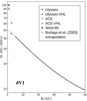
Regarding the mean and standard deviation, Fig. 8 con-firms that mean values different from zero come out at large τ (up to 25% of the standard deviation for ACE, perhaps an effect of data gaps) and that at all scales the standard devia-tion values for ACE are higher than those for Ulysses. Since Ulysses and ACE measurements come from different radial distances, the question arises if the standard deviation de-crease at Ulysses may be ascribed to a radial effect. This point is addressed by Fig. 9. Here we plot the dV 1 standard deviations for Ulysses (filled triangles, down for the whole data interval and up for the VHL interval), ACE (triangles, down and up as for Ulysses), and Wind (filled square). Av-erage radial distances are used for Ulysses values (2.74 and 2.43 AU for the whole data set and the VHL interval, respec-tively). The Wind-95 value refers to a thirteen solar rotation interval in 1995 (days 12 to 362). The solid curve shown in the figure is from Burlaga et al. (2003). It has been derived by applying a model developed by Wang et al. (2002) (see more references in the paper by Burlaga et al.) to describe the so-lar wind evolution in the outer heliosphere. Using 1995 Wind data as input to the model at 1 AU, Burlaga et al. (2003) de-termined the velocity structure from 5 to 95 AU at steps of 5 AU and computed the distribution moments for dV 1. The curve is an exponential fit to the standard deviation values
ob-3726 B. Bavassano et al.: Solar wind velocity at solar maximum 0 10 20 30 40 50 10 20 30 40 50 60 70 80 90 100 R (AU) St. Dev. (km/s) Ulysses Ulysses-VHL ACE ACE-VHL Wind-95 Burlaga et al. (2003) extrapolation
dV1
Fig. 9. The standard deviation as measured by Ulysses and by
near-Earth spacecraft (ACE and Wind). The solid curve is from Burlaga et al. (2003), dots indicate an extrapolation to 1 AU.
tained with this procedure. It is immediately apparent from Fig. 9 that the ACE and Wind standard deviations (triangles and filled square) are much higher than the extrapolation to 1 AU (dotted curve) of the 5–95 AU fit. Thus, from 1 to 5 AU the standard deviation decrease has to be much faster than be-yond 5 AU. The Ulysses standard deviations (filled triangles) appear to be in reasonable agreement with this ecliptic radial trend. Then, the outcome of a lower standard deviation at Ulysses with respect to ACE is probably a radial rather than a latitudinal effect. It must be stressed, however, that all this holds only for dV 1. The extension to other scales is just a hypothesis. A last comment about Fig. 9, though marginal for the present paper, is that the difference between ACE and Wind standard deviations at 1 AU is small, though they refer to periods at completely different phases of the solar cycle (see, in the bottom plot of Fig. 1, the sunspot number for 1995 and 2000–2001 periods). In other words, the solar ac-tivity does not appear to affect the solar wind variability as measured by dV 1.
5 Conclusions
Ulysses data from southern latitudes greater than 50◦have been compared to contemporary ACE data in the ecliptic plane to search for the presence of latitudinal effects in the large-scale structure of the solar wind velocity. The study refers to high solar activity conditions, when the solar wind appears as a highly variable flow at all latitudes. The
compar-ison is performed by using a multi-scale statistical analysis of the velocity differences at scales from 1 to 64 days.
The skewness and kurtosis behaviours for the whole inter-val investigated indicate a close-to-Gaussian behaviour for ACE at all the scales. In contrast, non-Gaussian features come out for Ulysses at the small scales (τ <8 days). But, if we focus the analysis on the VHL (Very-High-Latitude) interval, this last result does not appear to be confirmed. In fact, for Ulysses VHL data, both skewness and kurtosis are close to 0 (and close to the ACE values) at all the scales. Solar wind conditions above the Sun’s poles appear better described by data from the VHL interval rather than from the whole interval examined. Then, we are led to conclude that at the examined scales the distributions of the velocity differ-ences have a Gaussian character for both polar and ecliptic solar wind.
Differences between Ulysses and ACE are observed for the standard deviation level, with ACE values higher than those for Ulysses. We have shown that the Ulysses standard deviations are in reasonable agreement with the overall radial variation observed in the ecliptic plane. Then, the Ulysses-ACE differences probably are a radial rather than latitudinal effect.
In conclusion, from a statistical point of view, the charac-ter of the solar wind velocity structure at large scales around solar maximum does not appear to change remarkably with latitude. It should be recalled that the time interval investi-gated here roughly corresponds to that of the polarity reversal of the solar magnetic field (Jones et al., 2003). Under such conditions it is not surprising that latitude does not play any relevant role in shaping the solar wind. However, as already underlined in the Introduction, the investigated interval is a unique, short-lived period in the context of the entire solar activity cycle. During most of the cycle the wind velocity exhibits a well developed latitudinal pattern.
As a final remark it should be stressed again that our con-clusions belong to the statistical domain. When the Ulysses-ACE comparison is done for specific individual structures (Elliott et al., 2003), it comes out that at latitude separations above ∼30◦no correlation is left.
Acknowledgements. The use of data from the Ulysses/SWOOPS
and ACE/SWEPAM plasma analyzers (principal investigator D. J. McComas, Southwest Research Institute, San Antonio, Texas, USA) is gratefully acknowledged. The data have been obtained through the NASA World Data Center A for Rockets and Satel-lites (Goddard Space Flight Center, Greenbelt, Maryland, USA). Ruth Skoug has kindly made available ACE data for the Bastille-day event. Solar sunspot data are from the World Data Center for the Sunspot Index, Royal Observatory of Belgium (Brussels, Bel-gium). The present work has been supported by the Italian Space Agency (ASI) under contract IR/064.
Topical Editor R. Forsyth thanks two referees for their help in evaluating this paper.
References
Burlaga, L.F. and Forman, M. A.: Large-scale speed fluctuations at 1 AU on scales from 1 h to ≈1 year: 1999 and 1995, J. Geophys. Res., 107(A11), 1403, doi:10.1029/2002JA009271, 2002. Burlaga, L. F., Wang, C., Richardson, J. D., and Ness, N. F.:
Evolution of the multiscale statistical properties of corotating streams from 1 to 95 AU, J. Geophys. Res., 108(A7), 1305, doi:10.1029/2003JA009841, 2003.
Elliott, H. A., McComas, D. J., and Riley, P.: Latitudinal extent of large-scale structures in the solar wind, Ann. Geophys., 21, 1331–1339, 2003.
Fujiki, K., Kojima, M., Tokumaru, M., Ohmi, T., Yokobe, A., Hayashi, K., McComas, D. J., and Elliott, H. A.: How did the so-lar wind structure change around the soso-lar maximum? From in-terplanetary scintillation observation, Ann. Geophys., 21, 1257– 1261, 2003.
Jones, G. H., Balogh, A., and Smith, E. J.: Solar magnetic field reversal as seen at Ulysses, Geophys. Res. Lett., 30(19), 8028, doi:10.1029/2003GL017204, 2003.
McComas, D. J., Bame, S. J., Barraclough, B. L., Feldman, W. C., Funsten, H. O., Gosling, J. T., Riley, P., Skoug, R., Balogh, A., Forsyth, R., Goldstein, B. E., and Neugebauer, M.: Ulysses re-turn to the slow solar wind, Geophys. Res. Lett., 25, 1–4, 1998.
McComas, D. J., Elliot, H. A., and von Steiger, R.: Solar wind from high-latitude coronal holes at solar maximum, Geophys. Res. Lett., 29(9), doi:10.1029/2001GL013940, 2002a.
McComas, D. J., Elliot, H. A., Gosling, J. T., Reisenfeld, D. B., Skoug, R. M., Goldstein, B. E., Neugebauer, M., and Balogh, A.: Ulysses’ second fast-latitude scan: Complexity near solar maximum and the reformation of polar coronal holes, Geophys. Res. Lett., 29(9), doi:10.1029/2001GL014164, 2002b.
McComas, D. J., Elliott, H. A., Schwadron, N. A., Gosling, J. T., Skoug, R. M., and Goldstein, B. E.: The three-dimensional solar wind around solar maximum, Geophys. Res. Lett., 30(10), 1517, doi:10.1029/2003GL017136, 2003.
Neugebauer, M., Liewer, P. C., Smith, E. J., Skoug, R. M., and Zurbuchen, T. H.: Sources of the solar wind at so-lar activity maximum, J. Geophys. Res., 107(A12), 1488, doi:10.1029/2001JA000306, 2002.
Riley, P., Miki´c, Z., and Linker, J. A.: Dynamical evolution of the inner heliosphere approaching solar activity maximum: inter-preting Ulysses observations using a global MHD model, Ann. Geophys., 21, 1347–1357, 2003.
Wang, C., Richardson, J. D., and Gosling, J. T.: A numerical study of the evolution of the solar wind from Ulysses to Voyager 2, J. Geophys. Res., 105, 2337–2344, 2000.