HAL Id: hal-00304591
https://hal.archives-ouvertes.fr/hal-00304591
Submitted on 1 Jan 2001HAL is a multi-disciplinary open access archive for the deposit and dissemination of sci-entific research documents, whether they are pub-lished or not. The documents may come from teaching and research institutions in France or abroad, or from public or private research centers.
L’archive ouverte pluridisciplinaire HAL, est destinée au dépôt et à la diffusion de documents scientifiques de niveau recherche, publiés ou non, émanant des établissements d’enseignement et de recherche français ou étrangers, des laboratoires publics ou privés.
Disaggregation of spatial rainfall fields for hydrological
modelling
N. G. Mackay, R. E. Chandler, C. Onof, H. S. Wheater
To cite this version:
N. G. Mackay, R. E. Chandler, C. Onof, H. S. Wheater. Disaggregation of spatial rainfall fields for hydrological modelling. Hydrology and Earth System Sciences Discussions, European Geosciences Union, 2001, 5 (2), pp.165-173. �hal-00304591�
Disaggregation of spatial rainfall fields for hydrological
modelling
N.G. Mackay
1, R.E. Chandler
2, C. Onof
1*and H.S. Wheater
11Imperial College of Science, Technology and Medicine, Department of Civil and Environmental Engineering, London SW7 2BU 2 University College London, Department of Statistical Science, London WC1E 6BT
*Email for corresponding author: [email protected]
ABSTRACT
Meteorological models generate fields of precipitation and other climatological variables as spatial averages at the scale of the grid used for numerical solution. The grid-scale can be large, particularly for GCMs, and disaggregation is required, for example to generate appropriate spatial-temporal properties of rainfall for coupling with surface-boundary conditions or more general hydrological applications. A method is presented here which considers the generation of the wet areas and the simulation of rainfall intensities separately. For the first task, a nearest-neighbour Markov scheme, based upon a Bayesian technique used in image processing, is implemented so as to preserve the structural features of the observed rainfall. Essentially, the large-scale field and the previously disaggregated field are used as evidence in an iterative procedure which aims at selecting a realisation according to the joint posterior probability distribution. In the second task the morphological characteristics of the field of rainfall intensities are reproduced through a random sampling of intensities according to a beta distribution and their allocation to pixels chosen so that the higher intensities are more likely to be further from the dry areas. The components of the scheme are assessed for Arkansas-Red River basin radar rainfall (hourly averages) by disaggregating from 40 km × 40 km to 8 km × 8 km. The wet/ dry scheme provides a good reproduction both of the number of correctly classified pixels and the coverage, while the intensitiy scheme generates fields with an adequate variance within the grid-squares, so that this scheme provides the hydrologist with a useful tool for the downscaling of meteorological model outputs.
Keywords: Rainfall, disaggregation, General Circulation Model, Bayesian analysis
Introduction
Meteorological models of atmospheric processes are used across a wide range of scales for diverse applications. At the global scale, General Circulation Models (GCMs) are used to investigate the evolution of the climate (DOE, 1996) while at the regional scale, mesoscale models are weather forecasting tools. The numerical solution is based upon a spatial discretisation that is limited by computational constraints; this introduces a dependence upon the scale of application. For global models, grid squares may be of the order of 104 km2 while rainfall forecasting models may run
at a resolution of about 250 km2.
These are scales at which the modelling of rainfall as a spatial average over each grid-square misrepresents both the area affected by rainfall and the hydrological processes at the land surface (Abourgila, 1992; Sivapalan et al., 1995). Some form of spatial disaggregation is required for coupling
with surface boundary conditions or, if the modelled rainfall is to be used, for hydrological impact assessment. In the case of rainfall forecasting, some combination of the mesoscale forecast and a finer scale advection based upon radar data (Brown, 1998) may be used, although no theoretical grounds are adduced to support this approach. In the case of GCMs, a simple scheme is used to provide a distribution of rainfall over the grid-square (Warrilow et al., 1996; Eagleson, 1978; Gregory and Smith, 1990; Rowntree, 1988): it is assumed that it rains over a proportion of the grid-square, the coverage, which is taken equal to ε = 0.1 if the rainfall is convective or
ε = 0.3 (or 0.5 depending on the model) if the rainfall is frontal; moreover, where it rains, the rainfall intensity is assumed to be exponentially distributed.The coverage assumption has been shown to be inadequate (Onof and Wheater, 1996a, b) while the intensity distribution is better represented by two-parameter distributions (Collier, 1992;
N.G. Mackay, R.E. Chandler, C. Onof and H.S. Wheater
Matsubayashi et al., 1994). Some changes can be incorporated to improve this distributional approach to disaggregation (Onof et al., 1998), such as to allow for scale dependence and preserve temporal autocorrelation. However, it is not possible for such a methodology to reproduce the spatial memory of the process, i.e. the fact that a certain area is covered by rain at one time-step influences its being rainy at another time-step. This may be important for soil moisture distribution and flood generation, since where rain falls may determine whether the generated runoff is a flood or not (Steiner et al., 1998).
Methodologies for the downscaling of GCM information have been examined by many authors. In particular, an explicit representation of the different fluxes at the smaller scale has been carried out by Seth et al. (1994); another approach consists of looking at the different values of the fluxes for different land-use types but independently of their location. These two approaches are described and compared by Mölders et al. (1996). The first takes location into account and also incorporates a limited amount of temporal dependence for large-scale events, but has the disadvantage of being rather computationally expensive. Other authors have examined the possibility of downscaling large-scale information provided by GCMs to a regional scale (e.g. von Storch et al., 1993), but such use of regression analyses based upon canonical correlation methods is applicable only to coarse time-scales such as the month.
The methodology presented here is consequently a location-based approach which allows for the generation of an ensemble of disaggregated fields at each time-step for a time-series of coarse scale rainfall. The problem of the selection of the wet fine-scale grid squares is dealt with by implementing an algorithm based upon a Bayesian technique used in image processing and adapted so as to take into account the memory of the process.
In this algorithm, the wet/dry spatial structure of the rainfall field is described by a Markov Random Field. Rainfall intensities are then allocated to the small-scale grid-squares using a beta distribution, so that it averages to the large-scale rainfall depth.
The methodology is implemented and validated with a composite radar data set from the Arkansas-Red River basin (650 km × 1350 km) in central USA, at a 4 km × 4 km resolution. This hourly rainfall is the result of the integration of 16 Weather Surveillance radars; NOAA check the data for errors, introduce a mean field bias correction and missing data is in-filled using raingauge and satellite data. This is available on the World Wide Web at http:// www.abrfc.noaa.gov. For the testing of the algorithm, the data are here aggregated to a scale of 8 km × 8 km which will represent the fine-scale. The disaggregation will be
carried out from the 40 km × 40 km coarse scale.
This paper presents details of a methodology first introduced in Wheater et al. (1999), with particular emphasis on the intensity scheme. The validation of the intensity and the whole scheme will be addressed in detail. In the rest of the paper, “grid-square” will be taken to refer to the coarse resolution grid-square of the meteorological model while “pixel” refers to the fine-resolution grid-square at which the rainfall field is required.
THE PHILOSOPHY OF ADAPTING A TECHNIQUE FOR IMAGE RECONSTRUCTION
The task with which an image processing (IP) algorithm has to deal has similarities to that which a spatial disaggregation (SD) algorithm has to solve. In both cases, there is an image that is not available in the required form: in IP, it is corrupted by noise while in the case covered in this paper, it is given only at a coarse scale. Moreover, spatial averaging is used in IP since it smooths out noise, so that in both cases, a coarse scale picture is taken as the starting point. This analogy is used here to provide a SD algorithm for the wet/dry problem.
Having underlined these analogies, the following important differences between the two tasks must be noted: 1. In the case of IP, there is one true picture which is to be recovered; in SD, a range of fine-scale pictures can aggregate up to the given coarse-scale field.
2. Unlike an IP algorithm, the SD algorithm presented here aims to provide an ensemble of possible fine-scale realisations, so that it may provide a tool for ensemble forecasting or hydrological Monte-Carlo simulation. 3. In IP, a fine-scale picture of the image is available, albeit
a noise-corrupted one; no such information is available for SD.
4. As indicated in the introduction, the SD algorithm will seek to reproduce the temporal memory of the process, while this is not one of the objectives of IP.
Taking these points in pairs, the absence of one true answer to the SD problem (point 1) can be turned to the advantage of the SD algorithm in that it implies it will be a stochastic methodology thus answering the requirement of point 2. The apparent lack of small-scale information underlined in point 3 will be compensated for by using the disaggregated field at the previous time-step as fine-scale data, thereby allowing for a way to build in the temporal correlation required by point 4. Thus the algorithm will best be started at a dry time-step where the disaggregated field is known.
The Bayesian framework
The IP algorithm proposed by Besag (1986) is one in which prior information about the spatial structure of the field is updated by using the noise distribution as evidence to form a posterior probability distribution for the true picture X according to Bayes’s theorem:
Pr {X=x|evidence E} = Pr {E|X=x} Pr{X=x} / Pr {E} (1) Similarly in SD, a Bayesian update of prior information about the state (wet/dry) of each pixel is achieved by bringing in evidence to bear about the true field. As mentioned in the previous section, the disaggregated picture at the previous time-step is part of the evidence that will be used. There is, however, more evidence available since the intensities at the coarse scale are known; as many authors have observed, there is a link between the mean rainfall intensity and the rainfall coverage over an area (e.g. Kedem
et al., 1990; Onof et al., 1998). Other evidence could also
be used, such as climatological data which would characterise the rainfall type. This has not been investigated here but the Bayesian framework is flexible enough to accommodate such data.
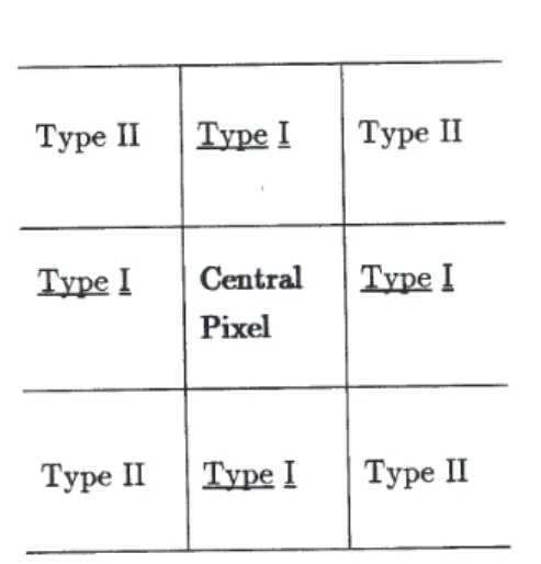
PRIOR STRUCTURE: MARKOV RANDOM FIELD HYPOTHESIS
A convenient way of representing a spatial structure of neighbourhood dependence probabilistically is to model the field as a Markov Random Field (MRF) which is the spatial equivalent of an autoregressive process. Having defined a certain number of types of neighbours which are constrained by the condition that they should form cliques (Chandler et
al., 1997), it is possible to estimate the ratio of the probability
of a pixel being wet (Xi =1) to its being dry (Xi =0). This is in terms of a number of parameters equal to the number of neighbour types plus one. Data analysis suggested that the neighbourhood structure illustrated in Fig. 1 would provide a simple and adequate representation of the spatial structure. There are two neighbour types and the Hammersley-Clifford theorem (Besag, 1986) yields:
Pr{Xi =1|rest of the field} /Pr{Xi =0|rest of the field} = exp {α+ β1A1 + β2A2} (2) where α, β1 and β2 are parameters, and A1 and A2 are the number of type 1 and 2 pixels which are wet.
FIRST TYPE OF EVIDENCE: DISAGGREGATED FIELD AT THE PREVIOUS TIME-STEP
The simplest way of representing the dependence between two consecutive time-steps is by using conditional probabilities of the state of a pixel at one time-step given its state at another. Note that because of the way the evidence is used in (1), these conditional probabilities are expressed in the following form:
p(yi,xi) = Pr{ Xi (t-1) =yi | Xi (t) = xi } (3) and thus two such probabilities are required, p(1,0) and p(1,1) .
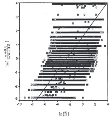
SECOND TYPE OF EVIDENCE: LARGE-SCALE RAINFALL INTENSITIES
A relationship between average real intensity and coverage over a grid-square is required. There are many studies identifying links between these variables (Eltahir and Bras, 1993; Onof et al., 1998). Here, however, a relationship is required that can be used in a distributional fashion, e.g. such that the residuals are approximately normally distributed (with mean 0). Data analysis suggests that this condition is fulfilled by the following relationship:
ln{ (w+0.5)/(n-w+0.5)} = a ln{R} + b + Z (4) where w is the number of wet pixels out of the n pixels in the grid square, R the average rainfall over it, a and b model parameters and Z a N(0, s2) distributed variable. This is
illustrated by a plot of the left hand side of (4) against ln{R} in Fig. 2.
N.G. Mackay, R.E. Chandler, C. Onof and H.S. Wheater
INTEGRATION OF THIS INFORMATION BY A RASTER-LIKE UPDATING OF THE FIELD
The fact that this information is available in conditional form means that the updating of the rainfall field according to Bayes’s theorem is best carried out as an updating of the value (0 or 1) of each pixel conditional upon its neighbours. Since the distribution of Z in (4) is a continuous one, the updating of each pixel takes the form of a sampling procedure according to a conditional posterior density function. Thus, at each pixel, this is calculated as a product of the conditional probability of the pixel’s state at the previous time-step, the conditional density function of the resulting coverage and the prior probability given from the log odds ratio in (1). The process is carried out at each pixel and repeated over the whole picture a large number (e.g. 100) of times. This is an implementation of the Gibbs sampler (Besag, 1986), and provides a field in which the state of a pixel is approximately distributed according to the posterior distribution of Xi.
IMPLEMENTATION
As mentioned above, the requirement of the knowledge of the previous disaggregated time-step entails that the algorithm is best started with a dry rainfall field. At each time-step, the iterative procedure of updating each pixel is initialised by starting with the disaggregated rainfall field from the previous time-step and the 100 iterations of the Gibbs sampler can then be carried out. At the edges, pixels
have fewer neighbours; the conditional probabilities are therefore scaled accordingly.
Rainfall intensities
This task can be subdivided into two parts:
l find a number of pixel intensities equal to the number of wet pixels by sampling from the marginal distribution of pixel intensity;
l choose to which pixel each sampled intensity is to be allocated.
MARGINAL DISTRIBUTION OF PIXEL INTENSITY
Many authors report that point rainfall intensities are approximately gamma distributed (Collier et al., 1992). Matsubyashi et al. (1984) find that for small areas of a few square kilometres, mean areal intensities are gamma distributed, with the distribution converging towards a normal distribution as the size of the area increases. This is not always the case (Oh, 1993), but for the scales of 4 km × 4 km or 8 km × 8 km, the rainfall intensities in the Arkansas data are found to be gamma distributed.
However, this information is not sufficient to sample the intensities in the disaggregation scheme because of the constraint that the average of the intensities over all the pixels should be equal to the grid-square intensity. The distribution of k independent gamma distributed variables with shape parameter υ and scale parameter η which are constrained by their sum kR is a beta distribution (Johnk, 1964) characterised by the following density function:
f X|kR (x) = 1/[ kR B(υ,(k-1)υ) ] (x /(kR))υ-1
(1 - x/(kR))(k-1)υ-1 (5)
where B(x,y) = Γ(x)G(y)/G(x+y) is the beta function (and
Γ the gamma function). Notice that the scale parameter of the gamma distribution does not appear, which is intuitively reasonable since all the scale information about the value of the pixel intensity X is governed by the sum kR so that a single parameter is required here.
The validity of this beta distribution assumption can be verified in the following way: for the July 1994 data, pixel intensities are normalised so that each grid-square has the same mean. The cumulative distribution of the pixel intensities is then plotted against the theoretical beta cumulative distribution with the same mean and standard deviation as the data. Figure 3 shows that this distribution does indeed provide a good fit and a Kolmogorov-Smirnov test at the 99% level does not reject the hypothesis of goodness of fit.
INTENSITY ALLOCATION
Data analysis of the July 1994 data is carried out to identify a simple feature of the spatial structure of the rainfall intensities. The intensities of all pixels and distances to the nearest dry pixel are ranked from the lowest to the highest, over the wet area the pixel belongs to. The distance used is the L1 or Manhattan metric illustrated in Fig. 4. Figure 5 is
a plot of the intensity ranking against the distance ranking (circles refer to any number of pixels less than 100 while a petal represents 100 pixels). It shows that higher intensities tend to occur at points which are further from the dry area.
This is confirmed by a Spearman correlation test yielding a correlation of 0.47 which is significant at the 99% confidence level.
This suggests the following intensity allocation scheme: 1. For each pixel, the L1 distance to the neighbouring dry
area is calculated.
2. This distance d is raised to the power p.
3. Pixels are then randomly allocated the sampled intensities, starting from the highest intensity, with a probability proportional to dp.
The power p which is empirically found to produce the best intensity field structure is p=5, so that the dependence upon the distance is highly non-linear.
Parameter estimation
Parameters are estimated for the period from July 1994 to June 1995. The parameters used for the MRF model and the dependence of areal intensity upon coverage are estimated by maximum likelihood while the temporal dependence probabilities are estimated by the corresponding frequencies in the data set.
A parameter set is estimated for each month to represent seasonality in the following way:
1. A set of parameters is calculated for each time-step in the period.
2. A weighted average of parameters over the month is then obtained using weights proportional to the conditional mean rainfall intensity (i.e. mean intensity over wet grid-squares) so that these averages are dominated by intensive rainfall events.
Fig. 4. Illustration of distance from edge calculated by L1 metric: wet areas are numbered with the value of their distance to the edge
of the rainfall field.
Fig. 3. Comparison of cumulative beta and data distributions Fig. 5. Rank of the pixel intensity against rank of pixel distance from
N.G. Mackay, R.E. Chandler, C. Onof and H.S. Wheater
3. Moving averages of these monthly parameters are then calculated over the year using a window of length 3 with weights of 0.25, 0.5 and 0.25 respectively, so as to produce a smoothed parameter set.
Model assessment
Model assessment was carried out on a storm starting at 17:00 on 14 July 1995 and finishing at 07:00 on 15 July 1995.
WET/DRY MODEL Correctly classified pixels
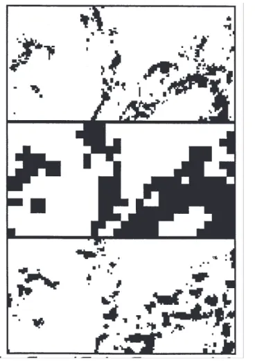
Figure 6 shows a black and white (wet/dry) example of a model realisation (top) compared with the data (bottom) at the fine-scale for 22:00; the coarse-scale picture used in the disaggregation is in the middle. The reconstruction is good in that 65.2% of the pixels within wet grid-squares have been classified correctly; however, there is some diagonal banding in the data that is not well reproduced.
The mean and variance over 100 realisations of the proportions of the correctly classified wet grid-squares are shown in Fig. 7 for each hour of the event: in general, the model classifies about 65 to 70% of the pixels correctly.
Coverage
The proportion of correctly classified pixels can however be well reproduced by a totally dry or wet field. Therefore, we must also look at a measure which is most important to the success of this scheme in terms of producing hydrologically realistic rainfall, i.e. the rainfall coverage. Figure 8 shows the coverage errors for the duration of the test storm. The quantities plotted are the mean over 100 realisations of the mean and variance over all grid-squares of the rainfall field of the difference between the true coverage of these squares and the modelled coverage. This demonstrates the ability of the scheme in reproducing coverages, since the mean error is mostly smaller than 4% or 1 pixel per grid-square, and the standard deviation less than 8%.
Fig. 6. Sample model output for wet area prediction Fig. 7. Modelled wet grid square coverage errors Fig. 8. Success rate for wet/dry pixel classification
Intensity scheme
To estimate the errors of this scheme independently of the success of the wet/dry algorithm, the intensity scheme is applied to the true wet/dry field.
To assess the goodness-of-fit quantitatively, the Mean Square Error (MSE) is used:
MSE = E [ S (xi - yi)2 ]
where X=xi and Y=yi are the modelled and observed pixel intensities respectively, k the number of wet pixels in a grid-square and the expectation is over all grid-grid-squares and over all realisations. By expanding:
MΣE = E [var[X] + var[Y] - 2 E {corr[X,Y]
var[X]var[Y] }] (6)
where the variance (var) and correlation (corr) are sample statistics taken over the pixels contained in a grid-square.
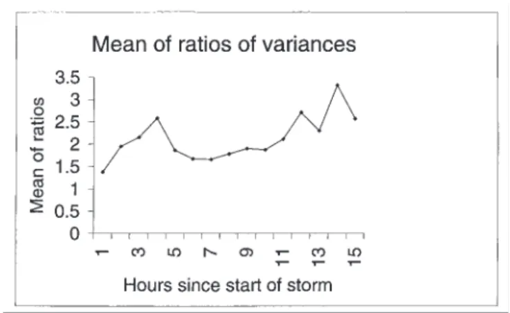
The terms in MΣE are examined in turn using 100 realisations of the disaggregated field. Figure 10 shows the mean over all grid-squares and all realisations of the ratio
THE WHOLE DISAGGREGATION SCHEME
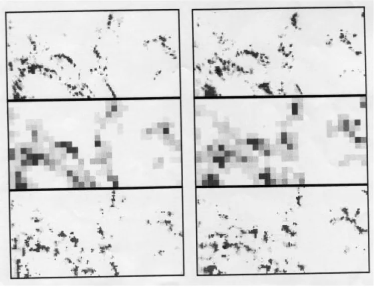
The performance of the whole disaggregation scheme can be assessed visually by looking at a sequence of model realisations from the storm of 14 July 1995 for two consecutive hours (22:00 and 23:00) compared to the observed data (Fig. 9a, 9b, shown overleaf).
Quantitatively, the variables examined for the intensity scheme in Figs. 10 and 11 are now plotted for the whole scheme in Figs. 12 and 13 respectively. The ratio of the
within-square variances has deteriorated only slightly
compared with the intensities-only case. This reflects the accuracy of the model at reproducing rainfall coverages. On the other hand, the intensity correlations between modelled and observed data are much smaller. This is largely due to the stochastic nature of the model which, for instance, correctly classifies only 65 to 70% of the pixels in the wet/ dry scheme. This measure is therefore of little use as an indicator of the appropriateness of the scheme as a whole.
Fig. 10. Variance of within wet grid-square intensities (intensity
model only)
of the within-square intensity variance for the observed data to that for the modelled data, i.e. of var[X]/var[Y]. There is, on average, one and a half to two times as much variance in the observed data as in the disaggregated image. Note that under the assumption of perfect correlation between observed and modelled data, MSE is minimal when the variances are equal.
Figure 11 shows the mean of the within-square intensity correlation between the observed and modelled data, corr[X,Y]. Fairly high correlations of 0.6 are achieved, which is encouraging, considering the simplicity of the intensity scheme in its present form.
Fig. 11. Correlation of within wet grid-square intensities (intensity
model only)
N.G. Mackay, R.E. Chandler, C. Onof and H.S. Wheater
Fig. 9. Model output for full algorithm (a and b: 14/7/95 at 22:00 and 23:00) with for each: the observed field at pixel resolution at the top,
the aggregated observed field in the middle and the modelled disaggregated field at the bottom.
Fig. 13. Correlation of within wet grid-square intensities
Conclusions and further work
A general modelling procedure has been developed for rainfall disaggregation which retains spatial and temporal memory and therefore has clear advantages over schemes generally available at present. The different components of the scheme have been assessed and found to be individually reasonable for the production of stochastic realisations of disaggregated rainfall fields. The overall model has also been shown to reproduce properties of the rainfall field with a reasonable degree of accuracy. This algorithm is expected to be of use either in providing greater detail to the rainfall forecasts obtained with meteorological models or as input to hydrological models which incorporate representations of the exchange of energy and water vapour and the
generation of runoff, since spatial and temporal memory are important factors in predicting response.
There remains a number of issues to address:
(1) Improvement of the intensity sampling and allocation scheme: another Markov Random Field approach is being considered to provide a more satisfactory representation of the spatial structure of the intensity distribution.
(2) Parameter estimation: at present, parameters are scale and site specific, which means that a large amount of data analysis is required for their estimation. A systematic examination of the variation of parameters from site to site and over different scales as a function of climatological characteristics is required.
(3) Model assessment: the performance of models such as these is difficult to assess in a formal manner. It would seem that an examination of their performance in conjunction with hydrological models is the proper approach to this problem.
References
Abourgila, A.E., 1992. Large-scale hydrological modelling of the
Nile basin, Unpubl. MSc thesis, Dept. of Civil and Environ.
Engin., Imperial College, London
Besag, J.E., 1986. On the statistical analysis of dirty pictures, J.
Roy. Stat. Soc., Series B, 48, 259–302
Brown, R., 1998. Personal communication, Met. Office, UK. Chandler, R.E., Mackay, N.G., Wheater, H.S. and Onof, C., 1997.
Bayesian image analysis and the disaggregation of rainfall,
Research Report No. 184, [http://www.ucl.ac.uk/stats/research/ abs97.html#184], Dept. of Statistical Science, University College London.
Collier, C.G., 1992. The application of a continental-scale radar database to hydrological process parameterization within General Circulation Models, J. Hydrol., 142, 301–18. Department of the Environment, 1996. Review of the potential
effects of climate change in the United Kingdom, 2nd Report,
HMSO, March.
Eagleson, P.S., 1978. Climate, soil and vegetation, 2. The distribution of annual precipitation derived from storm sequences, Water Resour. Res., 14, 713–21.
Eltahir, E.A.B. and Bras, R.L., 1993. Estimation of the fractional coverage of rainfall in climate models, J. Climate, 6, 639–644. Gregory, D. and Smith, R.N.B., 1990. Unified model
documentation paper 25: canopy surface and soil hydrology, Version 1. Technical report, Meteorological Office, Bracknell,
UK.
Johnk, M.D., 1964. Erzeugung von Betaverteilten und Gammaverteilten Zufallszahlen, Metrika, 8, 5–15.
Kedem, B., Chiu, L.S. and Karni, S., 1990. An analysis of the threshold method for measuring area-average rainfall, J. Appl.
Meteorol., 29, 3–20.
Matsubayashi, U., Takagi, F. and Tonomura, A., 1984. The probability density function of areal average rainfall, J.
Hydrosci. Hydraul. Eng., 2, 63–71.
Molders, N., Raabe, A. and Tetzlaff, G., 1996. A comparison of two strategies on land surface heterogeneity used in a mesoscale-meteorological model, Tellus, 48A, 733–749.
Oh, L., 1993. Analysis of rainfall disaggregation in GCMs, Unpubl. MSc Thesis, Dept. of Civil and Environ. Engin., Imperial College, London.
Onof, C. and Wheater, H.S., 1996a. Analysis of the spatial coverage of British rainfall fields, J. Hydrol., 176, 97–113. Onof, C. and Wheater, H.S., 1996b. Modelling of the time series
of spatial coverages of British rainfall fields, J. Hydrol., 176, 115-31.
Onof, C., Mackay, N.G., Oh, L. and Wheater, H.S., 1998. An improved disaggregation technique for GCMs. J. Geophys. Res.,
103, 19577–19586.
Rowntree, P.R., 1988. Land surface parameterizations. In: Proc.
of ECMUF workshop on parameterization of fluxes over land surfaces, Meteorological Office, Bracknell, UK.
Seth, A., Giorgi, F. and Dickinson, R.E., 1994. Simulating fluxes from heterogeneous land surfaces: explicit sub-grid method employing the biosphere-atmosphere transfer scheme (BATS),
J. Geophys. Res., 99, 18,651–18,667.
Sivapalan, M. and Woods, R.A., 1995. Evaluation of the effects of general circulation models subgrid variablity and patchiness of rainfall and soil moisture on land surface water balance fluxes. In: Scale Issues in Hydrological Modelling, J.D. Kalma and M. Sivapalan, (Eds.), Wiley, Chichester, UK. 453–473.
Steiner, M., Smith, J.A., Burges, S.J., Alonso, C.V. and Darden, R.W., 1998. Extremes of spatial gradients in rainfall accumulations, Sixth International Conference on Precipitation:
Predictability of rainfall at the various scales, Hawaii.
von Storch, H., Zorita, E. and Cubasch, U., 1993. Downscaling of global climate change estimates to regional scales: an application to Iberian rainfall in winter-time, J. Climate, 1161–1171. Warrilow, D.A., Sangster, A.B. and Slingo, A., 1986. Modelling
of land surface processes and the influence on the European Climate, Technical Report CDTN38, Meteorological Office,
Bracknell , UK.
Wheater, H.S., Jolley, T.J., Onof, C., Mackay, N. and Chandler, R.E., 1999. Analysis of aggregation and disaggregation effects for grid-based hydrological models and the development of improved precipitation disaggregation procedures for GCMs,