The demand for school meal services by
Swiss households
M. Filippini
G. Masiero
yD. Medici
zPublished in Annals of Public and Cooperative Economics (2014), 85(3): 475-495 http://onlinelibrary.wiley.com/journal/10.1111/(ISSN)1467-8292
Abstract
In this paper we investigate the household demand for childcare during lunchtime at school using a stated preferences approach. Data are collected through phone-structured interviews to 905 residents with children in the German-speaking region of Switzerland during 2007. Poisson models with random and …xed e¤ects are used to ex-plore factors a¤ecting the demand. Ordinal probit models are also considered as an alternative to count data models. The results show that price, household income, satisfaction with the current childcare service, family composition, and the area of residence signi…cantly af-fect the number of weekly services demanded. We estimate that the willingness to pay for childcare during lunchtime is between 7.90 and 11.70 Swiss francs per day and does not depend on household income. Keywords: Childcare service, school meal service, panel count data, Poisson regression, willingness to pay, ordinal probit model.
JEL classi…cation: D12, H31, H42, J13
Department of Economics, University of Lugano and ETH Zurich, Switzerland.
yDepartment of Engineering, University of Bergamo, Italy and Department of
Eco-nomics, University of Lugano, Switzerland. Corresponding author. E-mail:
[email protected]. The empirical analysis reported in this paper exploits a dataset built for a project commissioned to the Institute of Economics at the University of Lugano and …nanced by four Swiss cantons (Aargau, Basel-City, Basel-Land and Solothurn).
1
Introduction
In most OECD countries, parents face considerable challenges when trying to reconcile their family and work commitments, since all-day childcare fa-cilities are not always available (OECD 2007). Parents who decide to work full-time or part-time may pay a substantial amount for private childcare services. Other parents prefer to stay out of the job market and provide full-time care directly to their children. Problems with the organization of care before and after school hours and during lunchtime are substantial, particularly for families with children at primary school. Supervised school meals service and extracurricular activities may improve household choices and are probably bene…cial to those parents who give value to opportunities at work.
The analysis of household preferences and willingness to pay for school meal and childcare services may represent an important step towards poli-cies aiming at improving reconciliation between family and work life. In Switzerland, municipalities are mainly responsible for the decision to o¤er
supervised school meal services.1 Since cantonal (state) authorities usually
play a secondary role in this decision process, the supply of childcare during lunchtime and school meal services is rather heterogeneous across and within
cantons.2 In several cantons, most of the municipalities do not supply
su-pervised school meal services but many of them have recently discussed the possibility to increase the supply. Local governments can provide a childcare and meal services during lunchtime, between morning classes and afternoon
1Usually, school time is organized in two periods: morning classes (8.30 a.m. - 11.30
a.m.) and afternoon classes (1.30 p.m. - 4 p.m.). During the lunchtime break children can have their lunch, play and rest if a school service is available, or alternatively go home.
2Switzerland is a federal State with a largely decentralized education system. Primary
school education is mandatory and generally supplied by the State. The tasks of the education system are shared between three levels of government - the Confederation, the cantons and the municipalities - which work together in their respective areas of responsibility to ensure high quality in education. The organization and the regulation of the education system is not homogeneous across the territory, since each of the 26 cantons has its own subsystem of primary schools. The cantons and their municipalities
are responsible for the organization and …nancing of primary schools. In particular,
municipalities assume competences on pre-school, primary and lower secondary levels.
classes. When a supervised school meal service is not available, parents look after their children between morning and afternoon classes or use some infor-mal care mode provided by relatives, neighbours or friends. Moreover, those municipalities already providing school meal services usually set a relatively low price, which is unsatisfactory because it does not cover the average cost of the service. This pricing policy has led to …nancial problems. Conse-quently, municipalities that are interested in providing childcare and school meal services are also interested in learning more about the willingness to pay of households.
In this paper, we investigate the demand for school meals and childcare during lunchtime at primary schools in Swiss cantons characterized by a lack of supply of supervised school meal services. We consider four cantons which are representative of the northwest part of Switzerland. These cantons and their municipalities are about improving the supply of childcare services at primary school, by introducing a supervised meal service available between the end of the morning classes and the beginning of the afternoon classes. Using a stated preferences approach, we analyse the hypothetical weekly demand of school meals and childcare, conditional on household and service characteristics. First, we collect data on the weekly demand of school meals and childcare by 905 households. We then apply count data models to study factors a¤ecting household preferences. Ordinal probit models are also considered as an alternative to count data models. Finally, we assess the willingness to pay for the new service and discuss improvements in the pricing policy for an e¢ cient provision of school meal and childcare services. The literature lacks empirical studies on the demand for supervised school meals. Some studies vaguely relate to our analysis, although their focus is on the demand for di¤erent types of diet rather than the demand for meals. Lee (1987) investigates the demand for varied diet in US house-holds between 1977 and 1978. Count data approaches, such as the Poisson model and the negative binomial model, are used to examine the impact of household characteristics on the number of di¤erent food items consumed during a week. The results show that an increase in food expenditure
creases the number of food items consumed at home. Moreover, the number of food items consumed at home is positively related to the number of house-hold members. Akin et al. (1983) analyse participation in the US National School Lunch Program by 1222 children. Following the traditional utility theory, the authors write the demand for school meals as a function of the price of meals, the price of complements and substitutes, the budget con-straint and several socioeconomic characteristics. A vector of nutrient taste variables is added to the demand function. The demand is estimated by means of ordered probit models where the dependent variable is the quan-tity of school meals. Based on the estimates, a 50 percent increase in the full price of school lunches for students is expected to reduce the participation in the National Program by 20 percent. The authors a¢ rm that taste variables are important in assessing the demand for school meals. Park and Capps (1997) estimate the demand for prepared meals by US households using the 1987-1988 Nationwide Food Consumption Survey and applying a Heckman two-stage procedure. Prepared meals are de…ned as those ready to eat and to cook. Households with younger, more educated and time-constrained man-agers are more likely to purchase prepared meals. Income elasticities range from 0.07 to 0.13, while own-price elasticities range from -0.23 to -0.66. The presence of teenagers in a household is positively associated with expen-ditures of prepared meals. Moon et al. (2002) identify socioeconomic and demographic factors a¤ecting the demand for varied diet as measured by the count of food items and the Entropy index. The authors use data collected in Bulgaria in 1997. Consumer preferences for food variety exhibit di¤erent patterns depending on the length of time allowed for consumption. Daily variety deviates from weekly and monthly variety and regional e¤ects di¤er across periods. Finally, some studies focus on health problems related to school lunches. Schanzenbach (2009), for instance, investigates the e¤ects of participation in the National School Lunch Program. Although initial rates of obesity are similar among participants and non-participants, the rate of obesity among participants is higher after some time.
Through this paper, we provide a …rst empirical analysis of the demand
for meal and childcare services at primary school in Switzerland. Our analy-sis allows to disentangle factors a¤ecting household choices and to calculate the willingness to pay for meal and childcare services at school. We believe this represents an original contribution to the modest economic literature on the demand for school meal services.
The remainder of the article is structured as follows. In Section 2, we specify a model of the demand for supervised school meals. Section 3 is de-voted to the survey design and data description. In Section 4 and Section 5, we present the estimation results of our model and calculate the willingness to pay for supervised school meal services by Swiss households respectively. The use of ordinal probit models as an alternative to count data models is discussed in Section 6. Concluding remarks and policy considerations are discussed in Section 7.
2
Model speci…cation
Family decisions regarding the demand for school meal and childcare services depend upon several factors, primarily job opportunities and constraints, and preferences for family life. The analysis of the relationship between household choices in the labour market and the demand for school services is beyond the scope of this paper. Instead, we focus on the demand for supervised school meals consequently to household decisions in the labour market, and try to disentangle how di¤erent family characteristics are related to this demand. Hence, we hypothesize that the household demand for school meal and childcare services is generated by the following function:
Q = f (z), (1)
where Q is the hypothetical number of supervised meals per week and z is a vector of k socioeconomic variables, including household income, and meals price.
To specify an econometric model, it is worth noticing that the dependent variable in the above equation (1) is a count variable that indicates the num-ber of times parents buy supervised school meal services for their children
within a week. Linear regression models are not suitable for count outcomes since the estimation results can be ine¢ cient and biased. Models that specif-ically account for the generation process of the data are more suitable for count outcomes. In the literature, we …nd two main econometric approaches: the Poisson regression and the negative binomial regression. Some authors (Akin et al., 1983) also use ordered logit or probit models. However, the econometric literature (Greene, 2003; Cameron and Trivedi, 2005) advises
count models as the most appropriate approach.3 Finally, count models o¤er
the advantage that the calculation of consumer surplus is relatively simple. Several studies apply count models to explore, for instance, the demand for hospitalizations, the number of beverages, the number of visits to a national park, or the number of patents. Cameron and Trivedi (1986) analyse factors a¤ecting the frequency of doctors consultations, Mullahy (1986) explores factors that in‡uence the number of beverages, and Carpio et al. (2008) investigate the demand for agritourism in the United States.
To estimate the demand model, we …rst consider a Poisson regression. Unobserved heterogeneity that remains constant over time is taken into ac-count by means of random e¤ects (RE) and a …xed e¤ects (FE) versions
of the Poisson panel regression.4 Our model includes several time-invariant
covariates and one time-variant variable, the price. For this reason, the esti-mation results obtained with the …xed e¤ects version are not very interest-ing. For comparison purposes with the Poisson regression, we also estimate the demand model using a negative binomial regression. The possibility of applying a two-part model and a zero-in‡ated count model has also been discussed. However, due to the fact that the zeros and the positive values in our sample come from the same generation process (see Section 3), these econometric approaches are not advisable (Cameron and Trivedi, 2005).
To focus on the Poisson model, we recall that the Poisson probability
3For the purpose of comparison we also estimate ordered models and report the results
in Section 6.
4See Hausman et al. (1984), Cameron and Trivedi (1998), Greene (2003) and Baltagi
(2008) for details on Poisson regressions for panel data.
density function can be written as:
P (Q = q) = e
q
q! , (2)
where q = 0; 1; 2; ::: is a random variable indicating the number of times an
event occurs, and is the parameter of the Poisson distribution. Precisely,
is the expected number of times an event occurs within a given time. This is a one-parameter distribution with both the mean and the variance of Q equal to .
In our case, the Poisson distribution de…ned by (2) assumes that all families have the same expected demand in terms of the number of school meal and childcare services. Since this assumption may not be very realistic,
we can allow for heterogeneity in by using the following Poisson regression
model:
i = exp(zi ), (3)
where i is a function of vector of socioeconomic characteristics of the
house-hold and price for the service (zik). The subscript i indicates the household
and are parameters. Taking the exponential of zi forces the expected
count to be positive, which is required by the Poisson distribution.
Socioeconomic control variables (zk) provide information on the price for
meal service (Price), the household monthly income (Income), the structure of the family in terms of number of members and their age, the level of education, work constraints and the area of residence of the households, and satisfaction with the current care mode. More precisely, we include dummy variables to capture whether the child is cared by non-family members (Care
by others),5 whether the family lives in urban or rural area (Urban), and the
canton of residence (AG, BL, BS, or SO). We also include a dummy to indicate if the respondent is the child’s mother (Mother ), whether or not
5Parents can ask relatives, neighbours or friends to look after their children during
lunchtime. This type of childcare is usually unpaid.
V ariable Desc rip tion Price Price for the servi ce (in S wiss fra n cs ) Inc ome Hous ehold mon thly inc o m e (in cat ego ries of 2000 Sw is s fr an cs: 0-2000, 2001 -40 00, ... , 1 0001-12000, a b o v e 12000) up to 6000 Hous eh o ld mon th ly inc ome b elo w 6001 Swiss franc s (u p to 6000= 1; 0 othe rwise ) b et w ee n 6001 and 8000 Hous eh o ld mon th ly inc ome b et w een 6 001 an d 8000 S wi ss fr an cs (b et w een 6 001 an d 8000= 1; 0 othe rwis e) ab o v e 80 00 Hous eh o ld mon th ly inc ome ab o v e 8000 Swiss franc s (ab o v e 80 00=1; 0 ot h erwise) Price x In come In ter ac tion b et w een price a n d in come Car e b y o th ers Th e child is car ed b y p eop le other th a n the paren ts (Car e b y o th ers=1 ; 0 o th erwi se) BL Th e fa m ily li v es in can ton Base l-Co u n try (BL= 1; 0 othe rwise ) BS Th e fa m ily li v es in can ton Base l-Ci ty (BS = 1; 0 othe rwise ) A G Th e fa m ily li v es in can ton Aar gau (A G= 1; 0 oth er w is e) SO Th e fa m ily li v es in can ton Solot h u rn (SO= 1; 0 othe rwise ) Ur b an Ur b an region (Urban=1; 0 otherwise) Moth er Th e resp o n de n t is th e m o th er (Mothe r=1; 0 ot h erwi se) Age Age of the re sp on den t Nat ionalit y Th e resp o n de n t is Swiss (N ationali ty=1; 0 ot h erwi se) W ork W ork in g rate o f the resp on den t (in p er cen ta ge ) Univ ersit y Th e resp o n de n t h as a u niv ersit y degree (U n iv er si ty =1; 0 ot h erwise) Satisf a cti on P ar en ts a re sati s… ed with curr en t ca re mo d e (S at isf actio n =1 ; 0 oth er w is e) Child a ge Age of the ch ild con sidered in th e su rv ey Num b er of ch ildren b el o w 3 y ear s Num b er of additional ch il d re n y oun ger than 3 b et w ee n 3 an d 5 Num b er of additional ch il d re n b et w ee n 3 a n d 5 y ear s of a ge b et w ee n 6 an d 10 Num b er of additional ch il d re n b et w ee n 6 a n d 1 0 y ear s of age b et w ee n 11 an d 15 Num b er of additional ch il d re n b et w ee n 11 an d 15 y ear s of age Adu lts M o re th an tw o adu lts o ld er than 1 5 (Ad ults= 1; 0 oth er w is e) P a ren ts Both par en ts li v e in the hou seh ol d (P aren ts=1; 0 o th erwi se) T a b le 1 : L is t o f v a ri a b le s a n d d es cr ip ti o n .
the respondent is a foreigner (Nationality), and has a university degree (Uni-versity). Other covariates includes the age of the respondent (Age) and the percentage of work of the respondent (Work ). In addition, we consider household satisfaction with the current care mode (Satisfaction) and the age of the child (Child age). If the family has more than one child, the number of additional children is measured by covariates for di¤erent age categories (below 3 years of age, between 3 and 5, between 6 and 10, and between 11 and 15 ). A dummy variable (Adults) indicates whether there are more than two adults in the household, i.e. people older than 15. Finally, we consider whether or not both parents live in the household (Parents). Socioeconomic variables are listed and described in Table 1.
Given equations (2) and (3) and the assumption that the events are independent, it is straightforward to estimate our Poisson regression para-meters ( ) by means of a maximum likelihood procedure. The log-likelihood function for the Poisson regression model is given by:
L( ) =
N
X
i=1
[qi(zi ) exp(zi ) ln qi!], (4)
where N is the number of observed values qi in the sample.
In our model speci…cation, the parameter estimates (^) indicate the im-pacts of the kth-independent variable on the number of school meal and childcare services demanded. The signs of the estimated parameters indi-cate the direction of the impacts. These parameter estimates can be used
in several ways.6 In this study, we mainly use the results to compute the
percentage change in the expected count for a -unit change in one of the ex-planatory variables, for instance a socioeconomic characteristic of the
house-hold (zk), holding all the other variables constant. This can be computed
as:
= 100 [exp( k ) 1]. (5)
Consequently, we will discuss the impact of changes in the socioeconomic
6See Long and Freese (2003) for a discussion on this issue.
characteristics of households in terms of percentage change in the number of school meal and childcare services households are willing to purchase.
3
Survey design and data
To investigate the demand for supervised school meals, we adopt a stated preferences approach, i.e. we use data from hypothetical markets. This approach is driven by the limited number of municipalities currently o¤ering supervised school meals within the country. Since families living in cantons considered in our analysis do not have the possibility to purchase supervised school meal services, their demand is not revealed.
Data were collected through phone-structured interviews administered to households with children at primary schools and living in one of the four cantons of the northwest part of Switzerland, a German-speaking region. The survey was conducted during November 2007 and a speci…c software helped to input the answers. The average length of an interview was about 17 minutes. The data set obtained for the analysis was part of a project commissioned to the Institute of Economics at the University of Lugano and …nanced by four Swiss cantons (Aargau, Basel-City, Basel-Land and Solothurn).
The interview was made of two parts. In the …rst part, we asked infor-mation on the demand for supervised school meal services. In the second part, we collected information on the socioeconomic characteristics of the households. Also, we collected information on the use of alternative care services when parents are unable to directly provide care to their children. At the beginning of the interview, the characteristics of a typical supervised
school meal service were presented to the household.7
During 2007-2008, primary schools in our regions were attended by 63155 pupils, 32150 of which were boys (50.9%) and 31005 girls (49.1%). Foreign
7The school meal and childcare services start at the end of the morning classes and
conclude at the beginning of the afternoon classes. During this period, children can have their lunch, play, rest or to do homework. The sta¤ is trained to take care of children. The meal service is delivered within the school or in another building/facility nearby.
pupils represented 24.7% of the children population. There were 3166 classes in total, each of them with 20 children on average. Families received a letter to explain the characteristics of the study, and a coupon to ask for participa-tion. Around 60% of the respondent households (3645) agreed to answer the questionnaire in the form of a phone interview. However, because of budget
limitation, only 905 families were randomly selected for the interview.8 The
…nal sample was representative of the households population with children at primary school in each canton, as well as class level and children age.
Some descriptive statistics for the households sample are provided in Table 2. Households characteristics are grouped in two main categories: so-cioeconomic characteristics of households, and children characteristics and family composition. Note that the number of observations varies with house-holds characteristics since not all interviewed househouse-holds answered all the questions.
Concerning socioeconomic characteristics, households are initially clas-si…ed according to three monthly income classes: low, medium, and high. 32% of the sample (280 families) indicate a level of income below 6001 Swiss francs per month. 36% of families (320 households) gain between 6001 and 8000 Swiss francs per month. Finally, 32% of families (282 households) gain more than 8000 Swiss francs per month. Regarding the other socioeconomic characteristics, 83% of households live in urban areas and only 17% in rural areas. Households are equally distributed across the four cantons (25% in each canton). Mothers are responsible for the care of children in about 91%
of the cases, while fathers only in 9%.9 For this reason, the average level
of employment of the respondent is relatively low (38%), which corresponds roughly to two working days full-time per week. The average age of the respondent is 40 years. The respondents are Swiss in 83% of cases and have a university degree in about 13% of cases. As many as 47% of children are cared during lunchtime by people other than the parents, for instance
rela-8Given the population size, our number of respondents allows to obtain 95% con…dence
levels with 3% precision.
9Note also that the respondent to the questionnaire is the father in about 9% of cases.
Variable Obs. Mean/Frequency Std. Dev. Min Max
Price 1783 9.92 5.01 2.5 22.5
Socioeconomic characteristics of households
Income 882 4.13 1.34 1 7 up to 6000 280 31.75% between 6001 and 8000 320 36.28% above 8000 282 31.97% Age 905 40.47 5.50 21 88 Work 902 37.53 33.37 0 100 Care by others 905 47.18% BL 905 25.08% BS 905 25.08% AG 905 24.97% SO 905 24.86% Urban 905 83.09% Mother 904 90.93% Nationality 905 82.98% University 905 13.37% Satisfaction 905 51.27%
Children’s characteristics and family composition
Child age 905 9.25 2.72 5 15 Number children below 3 905 0.10 0.31 0 2 between 3 and 5 905 0.33 0.51 0 5 between 6 and 10 905 1.04 0.74 0 4 between 11 and 15 905 0.47 0.69 0 3 Adults 905 89.94% Parents 905 84.20%
Table 2: Descriptive statistics for the household sample (N=905). tives or neighbours. Only in 51% of the cases, parents are satis…ed with the current childcare mode during lunchtime.
Variables related to the family composition and children’s characteristics include the number of children and adults in the household as well as the age of the children. The average children age is about 9 years old. On average, households include 0.1 additional children younger than 3, and 0.33 addi-tional children between 3 and 5. On average, families have one addiaddi-tional child between 6 and 10 years old, and 0.47 additional children between 11 and 15 years old. In about 90% of households, there are more than two
adults (older than 15), and in 84% of households both parents live together. To collect information on the demand for supervised school meals, house-holds were asked to consider up to …ve levels of price for the meal and child-care services and to state the maximum number of services they would buy at each level of price. The other characteristics of the service, for instance the number of children per sta¤ member or the opening hours of the service, were not changed. The initial level of price was set according to household’s monthly income. Respondents were asked to consider their employment sta-tus as unchanged when answering the questions. Three initial levels of price were proposed to the respondents: 2.50 Swiss francs for low-income fami-lies, 7.50 Swiss francs for medium-income famifami-lies, and 12.50 Swiss francs for high-income families. To simulate the Swiss customary pricing policy, subsidized prices were proportional to household income. Thus, di¤erences in income between rural and urban areas were indirectly considered by hy-pothetical prices. The initial price was then increased by 2.50 Swiss francs, repeatedly, for each income group. The experiment stopped as soon as the respondent declared he/she was unwilling to buy any unit at the proposed level of price.
Clearly, the maximum number of services a household could buy was equal to …ve, i.e. the number of days the supervised meal service could be available within a week. Since some of the interviewed households were not interested in the supervised school meal service, they were not asked questions regarding the willingness to purchase school meal and childcare services during lunchtime according to di¤erent levels of price. Among the 905 households 679 (75.03%) provided information on the demand for su-pervised school meals (226 households were not interested in the service).
Frequencies of supervised school meals demanded at di¤erent levels of price for low-income, medium-income, and high-income households, are re-ported in Table 3. A total of 269 households (39.62%) declared they were not interested or not willing to purchase supervised school meals at the pro-posed initial price. This implies that around 60% of households were willing to buy at least one unit of service at the lowest proposed price. Generally,
L o w -income hous eholds 2.50 CHF 5 CHF 7.50 CHF 10 CHF 1 2.50 CHF T otal Quan tit y O b s. % O b s. % O b s. % O b s. % Obs. % Obs . % 0 85 14 .24 2 0. 34 3 4 5. 70 29 4.8 6 29 4.86 179 29.98 1 25 4. 19 31 5. 19 3 2 5. 36 27 4.5 2 10 1.68 125 20.94 2 42 7. 04 40 6. 70 3 1 5. 19 15 2.5 1 13 2.18 141 23.62 3 28 4. 69 28 4. 69 1 6 2. 68 11 1.8 4 3 0.50 86 14.41 4 8 1. 34 8 1. 34 3 0. 50 1 0.1 7 0 0.00 20 3.35 5 20 3. 35 14 2. 35 5 0. 67 4 0.6 7 3 0.50 46 7.71 T ot al 208 34.84 123 20.60 121 20.27 87 1 4.57 58 9. 72 59 7 100. 00 Mi d dl e-income hou seho lds 7.50 CHF 10 CHF 12.50 CHF 15 CHF 1 7.50 CHF T otal Quan tit y O b s. % O b s. % O b s. % O b s. % Obs. % Obs . % 0 100 16 .03 29 4. 65 56 8. 97 27 4. 33 16 2.56 228 36.54 1 43 6. 89 47 7. 53 29 4. 65 17 2. 72 13 2.08 149 23.88 2 66 10 .58 45 7. 21 22 3. 53 12 1. 92 6 0.96 151 24.20 3 27 4. 33 20 3. 21 9 1. 44 6 0. 96 3 0.48 65 10.42 4 5 0. 80 3 0. 48 3 0. 48 2 0. 32 0 0.00 13 2.08 5 9 1. 44 6 0. 96 2 0. 32 1 0. 16 0 0.00 18 2.88 T ot al 250 40.06 150 24.04 121 19.39 65 1 0.42 38 6. 09 624 100. 00 High-income hous eholds 12. 50 C H F 15 CHF 17.50 CHF 20 CHF 22.50 CHF T otal Quan tit y O b s. % O b s. % O b s. % O b s. % Obs. % Obs . % 0 84 14 .95 28 4. 98 5 1 9. 07 21 3.7 4 20 3.56 204 36.30 1 41 7. 30 41 7. 30 2 3 4. 09 19 3.3 8 8 1.42 132 23.49 2 60 10 .68 43 7. 65 1 9 3. 38 6 1.0 7 2 0.36 130 23.13 3 23 4. 09 14 2. 49 1 0 1. 78 7 1.2 5 3 0.53 57 10.14 4 6 1. 07 5 0. 89 4 0. 71 4 0.7 1 3 0.53 22 3.91 5 7 1. 25 6 1. 07 2 0. 36 1 0.1 8 1 0.18 17 3.02 T ot al 221 24.38 137 24.38 109 19.40 58 1 0.32 37 6. 58 56 2 100. 00 T a b le 3 : D em a n d fo r sc h o o l m ea ls b y p ri ce a n d h o u se h o ld in co m e. 14
we observe that for a given level of quantity, the number of households will-ing to buy decreases with an increase of income, which is in accordance with the law of demand for normal goods. Moreover, the number of house-holds demanding a certain quantity of meal and childcare services decreases when the price increases, ceteris paribus. On average, a low-income family would be willing to buy 1.56 supervised lunches during a week at the lowest proposed level of price (2.50 Swiss francs); a medium-income family would be willing to buy about 1.28 supervised lunches; and a high-income family would purchase 1.31 supervised lunches. The average price that households are willing to pay for a supervised school meal is reported in Table 2 and
corresponds to 9.92 Swiss francs.10
4
Estimation results
Count data models help us to identify the most important factors that in‡u-ence the number of school meal and childcare services demanded by house-holds during the week. We can now present the results from the estimation of count models used to analyse the hypothetical demand for supervised school meals: a Poisson regression, a negative binomial regression, and a Poisson regression with random e¤ects and …xed e¤ects (see Table 4). The results of a pooled Poisson regression and a pooled negative binomial re-gression are reported together for the purpose of comparison. These results are similar. The use of a negative binomial regression instead of a Poisson regression is indicated in presence of signi…cant overdispersion, i.e. when the variance exceeds the mean. We performed a simple overdispersion test
statistic (a formal test on the null hypothesis of equidispersion).11 The
re-ported t-statistic is asymptotically normal under the null hypothesis of no overdispersion. The coe¢ cient of our test is 0.089 and is highly signi…cant, which suggests that equidispersion cannot be rejected. Consequently, the
10This is obtained as the average price over families willing to purchase at least one
unit of the service. Perhaps if the hypothetical prices were lower, some households would be induced to purchase services, which would a¤ect the average.
11See Cameron and Trivedi (1990) for details.
V ariable P oisson N egat iv e binomial P oisson wit h RE P oisson wit h FE Co e¤ . S .E . Co e¤ . S.E. Co e¤ . S.E. Co e¤ . S .E. Cons tan t 0.637 0.2 35 0.651 0.2 58 0.6 44 0.40 4 Price -0.045 0.0 06 -0.045 0.0 07 -0. 085 0.00 7 -0.127 0.0 07 Inc ome 0.084 0.0 23 0.083 0.0 26 0. 184 0.03 6 Car e b y o th ers 0.037 0 .047 0.0 35 0.052 0.12 0 0.080 BL 0. 119 0.0 64 0.113 0. 069 0.17 9 0.10 4 BS 0.230 0.0 64 0.233 0.0 70 0.200 0.1 05 A G 0.11 2 0.0 66 0.107 0. 071 0 .083 0. 104 Ur b an 0.169 0.0 73 0.167 0.07 9 0.1 58 0.11 3 Moth er 0.039 0 .083 0.0 24 0.091 -0.064 0.140 Age 0.003 0 .004 0.0 03 0.005 0.002 0.007 Nat ionalit y -0.130 0.0 53 -0.128 0.05 9 -0.1 32 0.09 1 W ork 0.003 0.0 01 0.003 0.00 1 0.0 02 0.00 1 Univ ersit y 0.124 0.0 59 0.126 0.06 5 0.1 41 0.10 4 Satisf a cti on -0.281 0.0 45 -0.291 0.04 9 -0. 418 0.0 73 Child a ge 0.004 0 .015 0.0 04 0.016 0.015 0.025 Num b er chil d re n b elo w 3 -0.046 0 .067 -0.0 42 0.073 -0 .072 0.110 b et w een 3 an d 5 -0.148 0.0 54 -0.148 0.05 8 -0.1 25 0.08 7 b et w een 6 an d 10 -0.201 0.0 39 -0.197 0.04 2 -0.2 18 0.0 62 b et w een 11 and 15 -0.182 0.0 47 -0.180 0.05 1 -0. 196 0.0 74 Adu lts -0.121 0 .085 -0.1 11 0.095 -0.165 0.159 P a ren ts -0.242 0.0 77 -0.243 0.08 5 -0.245 0.1 39 Ps eud o R-s q u ar ed 0. 057 0.044 -Log-Li k el iho o d -2 666.30 -2657. 10 -2555. 83 -1214.31 Num b er of o b se rv atio n s 17 54 1754 1754 1 485 N o te : * , * * a n d * * * d e n o te st a ti st ic a l si g n i… c a n c e a t 1 0 % , 5 % a n d 1 % le v e ls . T a b le 4 : E st im a ti o n re su lt s o f re g re ss io n m o d el s fo r co u n t d a ta . 16
Poisson regression approach sounds appropriate. However, to take the un-observed heterogeneity that remains constant over time into account, we further estimate random e¤ects and …xed e¤ects versions of the Poisson
panel regression and report the results in the last columns of Table 4.12
Since we considered di¤erent initial levels of price according to household income, we also run Poisson regressions where we interact the price variable with the income variable. The goal of this model speci…cation is to analyse whether the willingness to pay for a supervised school meal depends upon income. The estimation results will be discussed later in Section 5 to assess the willingness to pay for school meal and childcare services. We also es-timate models separately for each income class. These estimations are not reported in the table since the main results are unchanged.
To brie‡y compare the Poisson regression and the negative binomial re-gressions along with the Poisson regression with random e¤ects, note that the signs of all the coe¢ cients are the same. Di¤erences are observed as with respect to the level of signi…cance. Generally, the coe¢ cients of the Poisson with random e¤ects are less signi…cant than the Poisson regression and the negative binomial regression. In particular, the area of residence, the na-tionality, the percentage of work, the level of education, and the number of additional children between 3 and 5 years old are not signi…cant anymore in the Poisson model with random e¤ects.
To discuss the sign and the level of signi…cance of the estimated parame-ters in more details, we can start by the price of the service. As expected, the coe¢ cient of price is negative and highly signi…cant. Higher levels of price would clearly decrease the number of supervised school meals demanded by households.
Focusing on children’s characteristics and family composition, we observe
12The Hausman test on a reduced form of the model (only with time-invariant
vari-ables) suggests the use of …xed e¤ects. However, as pointed out by Cameron and Trivedi (2005), an important limitation of the …xed e¤ects approach is that the coe¢ cients of the explanatory variables are “very imprecise”if variation over time is dominated by variation across respondents (between variation). See also Clark and Linzer (2012) for a discussion about the use of …xed e¤ects and random e¤ects. Moreover, as discussed before, the number of explanatory variables in the …xed e¤ects version is limited to one.
that three covariates are highly signi…cant: the number of children between 6 and 10 years old, the number of children between 11 and 15, and the pres-ence of both parents in the household (only in the Poisson and the negative binomial regressions). The impact of these covariates on the number of ser-vices demanded is negative. Hence, the presence of additional children and the presence of both parents decrease the number of school meal and child-care services demanded. This could be explained by the fact that parents with more children are more likely to look after their children directly and prepare meals at home. Also, the number of additional children younger than 3 and the number of additional children between 3 and 5 reduce the number of services demanded. However, the former variable is never sig-ni…cant, and the latter variable is highly signi…cant in the Poisson and the negative binomial regressions. Similarly, the presence of children older than 15 is not signi…cant. Finally, child’s age has a positive impact on the number of school meal and childcare services demanded, although the e¤ect is not signi…cant.
Regarding socioeconomic factors, the e¤ect of household income is pos-itive and highly signi…cant. As expected, a higher income is associated to an increasing number of services demanded. The level of education of the respondent and the area of residence have also a positive impact on the num-ber of school meal and childcare services, although this impact is not highly signi…cant in the Poisson regression with random e¤ects. The age of the respondent is always poorly signi…cant. Conversely, the canton of residence in the case of Basel-City and Basel-Country has a positive impact and is signi…cant at less than 10% in the Poisson regression with random e¤ects. This impact is measured with respect to the reference canton of Solothurn
Finally, we consider the level of satisfaction with the current care service. This indicator is related to childcare services currently used by households when children are not at school. Satisfaction with other care services has a negative and highly signi…cant impact on the number of expected services demanded in all the regressions. This may suggest that parents who are already satis…ed with the current organization of care are also likely to hold
a satisfactory solution for lunches and, as a consequence, are not interested in the new school meal and childcare service.
Also, it is worth pointing out that possible endogeneity in employment decisions is not taken into account. The reason is that we are analyzing the hypothetical introduction of a new school meals service and, consequently, the level of employment of the household can be considered as exogenous. Unfortunately, we cannot completely rule out bias due to unobserved hetero-geneity correlated with both current employment and hypothetical demand for supervised school meals.
Variable Poisson with RE Poisson with FE
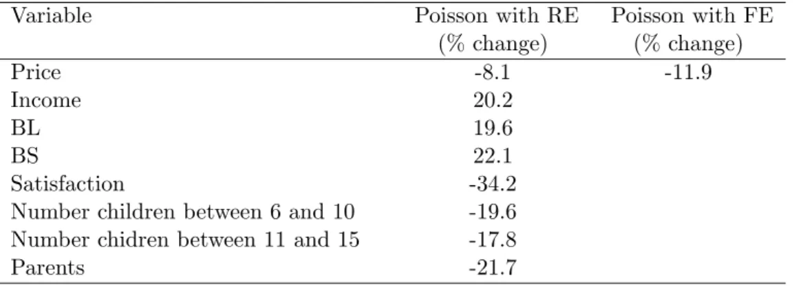
(% change) (% change) Price -8.1 -11.9 Income 20.2 BL 19.6 BS 22.1 Satisfaction -34.2
Number children between 6 and 10 -19.6
Number chidren between 11 and 15 -17.8
Parents -21.7
Table 5: Percentage change in the expected count.
Using equation (5) de…ned in Section 2 to compute the percentage change in the expected count for a -unit change in one of the explanatory variables, we can interpret the impact of the coe¢ cients of the Poisson model with ran-dom e¤ects and …xed e¤ects. We are interested in the percentage change in the expected count for a unit change ( = 1) in the explanatory variable, holding other variables constant. In Table 5 we report the percentage change for the signi…cant coe¢ cients in the Poisson regression model with random e¤ects and …xed e¤ects. The percentage change in the expected count for a unit change in the price of supervised school meals is -8.1% and -11.9%, respectively. This means that an increase in the price of the service by 1 Swiss franc decreases the expected number of services demanded by house-holds by 8.1% or by 11.9%, given the other variables are held constant in the model. Since an increase in the price of the service by 1 Swiss franc roughly
represents a 10% increase in the average level of price (9.92 Swiss francs), this implies that price elasticity of demand is between 0.8 and 1.2, which is not far from the estimated elasticity of 0.4 found by Akin et al. (1983) for the demand for school meals in the US.
As for children’s characteristics and family composition, if the number of additional children between 6 and 10 years and the number of additional children between 11 and 15 years increases by one unit, the demand of super-vised school meals is expected to decrease by 19.6% and 17.8%, respectively. The presence of both parents living in the household reduces the expected number of school meal and childcare services by 21.7%. As for household income, an increase by one unit (that means 2000 Swiss francs) increases the expected quantity of school meal and childcare services demanded by 20.2%, ceteris paribus. Families living in the canton Basel-Country and the canton Basel-City increase the expected number of supervised school meals demanded by 19.6% and 22.1%, respectively, as compared to families living in canton Solothurn. Finally, parents satis…ed with their current care mode are expected to reduce the expected number of school meal and childcare services by 34.2%.
5
Willingness to pay for school meal and
child-care services
The current pricing policy applied by Swiss municipalities for the provision of supervised school meals usually consists of a subsidized price which depends on household income. From the economic point of view, this policy lacks e¢ ciency since cantons and municipalities do not match costs and bene…ts at the margin for the service. Since the service is highly subsidized by local governments, there may be a margin to improve e¢ ciency by taking the willingness to pay for di¤erent categories of consumers into account.
The estimation results of the Poisson model with random and …xed e¤ects can be used to calculate the willingness to pay for supervised school meals. The approach is discussed in details by Haab and McConnell (2002), among
others, who use it to assess the willingness to pay for environmental and natural resources. The willingness to pay can be measured using the integral of the expected demand function estimated by the Poisson regression. The observed dependent variable (Q) is assumed to be a random draw from a
Poisson distribution with mean and the expected demand function is:
E(Q) = . (6)
The value of the willingness to pay equals the area under the expected de-mand curve (6). Using the exponential dede-mand function de…ned by equation
(3) in Section 2, we can write = exp(z p p) + exp( pP ), where P is the
meal price, and z p is a a vector of covariates other than own-price.
De…n-ing P0 as the current meal price, consumer surplus for a meal is obtained
from the integral of the expected demand function. The willingness to pay for (one unit of) the school meal service can then be calculated using the following equation: W T P (meals) = Z 1 P0 ez p p+ pPdP = e z p p+ pP p P !1 P =P0 = p , (7)
when p < 0: Since we want to focus on a daily meal, the willingness to pay
can be derived from (7) as:
W T P (meal) = 1
p
. (8)
Using the estimated parameter of price (^p) from our regressions in
Sec-tion 4, we calculate that the willingness to pay for a daily meal and childcare service is between 7.90 and 11.70 Swiss francs. To our knowledge, this is the …rst attempt to estimate the willingness to pay for supervised school meal services. Consequently, it is not straightforward to compare our valuation with the results of other studies.
For policy discussion, we consider an average cost of approximately 20-25 Swiss francs per unit of service. This value is based on information provided by a Swiss municipality that supplies supervised school meal services. Fur-ther, the average price for a meal and child supervision for households of
medium-income class set by the municipal authority is 12.30 Swiss francs. We observe that our estimated willingness to pay for the service is well be-low the full cost of the service. This implies that the provision of supervised school meal services should be highly subsidized by local governments.
Further, from the pricing strategy point of view, it would be interesting, for instance, to use information on the willingness to pay for di¤erent income categories. To calculate the e¤ect of price for di¤erent income categories, we can slightly modify our Poisson regression with random e¤ects using two approaches. The …rst approach interacts the price variable with a set of dummy variables representing di¤erent income categories, while the second approach introduces a new variable that represents the interaction between price and income.
We estimate these models in order to check whether the willingness to pay for a supervised school meal varies with income. The …rst model considers the interaction between price and three income categories: below 6000 Swiss francs, between 6001 and 8000 Swiss francs, and above 8000 Swiss francs. The second model includes only two income categories: below and above 8000 Swiss francs. Finally, the third model considers the interaction between price and income. Generally, the sign and the magnitude of the coe¢ cients do not vary across the three models, except for price and income interactions. Only the signi…cance of the workload of the respondent di¤ers across the models. In the …rst two models the coe¢ cient of Work is signi…cant, whereas in the third model this is not signi…cant.
The results of the three models are also similar to those of the Poisson regression with random and …xed e¤ects reported in Table 4. The signs of the coe¢ cients are the same. Four covariates improve their level of signi…cance: households living in urban areas, the age of the respondent, the intensity of work (except for the third model where we interact price and income), and the level of education of the respondent. Conversely, the presence of both parents in the family is not signi…cant anymore. Finally, the willingness to pay for school meal and childcare service does not seem to depend on household income since the interaction variables are never signi…cant. Note,
however, that the demand for supervised school meals is signi…cantly and positively a¤ected by household income, which suggests that high-income families are likely to demand more meals per week and, consequently, to spend more for weekly access to school meal services.
We are clearly aware that our estimation of the willingness to pay can be challenged, since the use of stated preferences is exposed to criticism, in particular concerning the techniques to obtain people’s preferences. Stated preference survey techniques usually ask questions about the value for some non-market goods. Therefore, the methods rely on answers to questions about hypothetical situations and the results may be a¤ected by strategic
bias, yea-saying, insensitivity to scope variations and framing.13 The
dif-ference between stated and revealed values is alluded to as a hypothetical bias. We cannot exclude, for instance, that some households underestimated their willingness to pay for school meals to a¤ect future decisions on meals price by cantonal authorities. Also, the hypothetical nature of the survey on payment and provision can result in responses that are signi…cantly greater than actual payments. However, in our case the service is not yet available. Consequently, individuals are not aware of the actual price (revealed value) for the school meal service. Since the meal service was not implemented yet at the time of the survey, we assume that this type of strategic behaviour was negligible. Murphy et al. (2005) point out that despite the richness of studies, there is no consensus about the underlying causes of hypothetical bias or ways to calibrate survey responses for it. In other terms, it is di¢ -cult to understand why people may give a di¤erent willingness to pay on a survey than in an experiment that a¤ects their money (Loomis, 2011). To conclude, although stated preference methods are subject to careful scrutiny, this should not be interpreted as an indication that stated preference esti-mates are less valid than revealed preferences estiesti-mates, as argued by Champ et al. (2003).
13See Bateman et al. (2002) and Champ et al. (2003) for more details.
6
Ordered probit estimations as an
alterna-tive approach
Following Cameron and Trivedi (1986) we consider ordered probit models as an alternative approach to count models used so far in our analysis. Even though the number of school meals appears to be a cardinal measure for school meal services, an ordinal measure approach is also possible. Hence, for instance, two school meals represent a higher level of school meal service than one, but not necessarily 100% more. Consequently, an observed variable of count form may re‡ect a methodological limitation in data collection. This variable is no more than a proxy measured on an ordinal scale. In our case, one could be interested in the use of school meal services rather than the total number of meals during a week. Consequently, if households maximize a utility function, a latent relationship between meals and the explanatory variables can be estimated by ordered models. This approach does not require that events arrive randomly over time according to a well de…ned Poisson process.
As expounded by Maddala (1983), we can treat the observed count
vari-able Qi as a proxy for the variable of theoretical interest, Qi, which by
assumption is assumed to be distributed as N (zi ; 2): Qi is treated as a
categorical variable with J response categories related to the unobserved
variable Qi. The probability of choosing alternative j is de…ned as
Pr(Qi = j) = Pr( j 1 < Qi < j);
1 = 0 < 1 < < J = +1, j 2 f1; 2; :::; Jg , (9)
where js are the threshold parameters. Imposing = 1, the ordinal probit
model leads to the following probability function
Pr (Qi = j) = j zi j 1 zi , (10)
where is the cumulative standard normal density. This equation is at the
basis of the maximum likelihood estimation of parameters j and the vector
.
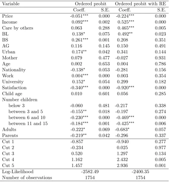
The results obtained using ordered probit regressions with and without random e¤ects are reported in Table 6. It is worth comparing the previ-ous estimates of count data models to those of the ordinal probit model, although the magnitude of the coe¢ cients reported in Table 4 and Table 6 is not directly comparable. We notice that the signs of the estimated
co-Variable Ordered probit Ordered probit with RE
Coe¤. S.E. Coe¤. S.E.
Price -0.051 0.000 -0.224 0.000 Income 0.092 0.002 0.525 0.000 Care by others 0.063 0.288 0.465 0.005 BL 0.138 0.075 0.492 0.023 BS 0.261 0.001 0.208 0.351 AG 0.116 0.145 0.150 0.491 Urban 0.174 0.042 0.341 0.144 Mother 0.079 0.477 -0.027 0.931 Age 0.002 0.653 0.004 0.786 Nationality -0.138 0.053 -0.281 0.156 Work 0.004 0.000 0.003 0.354 University 0.152 0.054 0.299 0.182 Satisfaction -0.340 0.000 -0.920 0.000 Child age 0.010 0.601 0.056 0.285 Number children below 3 -0.060 0.481 -0.217 0.338 between 3 and 5 -0.155 0.018 -0.197 0.274 between 6 and 10 -0.230 0.000 -0.469 0.000 between 11 and 15 -0.184 0.001 -0.425 0.006 Adults -0.222 0.069 -0.683 0.057 Parents -0.219 0.042 -0.296 0.337 Cut 1 -0.857 -0.940 0.277 Cut 2 -0.234 0.025 0.977 Cut 3 0.520 1.297 0.134 Cut 4 1.162 2.432 0.005 Cut 5 1.457 2.936 0.001 Log-Likelihood -2582.49 -2400.35 Number of observations 1754 1754
Note: *, ** and *** denote statistical signi…cance at 10%, 5% and 1% levels.
Table 6: Estimation results of ordered probit regressions.
e¢ cients in the Poisson model with random e¤ects and the ordinal probit
model with random e¤ects are the same. Also, regarding the signi…cance of the coe¢ cients we see little di¤erence. Contrary to Poisson regressions, whether the child is cared by people other than parents is highly signi…-cant in the ordinal probit model with random e¤ects. Living in the signi…-canton Basel-Country (BL) is also more signi…cant (from 10% to 5%) in the ordinal probit model, while living in the canton Basel-City (BS ) and having both parents in the same household are no longer signi…cant. The number of ad-ditional children between 11 and 15 years old increases in signi…cance (from 5% to 1%) in the ordinal probit model. Finally, the dummy indicating that more than two adults older than 15 (Adults) live in the household becomes
signi…cant at 10% level.14 In conclusion, estimations with ordered probit or
logit models do not lead to di¤erent considerations regarding households’ choices of school meal and childcare services, as compared to the estimation approach based on count data models. Therefore, the results in terms of willingness to pay obtained in Section 5 are con…rmed.
7
Conclusions
The provision of extra-familial care services at primary school level in Switzer-land is lacking. However, a growing number of parents, especially mothers, are willing to increase their working time. As discussed in a report by the OECD (2007), an increase in the labour market participation by women is bene…cial not only from the private point of view, but also for the whole economy. To improve the provision of supervised school meal services, the Swiss federal government has extended the program of …nancial incentives to childcare services before, during or after school. To be e¤ective, policy makers need detailed information on the conditions under which parents are willing to use these services.
Using a stated preferences approach, we analysed households’ choices concerning school meal and childcare services for children attending primary
14As a …nal check, we run ordinal logit regressions with and without random e¤ects.
The sign and signi…cance of the coe¢ cients are pretty much the same as in ordered probit models.
school in four Swiss cantons. Our results attest a signi…cant interest for the provision of supervised school meals in primary schools. The number of services demanded during a week depends mainly on the price, the household monthly income, the number of additional children between 6 and 10 years old and between 11 and 15 years old, the presence of both parents in the household, the canton of residence, and the satisfaction with the currently used care mode.
The e¤ect of factors considered in our models may have important impli-cations for the enactment of a school meal and childcare service in the four cantons considered. Our results may help public authorities to understand how di¤erent determinants in‡uence households behavior, which could be taken into account to improve the supply of supervised school meal services. Our empirical study has also two important implications for local policy makers. First, local governments could run de…cits for the provision of meal and childcare services since household willingness to pay is relatively low. Second, although we observe that the number of services demanded increases with household income, we do not …nd evidence that high-income families are willing to pay more than low-income families for school meal and childcare provision during lunchtime. This may suggest that setting a uniform price for supervised school meals which only varies according to household income may not be e¤ective, unless this type of price discrimination is used to redistribute income across income categories for equity reasons.
References
AKIN J.S., GUILLKEY D.K., POPKIN B.M. and WYCKOFF J.H., 1983, ‘The Demand for School Lunches: An Analysis of Individual Partecipation in the School Lunch Program’, The Journal of Human Resources, 18(2), 213-30.
ALBERINI A. and LONGO A., 2006, ‘Combining the Travel Cost and Con-tingent Behavior Methods to Value Cultural Heritage Sites: Evidence from Armenia’, Journal of Cultural Economics, 30(4), 287-304.
ALBERINI A., ZANATTA V. and ROSATO P., 2007, ‘Combining Actual and Contingent Behavior to Estimate the Value of Sports Fishing in the Lagoon of Venice’, Ecological Economics, 61(2-3), 530-41.
BALTAGI B.H., 2008, Econometric Analysis of Panel Data, 4th Edition, West Sussex: John Wiley & Sons Ltd.
BANFI S., FARSI M. and FILIPPINI M., 2009, ‘An Empirical Analysis of Child Care Demand in Switzerland’, Annals of Public and Cooperative Economics, 80(1), 37-66.
BATEMAN I.J., CARSON R.T., DAY B., HANEMANN M., HANLEY N., HETT T., JONES-LEE M., LOOMES G., MOURATO S., ÖZDEMIROGLU E., PEARCE D.W., SUGDEN R. and SWANSON J., 2002, Economic Val-uation with Stated Preference Techniques: A Manual, Cheltenham: Edward Elgar.
BECKER G., 1965, ‘A Theory of the Allocation of Time’, The Economic Journal, 75(299), 493-517.
BEN-AKIVA M. and LERMAN S.R., 1985, Discrete Choice Analysis: The-ory and Application to Travel Demand, Cambridge: The MIT Press.
CAMERON A.C. and TRIVEDI P.K., 1986, ‘Econometric Models Based on Count Data: Comparison and Applications of Some Estimators and Tests’, Journal of Applied Econometrics, 1(1), 29-53.
CAMERON A.C. and TRIVEDI P.K., 1990, ‘Regression Based Tests for Overdispersion in the Poisson Model’, Journal of Econometrics, 46(3), 347-64.
CAMERON A.C. and TRIVEDI P.K., 1998, Regression Analysis of Count Data, New York: Cambridge University Press.
CAMERON A.C. and TRIVEDI P.K., 2005, Microeconometrics: Methods and Applications, New York: Cambridge University Press.
CAMERON A.C. and TRIVEDI P.K., 2010, Microeconometrics Using Stata, Lakeway Drive: Stata Press.
CARPIO C.E., WOHLGENANT M.K. and BOONSAENG T., 2008, ‘The Demand for Agritourism in the United States’, Journal of Agricultural and Resource Economics, 33(2), 254-69.
CHAMP P.A., BOYLE K.J. and BROWN T.C., 2003, A Primer on Nonmar-ket Valuation, Dordrecht: Bateman I.J. ed., Kluwer Academic Publishers. CLARK T.S. and LINZER D.A., 2012, ‘Should I Use Fixed or Random E¤ects?’, Working Paper No. 1315, The Society for Political Methodology. GREENE W.H., 2003, Econometric Analysis, 5th Edition, Upper Saddle River: Prentice Hall International.
HAAB T.C. and McCONNELL K.E., 2002, Valuing Environmental and Nat-ural Resources: the Econometrics of Non-Market Valuation, Cheltenham: Edward Elgar.
HAUSMAN J.A., HALL B.H. and GRILICHES Z., 1984, ‘Econometric Mod-els for Count Data with an Application to the Patents-R & D Relationship’, Econometrica, 52(4), 909-38.
LEE J.-Y., 1987, ‘The Demand for Varied Diet with Econometric Models for Count Data’, American Journal of Agricultural Economics, 69(3), 687-92. LONG J.S., 1997, ‘Regression Models for Categorical and Limited Dependent Variables, Thousand Oaks: Sage.
LONG J.S. and FREESE J., 2003, Regresion Models for Categorical Depen-dent Variables Using Stata, Revised Edition, College Station: Stata Press. LOOMIS J., 2011, ‘What’s to Know About Hypothetical Bias in Stated Preference Valuation Studies?’, Journal of Economic Surveys, 25(2), 363-70. LOUVIERE J.J. and HENSHER D.A., 1983, ‘Using Discrete Choice Models with Experimental Design Data to Forecast Consumer Demand for a Unique Cultural Event’, Journal of Consumer Research, 10(3), 348-61.
LOUVIERE J.J., HENSHER D.A. and SWAIT J.D., 2000, Stated Choice Methods: Analysis and Application, Cambridge: Cambridge University Press. MADDALA G.S., 1983, Limited-dependent and Qualitative Variables in Econometrics, Cambridge: Cambridge University Press.
McCULLOCH C.E., SEARLE S.R. and NEUHAUS J.M., 2008, Generalized, Linear, and Mixed Models, Hoboken: Wiley.
MOON W., FLORKOWSKI W.J., BEUCHAT L.R., RESURRECCION A.V., PARASKOVA P., JORDANOV J. and CHINNAN M.S., 2002, ‘De-mand for Food Variety in an Emerging Market Economy’, Applied Eco-nomics, 34(5), 573-81.
MULLAHY J., 1986, ‘Speci…cation and Testing of Some Modi…ed Count Data Models’, Journal of Econometrics, 33(3), 341-65.
MURPHY J.J., ALLEN P.G., STEVENS T.H. and WEATHERHEAD D., 2005, ‘A Meta-Analysis of Hypothetical Bias in Stated Preference Valuation’, Environmental and Resource Economics, 30(3), 313-25.
OECD, 2004, Babies and Bosses: Reconciling Word and Family Life, Vol. 3: New Zealand, Portugal and Switzerland, Paris: OECD.
OECD, 2007, Babies and Bosses: Reconciling Work and Family Life, A Synthesis of Findings for OECD Countries, Paris: OECD.
PARK J.L. and CAPPS O., 1997, ‘Demand for Prepared Meals by U.S. Households’, American Journal of Agricultural Economics, 79(3), 814-24. PORTNEY P.R. and MULLAHY J., 1986, ‘Urban Air Quality and Acute Respiratory Illness’, Journal of Urban Economics, 20(1), 21-38.
SCHANZENBACH D.W., 2009, ‘Do School Lunches Contribute to Child-hood Obesity?’, The Journal of Human Resources, 44(3), 684-709.
STERN S., BANFI S. and TASSINARI S., 2006, Krippen und Tagesfamilien in der Schweiz. Aktuelle und zukünftige Nachfragepotenziale, Bern: Haupt. THOMAS A., 2000, Économétrie des Variables Qualitatives, Paris: Dunod.