Dynamic light scattering studies of phase transitions in polymers and gels

Dynamic Light Scattering Studies

of Phase Transitions in Polymers and Gels

by

Michal J. P. Orkisz

B.S., Computer Science, Massachusetts Institute of Technology (1988)

B.S., Physics, Massachusetts Institute of Technology (1988)

Submitted to the Department of Physics

in partial fulfillment of the requirements for the degree of

Doctor of Philosophy

at the

MASSACHUSETTS INSTITUTE OF TECHNOLOGY

MAY 1994

© 1994 Massachusetts Institute of Technology

All rights reserved

/ /

AS

2

I

Signature of Author

Department of Physics

May, 1994

Certified By

Accepted By

7

_{Z - ," - \ - I I /}

K

Toyoichi Tanaka

Thesis Supervisor

Gr E

MAR4P"u SEtS INSTI.TUI

' "I My

George F. Koster

Chairman, Departmental Committee

viiY

251994

11

-

DYNAMIC LIGHT SCATTERING STUDIES

OF PHASE TRANSITIONS IN POLYMERS AND GELS

by

Michal J. P. Orkisz

Submitted to the Department of Physics on Apr. 29, 1994 in partial fulfillment of the requirements for the degree of

Doctor of Philosophy in Physics

ABSTRACT

Implementation of a complete system for automated light scattering studies of

gels is described and applied to several gel systems: a neutral homopolymer gel, a

polyelectrolyte, and a polyampholyte exhibiting multiple phase behavior. A logarithmic

software correlator capable of measuring delays from 0.8gs to several hours

simultaneously was designed and used as the core for this system. A method for

estimating correct ensemble averages from time average data collected at different

locations was compiled. A gel description based on collective diffusion and non-ergodic

theories provides basis for interpreting scattering data in terms of dynamic and static

components. The origin of structural inhomogeneities was investigated and found to be

dependent on the pre-gel solution state within the phase diagram at the onset of gelation.

A NIPA (N-isopropylacrylamide) monomer phase diagram was determined to elucidate

the last notion, and found to exhibit a lower critical solution temperature. The critical

point was found to be well below that of a gel. Measurement temperature dependence of

light scattering in a NIPA gel was probed through a discontinuous volume phase

transition. Near-critical fluctuations in both dynamic and static intensities were found

close to the spinodal line. Correlation function shapes confirmed the collective diffusion

origin of dynamic intensity fluctuations. The friction coefficient obtained by light

scattering was found not to vanish near the critical point, contrary to macroscopic liquid flow measurements. A weakly charged NIPA gel was examined and the light scattering results were in agreement with existing SANS data for this gel, confirming the notion of a

microphase separation. A novel dynamic behavior is reported - power law shape of the

correlation function, with a temperature dependent exponent.

A multiple phase

polyampholyte gel (acrylic acid + MAPTAC) was also studied. The pre-gel solution pH was shown to affect gel scattering behavior. The static intensity was found to have two

different concentration dependencies for different pH regions. This demonstrated the

existence of another gel order parameter. Qualitative explanation, based on light

scattering results, was given for some aspects of this gel's complex phase behavior.

Thesis Supervisor:

Dr. Toyoichi Tanaka

'AD MAIOREM DEI GL ORIAM"

I WOULD ALSO LIKE TO DEDICA TE THIS THESIS

TO MYPARENTS:

JANUSZAND MARIA ORKISZ

AND TO MY 'ADOPTED MOTHER"

ACKNOWLEDGMENTS

First I would like to thank my supervisor, Dr. Tanaka. There are many reasons for my gratitude: his supervision, his encouragement, his patience, and last, but not least, his faith in me that in many cases exceeded my faith in myself.

I am grateful to my many colleagues and co-workers I encountered in Prof.

Tanaka's group during my several years' sojourn here. I list them in an alphabetical

order: Dr. Masahiko Annaka, Anthony English, Dr. Sid Gorti, Prof. Alexander Grosberg, Dr. Terrance Hwa, Dr. Frank Ilmain, Prof. Etsuo Kokofuta, Dr. Yong Li, Dr. Toyoaki Matsuura, Vijay Pande, Bill Robertson, Prof. Mitsuhiro Shibayama, Prof. Ron Siegel, Dr. Masayuki Tokita, Kevin Wasserman, Prof. Shigeo Yoshino, Dr. Xiaohong Yu, and Dr. Yong-Quing Zhang.

I want to thank my parents and the rest of my family. They know best what I need to be grateful for, and anyone else can use his or her imagination.

Last but not least, I want to extend my thanks to all of my C&L friends at MIT, in Boston, in the USA, and all over the world. Foremost among them to my "adopted mother". Dr. Ana Lydia Sawaya, without whose encouragement to take my life seriously I would probably have not finished this thesis.

TABLE OF CONTENTS

IN TRO DU CTIO N ... 15

0. 1 Gels ... 15

0.2 Gel Phase Transitions ... 16

0.2.1 Fundamental Forces ... 18

0.2.1. 1 van der Waals Interaction ... 18

0.2.1.2 Hydrophobic Interaction ... 18

0.2.1.3 Hydrogen Bonding ... 18

0.2.1.4 Electrostatic Interactions ... 19

0.2.2 Flory-Huggins Theory of Gel Phase Transitions ... 19

0.3 Light: Scattering ... 21

0.3.1 Overview ... 21

0.3.2 Scattering Geometry ... ... 21

0.3,3 The Correlation Function ... 22

0.4 The Apparatus ... 23

0C.4. 1 Overview ... 23

0.4.2 Sample Holders ... ... 25

0.4.3 Sample Translation ... ... 26

0.5 About this Thesis ... 27

0.5.1 Motivation ... 27

0.5.2 Organization ... 28

0.5.3 Specific Contributions

...

29

References ...

...

31

1. DESIGN AND IMPLEMENTATION OF A SOFTWARE CORRELATOR ... 33

1.1 Introduction ... 33

1.2.1 Definition ... 34 1.2.2 Discrete Approximation ... 35 1.2.3 Graphical Representation ... 37 1.2.4 Sources of Errors ... 37 1.2.4.1 Decimation ... 38 1.2.4.2 Discretization ... 39

1.2.4.3 Finite Collection Time ... 41

1.3 Software design ... 41 1.3.1 Why Logarithmic? ... 41 1.3.2 Principle of Operation ... 42 1.3.3 Main Loop ... 44 1.3.4 Initialization ... 45 1.4 Data compression ... 46 1.5 Hardware design ... 46

1.5.2 BI-2030AT as a Front End ... ...48

1.6 Analysis Software ... 49

1.6.1 Ensemble Averaging ... 49

1.6.2 Curve Plotting and Fitting ... 50

Summary

...

51

References

...

51

2. LIGHT SCATTERING FROM NON-ERGODIC SYSTEMS ... ... 53

2.1 Overview of (Non)ergodicity ...

53

2.1.1 Ensemble vs. Time Average ... 54

2.1.2 Ergodic vs. Nonergodic Systems ... 56

2.1.3 Light Scattering ... 56

2.2.1 Different Approaches ... 59

2.2.2 Correcting the Effects of Finite Averaging ... 60

2.2.2.1 Underlying Assumptions .

...

61

2.2.2.2 Estimating the Deviation ... 62

2.2.2.3 Correcting the Deviation ... 63

2.3 Theory of Light Scattering in Gels ... 67

2.3. 1 Origin of the Static Component ... 67

2.3.2 Collective Diffusion and the Origin of the Dynamic

Component ...

69

2.3.3 Summary ... 71

2.4 Some Experimental Results ... 71

2.4.1 Correlation Function Statistics ... 71

2.4.2 Speckle Pattern ... 73

2.4.3 Reproducibility ...

74

2.4.4 Randomness ... 75

2.4.5 Intensity Histogram ... 76

2.4.6 Local Oscillator Effects (Heterodyning) ... 77

2.4.7 Extracting Decay Time from Ensemble Average ... 78

Conclusion ...

80

References ...

81

3. FROZEN GEL INHOMOGENEITIES - TEMPERATURE OF GELATION DEPENDENCE ... 83

3.1 Introduction ... 84

3.2 Experiments ...85

3.2.1 Sample Preparation ... 85

3.3 Results ... 86

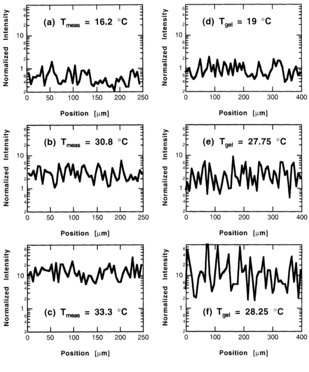
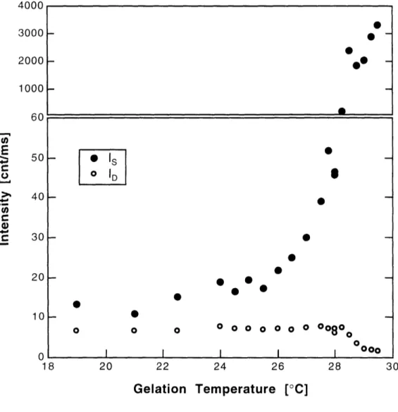
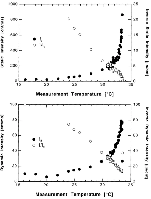
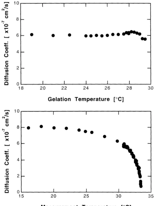
3.3.1 General Observations ... 86

3.3.2 Dependence on Gelation Temperature ... 89

3.3.3 Dependence on Measurement Temperature ... 89

3.4 Discussion ... 94

C onclusions ... 97

Further Research ...

98

References ...

99

4. PHASE DIAGRAM OF NIPA MONOMER ... ... 101

4.1 Introduction ... 101

4.2 Experiments ... 102

4.2.1 Liquid-Liquid Phase Boundary ... 104

4.2.2 Solid-Liquid Phase Boundary ... 104

4.3 Results ... ... 104

4.4 Discussion ... 106

Conclusion ...

.

...

110

Further Research ... 110

References ... 111

5. LIGHT SCATTERING FROM A NIPA GEL NEAR A TEMPERATURE INDUCED PH A SE TRANSITION ... 113

5.1 Introduction ...

.

...

113

5.2 Experiments ...

.

...

115

5.2.1 Sample Preparation ... ... 115

5.2.2 Temperature ... ... 115

5.2.3 Approach to the Transition ... 115

5.3 Results ... 117

5.3.1 The Transition ...

117

5.3.2 Correlation Functions ...

...

1...

118

5.3.3 Light Scattering Results ... 120

5.4 Discussion ... 120

5.4.1 Shape of the Correlation Function ... 120

5.4.2 Near-Critical Behavior ... 124

5.4.3 Network-Solvent Friction ... ... 128

Conclusions ...

...

131

Further Research ... 131

References ... 132

6. LIGHT SCATTERING FROM A POLYELECTROLYTE GEL ... 133

6.1 Introduction ... 133 6.2 Experiments ... 137 6.2.1 Sample Preparation ... 137 6.2.2 Temperature ... 137 (.2. 3 Light Scattering ... 137 6.3 Results ... ... 139 6.3.1 Scattering Parameters ... 139 6.3.2 Intensities ... 142 6.4 Discussion ... 142

Conclusion ...

146

Further Research ... ... 147 References ... ... 148

7. ANALYSIS OF A MULTIPLE-PHASE POLYAMPHOLYTE GEL ... 149

7.1.1 Organization of this Chapter ... 152

7.1.2 Sample Preparation ... 152

7.1.3 Temperature ... 154

7.1.4 Light Scattering ... 154

7.2 "Unwashed" gels - Dependence on Preparation Conditions and

Composition ...

155

7.2.1 Experiments ... 155

7.2.2 Results ... 155

7.2.3 Discussion ... 158

7.3 "Constrained" gels - Diameter Dependence ... 159

7.3.1 Experiments ... 159

7.3.2 Results ... 160

7.3.3 Discussion ... 163

7.4 Comparison of Unwashed, Constrained, and Free gels ... 165

7.4.1 Experiments ... 165

7.4.2 Results ... 167

7.4.3 Discussion ... 168

7.5 "Free" Gels - pH Dependence ... 169

7.5.1 Experim ents ... 169

7.5.2 Results ... 169

7.5.3 D iscussion ... 171

Conclusions ...

178

Further Research ...

...

179

References ... ... 181 FURTHER RESEARCH ... 183 CO N CLU SIO N ... 187

INTRODUCTION

This thesis deals with light scattering studies of phase transitions in polymer gels. I shall start by briefly describing these terms in reverse order: first gels, then gel phase transitions, then the light scattering technique. Subsequently, the apparatus used in most

of the experiments reported here will be described. Finally, some information about the

organization, and an evaluation of this thesis will be given.

0.1 GELS

A polymer gel is a three-dimensional polymer network in contact with a solvent. The polymers can be of any nature: biopolymers such as proteins or DNA or synthetic

polymers. The gels investigated in this thesis are exclusively synthetic. Component

chains can be linked by physical means (such as entanglements, hydrogen bonding), or

covalent crosslinks (i.e., chemical bonds). This thesis deals only with chemically

crosslinked gels. An interesting aspect of such gels is that the whole gel is a single

molecule of macroscopic size. They are an ideal medium for studying molecular

interactions, as the effects of microscopic inter-polymer forces manifest themselves on a

macroscopic level.

Gels are abundant in nature. Many of the living tissues, such as the cornea,

vitreous humor, the connective tissues, basement membranes, liners of stomach and lung

surfaces, etc., exist in a gel form. Gels are widely used in scientific, industrial, and

everyday life contexts. Their applications range from a medium for macromolecule

separation by electrophoresis or liquid chromatography in biology, "breathable" materials

for soft contact lenses, super absorbent fillers of disposable diapers, slow release carriers

of drugs in medicine, and many others. New research in "intelligent gels" promises

future applications in molecular recognition (artificial enzymes), mechanical actuators

(artificial muscles), controlled drug release (drug release in response to chemical changes in the organism), information storage (holographic memories), etc.

Fig. 1 Schematic drawing of a gel. Black lines represent the polymer chains, white circles the crosslinks, and gray background the solvent.

To realize these potential applications and other future developments it is

important to understand the microscopic structure of gels. One of the goals of this thesis is to make a contribution towards this understanding.

0.2 GEL PHASE TRANSITIONS

The phase transitions discussed in this thesis are volume phase transitions. Figure 2 illustrates such a transition. The topology of the network remains the same (the number and the placement of crosslinks does not change), but the conformation and density of the chains changes. Solvent is expelled from the network in the process. This is a phase

transition in the usual sense of the word (see, e.g., (1)). An infinitesimal change in

external conditions can trigger a macroscopic change in the gel. Volume changes of up to

1000 times have been observed. The change is fully reversible, i.e., when the initial

conditions are restored the gel returns to its former state.

Fig. 2 Volume phase transition of a gel. The network collapses - the

chains become more densely packed, and the solvent is expelled.

Volume phase transitions can be contrasted with another class of transitions

closely related to the gel state: sol-gel transitions. In the latter case, a solution (of finite

viscosity) becomes, through the process of crosslinking, a gel (of infinite viscosity).

These transitions, although interesting in their own right, are not dealt with in this thesis.

The possibility of a gel volume phase transition was first predicted theoretically by Dusek and Patterson in 1968 (2). A physical manifestation of such a transition was not observed till almost 10 years later. In 1977 Tanaka for the first time observed a

volume transition of a slightly ionized acrylamide gel in an acetone-water mixture (3).

Since then many factors that induce phase transitions have been discovered: temperature

(4), solvent composition (5,6), solvent pH (7), electric field (8), external pressure (9),

ultraviolet (10) and visible light (11), and specific molecules (12).

The interested reader is referred to (13-14) and references therein for a much more exhaustive discussion of polymer gels and gel phase transitions.

I%-0.2.1 Fundamental Forces

Gel phase transitions result from a competition between attractive and repulsive

forces attempting to collapse and swell the gel. Listed below are the four fundamental

forces responsible for molecular interactions (N.B. all are a manifestation of the

electromagnetic force), which in gels compete with entropic forces manifested in

gel-solvent mixing entropy and rubber elasticity.

0.2.1.1 van der Waals Interaction

The van der Waals interaction is present in every system. It is a multipole

-induced multipole attraction (accompanied by short range excluded volume repulsion).

Therefore its strength in water is usually much smaller than other interactions, and it can be ignored. However, a change in solvent composition can make it more pronounced.

The first volume transition ever observed (3) was in fact induced by van der Waals

attraction.

0.2.1.2 Hydrophobic Interaction

Hydrophobic interaction between polymer chains and water is an entropic force.

Water molecules in the vicinity of a hydrocarbon group become more ordered (ice

structure) than in pure water. Thus the entropy is lowered. In order to maximize the entropy the chains are forced to aggregate. The lowered chain entropy is compensated by

the gain of entropy by water. This effect is stronger at higher temperatures, so

hydrophobic gels tend to collapse when heated. The transition described in (4) is driven by a hydrophobic interaction.

0.2.1.3 Hydrogen Bonding

Hydrogen bonding is an attractive interaction due to formation of hydrogen bonds

between polymer chains. The energy of a hydrogen bond is significantly smaller than

that of a covalent bond, so the bonds can form and break as the temperature is decreased and increased. Reference (16) reports a phase transition driven by hydrogen bonding.

0.2.1.4 Electrostatic Interactions

Several effects are due to electrostatic forces between charged polymer chains

themselves and between the chains and mobile counterions in the solution. If the network carries a net charge the osmotic pressure of counterions attempts to swell the gel. The is

Coulomb repulsion between like network charges is usually screened by water. In the

case of a polyampholyte gel, where both positive and negative charges are attached to the network, long range attractive forces are present (see Reference (17) for a more extensive

treatment).

0.2.2 Flory-Huggins Theory of Gel Phase Transitions

The classical theory of gel phase transitions is based on the Flory-Huggins form

of fiee energy (2). In this summary it is assumed that the swelling force is due to the counterion pressure (13). The free energy can be decomposed into three parts:

F = Fmixing + Frubber elasticity + Fcounterion

These terms can be expressed explicitly as:

vkT

(each term corresponding to the one above) where N is the total number of persistent units, v the total number of chains (bounded by crosslinks), X is the reduced chain-solvent interaction energy (Flory parameter), ¢ is the network volume fraction (¢o - the reference state - is the volume fraction when the chains are Gaussian - usually the concentration at which the gel was polymerized), and f is the charge per chain. When a gel is freely swollen, its osmotic pressure 7r is zero. Thus the swelling behavior can be analyzed by considering the isobars: =

p

2(OF / a3) = 0.

Performing the calculations and expanding the logarithms to order

p

3

_{, the}

following simplified equation is obtained: t = S (p- 5 /3 -p- /2)-p/3 with the reduced parameters defined as

(1- 2x) (2f + 1)3 / 2

t

--P- /--' (2f + 1)3 /2

S

v- '(2f

+1) 4

Analyzing this equation we observe that for S larger than Sc=234.1 the isobar has a Maxwell loop, and the transition becomes discontinuous. Figure 3 (reprinted from (13)) shows the swelling curves (parametrized by f) obtained from this equation.

12

2

a

-. W -0_ID Er 10-2 10-1 100 101

Degree of swelling (V/Vo)

IOz

Fig. 3 Theoretical swelling curves for various degrees of ionization f

(number of ions per chain), based on the Flory-Huggins formula. (Reprinted from (13)).

This model does not give correct quantitative results, but at least it can

qualitatively predict existence of discontinuous volume phase transitions. The reader is

referred to (13-15) for more details.

0.3 LIGHT SCATTERING

0.3.1 Overview

Many books have been devoted to the theory and practice of laser light scattering (see, e.g., (18-20)), so I will confine myself to essentials.

Light passing through a medium is scattered by density fluctuations (or, more

precisely, by refractive index fluctuations). Scattered light is then detected and analyzed. This follows the general scheme of most techniques available to physicists today - be it condensed matter, atomic, or high energy. The sample is hit or probed with something

and the response is observed. In our case the sample is a gel, and the probe is light. Here

the incident light does not perturb the sample - it only probes the ever-present thermal

fluctuations of the system.

It is interesting to note an exact analogy between a light scattering experiment and

the principle of FM radio.

The carrier wave of the radio corresponds to the

monochromatic incident laser light. This carrier is frequency modulated by another

process of much lower frequency - either by an audio signal, or by the thermal

fluctuations inside a sample. The modulated wave is transmitted through space to a

detector - ideally a so-called perfect square-law detector. This is implemented in a radio

receiver using an antenna and electronics. In the case of light scattering this role is

played by the surface of the photomultiplier tube (PMT), which is sensitive to intensity of the incident light -- exactly the square of the incident electric field. The signal is then

demodulated. In a radio receiver the voice or music is recovered, while in the case of

light scattering it is the fluctuating signal of the sample. Actually, we are not interested in the signal itself, but rather in its signature obtained with the aid of an autocorrelator.

0.3.2 Scattering Geometry

Figure 4 illustrates the scattering geometry. Laser light passing through the

sample is scattered (in all directions). Light scattered at an angle 0 with respect to the beam direction is picked up by the detector.

Incident laser light of wavelength X (in vacuum) is described by wave vector ki, where Ikl = 2n/k, where n is the refractive index of the medium. The scattered light's wave vector has the same magnitude Ikl, but different direction kf. Their difference gives the scattering vector q = kf - ki, whose magnitude is, from the law of cosines,

q = sin ,

X

-Throughout this thesis we use a fixed 90

°

angle and a He-Ne laser, with a vacuum

wavelength k=633nm. The resulting scattering vector magnitude is q=70 nm-

1

.

I spr

Sample

kf\

Detector

Fig. 4 Scattering geometry. Incident laser light is scattered by the sample and detected at an angle 0. The construction of the

scattering vector q is also shown.

0.3.3 The Correlation Function

The way of extracting information from the scattered light is by measuring the

autocorrelation function of the scattered light intensity. The time-averaged normalized

intensity autocorrelation function C(t) is defined as:

C(t)

(I(t') I(t' +t))

(I(t'))

2

where I(t) is the instantaneous intensity measured at time t. If I(t) and I(t+At) can be considered independent for Ate0, as in the case of Poisson statistics (normal light source), or for At much greater than the internal relaxation time (for any fluctuating system), then the average of the product I(t)-I(t+At) equals the product of the averages, so C(t)= 1. Thus one would expect the limit of C(t) for large t to be 1. On the other hand, at t=0 we have

C(0)=(I2)/(I)2, so C(O) is related to the second moment of intensity distribution. For an electric field with Gaussian distribution (as one would normally expect), we have C(O)=2. The information conveyed by the correlation function is the same as in the power spectrum of the signal. In fact they are related to each other by a Fourier transform.

0.4 THE APPARATUS

This section describes the light scattering setup used for all of the light scattering experiments presented in this thesis. An overview is given first, and specific details are given later. In particular, the sample holders, the temperature control, and the sample

translation are discussed. The core of the setup - the software correlator - is not

described here since Chapter 1 is devoted to it.

0.4.1 Overview

The setup used throughout this thesis differs from a conventional light scattering apparata (in design, not in principle). It is a Microscopic Laser Light Scattering (MLLS) setup (see Figure 5) where a microscope is used to observe the sample and to detect the

scattered light. This particular setup was originally devised for performing light

scattering experiments in microscopic biological samples. This setup was modified and

adapted for scattering from gels since it offered several advantages over a conventional (optical table size) setup. First, it allows for precision measurements to be performed on small size samples. This is very important since the speed of a gel transition decreases

quadratically with increasing size. Thus the speed gain from using samples of order

0.5mm (MLLS) as opposed to 5mm (conventional setup) is 100-fold. This translates to

minutes versus days. The apparatus was also particularly amenable to installing a

stepping motor for moving the sample under observation. This is important in gel light scattering measurements since gels are non-ergodic and one cannot equate the ensemble average with a time average of a measured signal. The ensemble average can be obtained by collecting data at different points.

There are two main disadvantages of our MLLS setup. The scattering angle is fixed. (A 90° angle was used since it was the most natural choice given the sample

geometry - see Figure 6.) This precluded the possibility of running angular dependence

experiments, which could have shed more light on the structure of the systems under

investigation. The other deficiency is that ideally the detector should be point-size. In

practice, however, the finite size of the aperture of the objective lens extended the

effective detector size, so that the scattering parameter

(more about its meaning in

chapter 2) was 0.8 as opposed to the ideal value of 1.0 (actually, our conventional setup had an even lower value of

3).

Microscol:

GRIN I

PMT)

Beam

Optic fiber

Sample

(from laser)

(in couvette)

Fig. 5 Schematic diagram of the Microscopic Laser Light Scattering

(MLLS) setup. The light from a laser is brought through a single

mode optic fiber and focused with a GRIN lens. The scattered light is collected through microscope's optics and transmitted, through another optic fiber into the detector (a PMT)

Figure 5 illustrates the light scattering setup. The source of light was a Spectra Physics He-Ne laser (model 127) with an output power of -50mW. The optics for delivering laser light to the sample were custom made by OZ Optics Ltd. The light was fed into a single-mode fiber using an OZ Optics coupler, and on exit focused by a GRIN (Graded Refraction INdex) lens 4mm away from the lens surface. This in practice gave a

focused waist of under 10gm in diameter. Some light was lost during the transmission,

so the output power from the GRIN lens was reduced to about 20mW.

Figure 6 shows the scattering geometry. Scattered light (going up in the figure) is picked up through a Nikon OPTIPHOT microscope. It was equipped with a Leitz L32

long working distance objective lens (with adjustable aperture) and Gamma Scientific

10x eyepieces with built-in optical fiber in the focal plane (model 700-10-36A with 50gm

fiber and 700-10-37A with 150gm fiber). The larger fiber was normally used. If the

scattering intensity was too high, the 50gm fiber was employed. The light from the

eyepieces traveled through a shielded fiber bundle to a photomultiplier tube operated in a photon counting mode. The pulses from the PMT were converted to TTL levels and fed into a correlator, which is described in detail in Chapter 1.

Scattered light

Temperature

bath

Micropipette

Mooie

Icmn

Motorized

A/

motion

Incoming

motion

beam

beam

Fig. 6 Actual scattering and sample geometry

0.4.2 Sample Holders

Several sample holders were used depending on the conditions of the experiment.

The simplest measurements were performed at room temperature measurements with no

change in the gel environment. In this case the gel was kept in a round micropipette

inserted into a square cuvette (10mm x 10mm) of optical quality glass (available from

many glass manufacturers, e.g., Helma). The micropipette was held in place by rubber

spacers. The cuvette was filled with water to minimize the lens effect of the micropipette and plugged with a square rubber stopper. This arrangement is represented in Figure 6.

In some cases the environment in which the gel was placed had to be changed

during the experiment. In a series of measurements, for example, the solution pH was

monitored and varied. In this case the gels were allowed to swell freely as the solution flowed around them. They were held in place at one end by the micropipette in which they were made. Full description is provided in Chapter 7 where this holder is used.

Finally in some experiments the temperature had to be changed. The simplest solution would be to run water from a heat/refrigeration bath (such as Neslab or Lauda) through a cuvette holding the micropipette, as described above. However, the flow from the heat bath introduces vibrations that were picked up through light scattering and affect the correlation function. Therefore this solution is impractical. So a metal (copper in one version, aluminum in another) sample holder with glass windows was constructed, inside which the micropipette was immersed in water, as before. The holder sits on top of two

thermoelectric devices connected to one of the temperature control units available in the

lab (and constructed by a previous generation of graduate students). The controller uses a

thermistor in a Wheatstone bridge configuration. The imbalance between the two

branches of the bridge is presented to the input of an integrator (with adjustable gain and

time constant), whose output, after amplification, drives the thermoelectric devices. This

configuration was altered in such a way that the reference part of the bridge was replaced

with the output of a DAC (Digital to Analog Converter) form Keithley System 570

controlled by the computer. Another thermistor was read by Keithley's ADC. so the temperature could be both controlled and monitored by the computer.

0.4.3 Sample Translation

All sample holders are mounted on an X-Y translation stage. The micrometric screw controlling the X stage was attached to a stepping motor which moves the stage back and forth. Stepping motors rotate their shafts in exact increments when the voltage applied to their coils is circled through 4 phases. The particular motor used had 200 steps

per revolution, which, combined with 0.5mm per revolution pitch of the micrometer

screw, provides a resolution of 2.5rm per step. A stepping motor controller was

constructed. It translates the signals from a parallel port of an IBM PC compatible

computer into 4 phases. They are amplified through power transistors to drive two

independent stepper motors. (The other motor was sometimes used to re-center the beam

during long measurements.) Thus the position could be controlled from the same

computer that collected the correlation function and controlled the temperature.

The only other complication was that each motor step would jerk the stage, and

shake the sample. Since the sample had to be perfectly still for light scattering

measurements, this had to be avoided (especially in cases when the sample was floating

almost freely). The solution adopted was to oscillate the motor rapidly (-7kHz) between

two consecutive steps, and to vary smoothly the oscillation duty cycle. As the

oscillations are much faster than motor's response time, this results in a smooth transition between the two positions.

0.5 ABOUT THIS THESIS

The following three sections describe this thesis. First the motivation behind this research is stated, then the conceptual organization is described. Finally a critical look is taken where author's contributions are stated and the relevance of the findings discussed.

0.5.1 Motivation

A property of gels which sets them apart from most other substances is that they combine both liquid and solid nature. A liquid, even as complex as a polymer solution, does not exhibit any permanent structure. The solvent particles are free to move around,

even if it happens very slowly. A solid, on the other hand, can have a permanent

structure. Positions of individual particles are fixed in space and time except for the

thermal oscillations about the equilibrium positions. A gel, on the other hand, consists of polymer chains that are mostly free to move around (as in a liquid), but there are some limitations because the chain ends are linked to other chains. Beyond the conformational

motion of the chain whose end points are fixed, the movement involves a collective

displacement of the whole network. A network can have many imperfections - dangling

ends, loops, regions of higher crosslinking density, etc., - all of which influence the

structure of a gel. These are structural inhomogeneities. In addition, other

inhomo-geneities can be formed dynamically by the monomer interactions.

These inhomogeneities play an important role in the optical, mechanical,

theological, etc., properties of gels. They also influence the gel phase behavior. What is

even more important, the inhomogeneities are related to the memory of structure.

Random polymers are free to change their conformation and relative positions. They do not exhibit any memory. Certain biopolymers, especially the proteins that play a crucial role in life processes, can "remember" their structure. They exist in one, or at most a few conformations. When pushed out of this state, they can find it again (thermodynamic

renaturation). The structure of some proteins, such as enzymes and antibodies, enables

them to lock onto specific targets (molecular recognition). Frozen inhomogeneities

provide gels with at least a trivial form of shape memory - densely crosslinked regions

remain dense, while dilute regions stay dilute. Can this memory be more specific? Can a gel, or at least its portion, find a particular "frozen" state? Would this state be unique? Can it be reached again after the gel was swollen? Would it be possible to design such a

state? Can it be made to recognize specific targets? Such structure, if existent, would

also be a form of a structural inhomogeneity.

To answer these questions it is important to understand the physical principles of

their formation and to characterize the inhomogeneities. This thesis attempts to do this.

It investigates a mechanism by which thermal fluctuations become frozen as

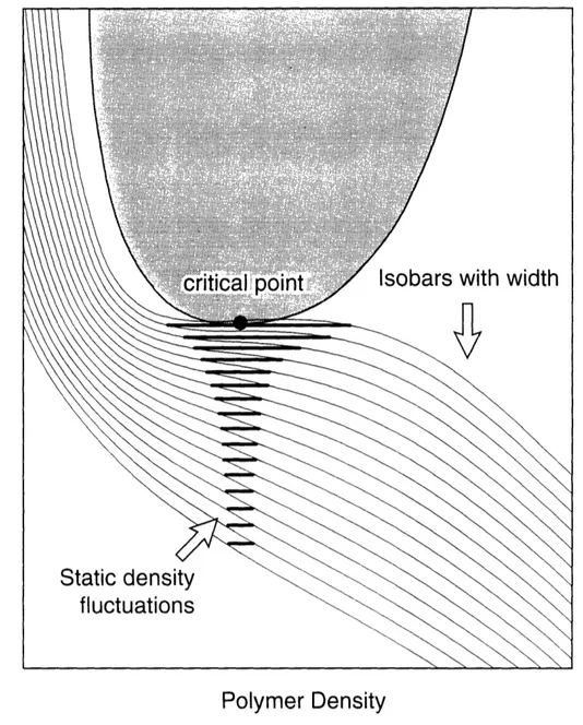
inhomogeneities. It traces the divergence of these inhomogeneities at the spinodal line.

Finally, it investigates the dynamic and static nature of inhomogeneities caused by

interactions among monomers.

0.5.2 Organization

The thesis begins by describing the logarithmic correlator, used extensively in the

experiments reported here, as a part of the light scattering setup described in this

introduction. The second chapter presents the theory and practice of analyzing light

scattering data. The following chapters describe the actual experiments. The progression

is from relatively simple systems (neutral gels), through a more complicated

polyelectrolyte gel (network charged with ions of one polarity), to a polyampholyte

(network with both anionic and cationic components). More precisely, the third chapter

deals with the formation of inhomogeneities during the gelation process (probed by light

scattering) of an N-isopropylacrylamide (NIPA) gel. The fourth chapter determines the

phase diagram of NIPA monomer, which is necessary to elucidate the results of the third

chapter.

The fifth chapter examines light scattering from a NIPA gel near a

discontinuous phase transition. The sixth chapter examines the behavior of NIPA with

ionizable units of acrylic acid added to make it a weak polyelectrolyte. Finally, the

seventh chapter reports various aspects of scattering from a polyampholyte gel

-copolymer of acrylic acid and MAPTAC.

0.5.3 Specific Contributions

All the experiments presented in this thesis were performed by the author (with the exception of several figures reprinted from elsewhere and marked as such). The core of the microscopic light scattering apparatus was neither designed nor built by the author.

However, significant modifications and additions were done by the author to convert it

from a system prepared to measure biological samples to one suitable for the study of

gels. In particular, the optics were redesigned, the sample holders, temperature

controllers and the motorized stage designed, constructed, and tested. This setup offers unique advantages in studying microscopic size gels.

The logarithmic software correlator described in Chapter 1 is the fruit of several

hardware designs conceived by the author (but never implemented) in an attempt to

create a simple and inexpensive correlator suitable for use in clinical eye testing

equipment. The idea of a logarithmic correlator implemented partially in software is not new. In fact there exist some commercial designs. However this correlator was designed

and implemented entirely by the author. Its main advantages are very low cost of

necessary hardware, and its integration into a larger system for collecting and analyzing

gel light scattering data (also designed and implemented entirely by the author).

The theoretical considerations presented in Chapter 2 are neither new, nor due to

the author. However, the resulting procedures for extracting information from the

scattering data and correcting for errors due to averaging over a finite set of data are

derived by the author. So is the attempt to combine the collective diffusion with the non-ergodic approaches, which is later successfully (at least for simple systems) applied to the actual data.

The main ideas in Chapter 3 (about the origin of gel inhomogeneities) are not due to the author. All the experimental results are his, though. Among them of greatest value are the precise temperature of gelation measurements and their decomposition into static and dynamic components.

All of Chapter 4 is the author's work, including the data, its analysis, and the simple model explaining the results. This work furnishes important evidence supporting the ideas presented in Chapter 3.

Some of the light scattering experiments presented in Chapter 5 were performed

in the past by other researchers. Therefore part of the experimental data repeats previous

results. However, author's results are more precise and a more thorough analysis of the

data (using the methods devised in Chapter 2) reveals some interesting new aspects. In

addition the author was able to perform light scattering from a collapsed NIPA gel, which is a new result. This, combined with the data from swollen gel, gives a clearer look at the

discontinuous transition.

The experiments described in Chapter 6 originated in conjunction with Small

Angle Neutron Scattering experiments performed by Dr. M. Shibayama on the same gel.

The light scattering study was performed entirely by the author. The observations

presented in that chapter are new. Especially interesting is the power law shape of the

correlation function and its temperature dependence at higher temperatures. The

observation of power law behavior in this context is new. Unfortunately, the author

failed to find any quantitative arguments that would model this behavior, so only an

attempt is made to explain it qualitatively.

The experiments described in Chapter 7 originated in collaboration with Dr. M. Annaka in the process of his study of the multiple-phase gels. However, the results in

Chapter 7 do not deal explicitly with the multiple-phase behavior (because of the

difficulty of performing light scattering at the low concentrations of the multiple phases). Instead they reveal some interesting aspects of dependence on preparation conditions and

explicitly demonstrate the existence of another order parameter (besides density) in a

charged gel, which is an important finding. (N.B. the experiments presented in this

chapter, more than any other ones, testify to the usefulness of the microscopic light

scattering setup in studying gels, since they would be practically impossible to obtain

with macroscopic gels.)

REFERENCES

[1] Huang, K.: Statistical Mechanics, Wiley & Sons, New York, p 34ff (1963). [2] Dusek, K. and Patterson, D.: J. Polym. Sci. Part A-2, 6, 1209 (1968).

[3] Tanaka, T.: Phys. Rev. Lett., 40, 820 (1978).

[4] Hirokawa, Y. and Tanaka, T.: J. Chem. Phys., 81, 6379 (1984).

[5]

Tanaka, T., Fillmore, D., Sun, S.-T., Nishio, I., Swislow, G. and Shah, A.: Phvs.

Rev. Lett., 45, 1636 (1980).

[6] Ilavsky, M.: Macromolecules, 15, 782 (1982). [7] Tanaka, T.: Sci. Am., 244, 124 (1981).

[8] Tanaka, T., Nishio, I., Sun, S.-T. and Ueno-Nishio, S.: Science, 218, 467 (1982). [9] Suzuki, A.: 4th Gel Symp., Tokyo (1990).

[10] Mamada, A., Tanaka, T., Kungwatchakun, D. and Irie, M.: Macromolecules, 23, 1517 (1990).

[11] Suzuki, A. and Tanaka, T.: Nature, 346, 345 (1990).

[12] Kokofuta, E., Zhang, Y.-Q. and Tanaka, T.: Nature, 351, 302 (1991). [13] Li, Y. and Tanaka, T.: Annu. Rev. Mater. Sci., 22, 243-277 (1992).

[14] Tanaka, T., Annaka, M., Ilmain, F., Ishii, K., Kokofuta, E., Suzuki, A. and Tokita, M.: NATO ASI Series, Vol. H64, pp. 683-703 (1992).

[15] Shibayama, M. and Tanaka, T.: Adv. in Polymer Sci., 109, 1-62 (1992).

[16] Ilmain, F., Tanaka, T. and Kokofuta, E.: Nature, 349, 400 (1991). [17] Yu, X.H., Ph.D. Thesis, M.I.T (1993)

[18] Chu, B.: Laser Light Scattering, Academic Press, London (1991 ).

[19] Berne, B.J. and Pecora, R.: Dynamic Light Scattering, Wiley & Sons, New York, (1976).

1[20] Tanaka, T., "Light Scattering from Polymer Gels" in Dynamic Light Scattering, ed. R. Pecora, Plenum Publishing Co., New York (1985)

CHAPTER 1

DESIGN AND IMPLEMENTATION OF

A SOFTWARE CORRELATOR

This chapter provides details of design and implementation of a logarithmic

correlator and its supporting software and hardware. This instrument was used throughout

the rest of this thesis for collecting light scattering data.

1.1 INTRODUCTION

The dynamic light scattering technique is a powerful method of examining the

structure of solutions and gels. It can provide information about phenomena taking place at very different time scales. For example, a typical gel might exhibit a decay time of

10-100gs. On the other hand, the speckle pattern in such a gel is much more permanent, in

some cases not changing on the time scale of days and larger. Several observed

phenomena exhibited a correlation function displaying a power-law decay, which does

not have a characteristic time scale at all. The need to examine such a wide range of time scales at the same time dictated the necessity to go beyond the equally spaced 136

channels of a typical linear correlator. It is true that the Brookhaven Instruments'

BI-2030AT available to me has a so-called multiple-tau option in which four banks of 32 channels can be set to separate widths, but that is achieved through a decimation of the number of arriving photons. This introduces an accuracy loss that has to be compensated

by very long acquisition times. Another recurring problem due to the decimation is that often there is a discontinuous jump in the correlation function between two data banks.

It turns out that a 5OMHz i486 Intel microprocessor is fast enough to process 16

channels of the real-time data with the channel width of about 0lts and with 32 bits of

accuracy (which provide for practically NO data loss due to decimation). This fact was

used to construct a purely software logarithmic correlator according to the scheme

described below.

1.2 CORRELATION FUNCTION

Correlation function condenses the information about the temporal evolution of a

system. Its information content is equivalent to that of the signal's power spectrum.

Therefore measuring the correlation function gives one access to the dynamics of the

system on various time scales. The reader is referred to References (1,2), and to Chapter 2 of this thesis for a more thorough treatment of the subject.

1.2.1 Definition

The intensity-intensity autocorrelation function (an approximation to which is

measured in a light scattering experiment) is defined as follows:

T

C(t) = lim -

I(t')I(t'+t)

dt'

0

where I(t) is the intensity at time t. Thus its value at delay t indicates how the intensities measured t units apart relate to each other. It reveals a "memory effect" inherent in the intensity signal. N.B. if the light intensity has a Poisson distribution, i.e., no "memory", the correlation function for t>O is simply a constant. The correlation function is usually normalized such that this constant becomes unity:

T

-

I (t') I(t' + t) dt'

G(t) = lim (1)

T T

It can be easily verified that if I(t') and I(t'+t) are independent, the average of their

product equals the product of their averages (which are equal), so the numerator equals

the denominator, and G(t>O) = 1 as promised.

photons

II

I

I

III

0 At 2At 4 2

nl

Fig. 1 3At II I II I 3 4 3

n

3

n

4

n

5

A discrete time series constructed from photon pulse train. The

number of pulses counted in ith interval of width At becomes the ith

number in the series (ni).

1.2.2 Discrete Approximation

A digital autocorrelator computes a discrete approximation to the continuous

correlation function defined above. The first step is to digitize I(t). This is easy, because most often the input to the correlator is a train of pulses corresponding to photons arriving at the detector. Thus, as an approximation to I(t), a time series ni is formed (see Figure 1) where ni = [number of pulses detected between t=(i- 1) At and t=i At]. One then computes the raw correlation function (this is the job of the autocorrelator):

M

Ck = ni ni+k

i=l

It can be normalized analogously to G(t) above:

(2)

M

Gk = lim i== lim MCk

1-4-oo

i

i j

M--oo

SO

Sk

ki=

=

(3)

TIME

where Ck is defined above and So, Sk are defined by

M

S

k

= Eni+k

(4)

i=l

Note that we distinguish between So and Sk. Ideally (i.e., for infinite M) they are equal,

but the difference becomes important when M is finite (as in any real-life

implementation). This will be further discussed below. (N.B. at M=1 we have Ck=SO.Sk.)

wI

2

m I-.

C'

7

"Bii!i

_n

! i iii ii a i::: . ... .. . <;.... ... ..; -. ~iei n · n .4 . -.... :

'.''

_.":'>.~~~~~i

-':.:':i ii,' iii..::. iiji;'

_.

_/ 3At

_n

4 z ni · ni+k

n

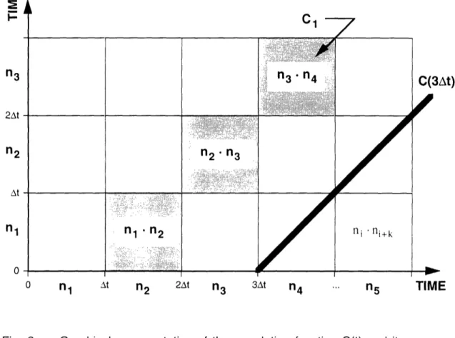
5

Fig. 2 Graphical representation of the correlation function C(t) and its approximation Ck. Each square's side represents the photon count in a corresponding interval. Thus the square itself represents the product of the sides' counts. The discrete approximation Ck is formed by the sum along a diagonal. The

continuous correlation function C(t) can be represented by a line.

n3 2At At n1 l 0 C(3At)

l

TIME n₁ At n2 2At 71

n

3 -"·C"3-"·IC"*l-rrrC *:' :··:·:·:·:i·i -·::·: -.vi_-.·,i ·-· ;.. ;jd:ii·"·'::_{i·;.:;.·--·:·-·;1 · .:·::··-··.···.·: :·:·:.::···}

n2'"3

',·'ll·'i·:i' ·· ,:·.·i·:· :::·::·::·j:·i::: -.j·:j:r·· .·.·;·i· ·:··::·, · ·-·- · · ·· ' :·

i

..-. . _ - .- ... _nl I i

n

2

ni

n2::

I l _

-1.2.3 Graphical Representation

Figure 2 shows a graphical representation of the construction of the correlation

function and its approximation. The horizontal and the vertical axes represent increasing time. Each segment (t, t+At] on either axis "holds" the photons collected during that interval, i.e., it represents

JI(t)

dt t

The area of each square in the plane represents the product of intensities "held" by its

sides. The squares of side At along each 45

°

_{line displaced k units from the origin}

correspond then to the products ni ni+k, thus their combined area represents the raw

correlation function Ck.

Clearly, as At --- 0, this approximates the continuous

correlation function C(t), so the continuous function corresponds simply to the 45° line displaced by a delay t from the origin.

The normalization of Gk becomes intuitively obvious in this scheme (see Figure

3). We have M squares distributed along a diagonal (dark gray) of a big square (lightly shaded). The sums in the denominator of Equation 3 correspond to the sides of this square (since each side "holds" all the photons in the interval of M units, thus corresponds to one of the sums). The diagonal has only M unit squares, while the shaded square has M2 of them. Thus for proper normalization we need to multiply the numerator by M.

1.2.4 Sources of Errors

The discrete correlation function is only an approximation. Let us consider the errors that can enter into this process. Even before the correlation function is computed, errors are introduced during the process of photodetection. The detector has only a finite

efficiency and not every photon produces a pulse. Furthermore, each detection is

followed by a dead time. Dead time means that if two photons arrive too close to each other, the second one will not be detected. This introduces a negative correlation at short

delay times. Finally, there is a probability of an afterpulse - one photon can trigger

several pulses. 'This enhances the correlation at short delay times. The errors of interest here are due to the discretization process itself. They are discussed below.

M -- ~~~~~~~~~~~~~~~~~~n M 2 1 0 M

li- ni

0 1 2 ... k IM k+M

.i=l

n+k

Fig. 3 Graphical illustration of the correlation function's normalization. The dark squares represent the raw correlation Ck. The sides of the lightly shaded square represent the intensity sums So and Sk. This square is then their product. Its area is M times bigger than the diagonal's. As the normalized correlation function has to be

dimensionless, it is formed as Gk=M.Ck/So.Sk.

1.2.4.1 Decimation

Standard implementation of a correlator uses registers to hold the delayed values of ni. The registers have a limited size, usually 4 (or 8) bits. Thus if the count rate exceeds 16 (or 256) counts per channel width the data has to be decimated (for example by throwing away every second pulse), which decreases the accuracy. In this scheme the

multiplication is replaced by repeated addition each time a new photon arrives, thus there

is no further error introduced from that direction. Hence these correlators are called 4*N

or 8*N. In the correlator described here each ni is stored in a 32 bit buffer, so one would

need to register more than 4109 counts per channel width to experience an overflow.

Thus the discrete correlation can be computed losslessly.

F:

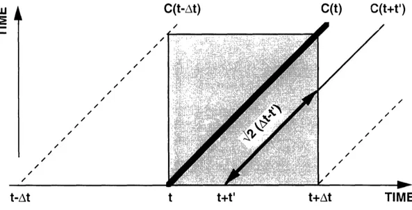
t-At t t+t' t+At TIME

Fig. 4 Construction for estimating the difference between the continuous correlation function C(t) and the discrete approximation Ct/At. The discrete approximation (the square) can be evaluated by integrating the diagonals (C(t+t')) weighted by the length of their intersection with the square (the arrows). The times between t-At

and t+At have to be considered (dashed lines).

1.2.4.2 Discretization

Let's examine the error introduced by the discrete approximation. As explained

above, in our graphical representation discrete correlation is represented by the sum of all tiles on one diagonal. Figure 4 shows the construction for evaluating the approximate

(discrete) correlation function from continuous ones (given some simplifying

assumptions, e.g., that the correlation function does not change in time). As before, the

45

°

diagonals represent the true (continuous) correlation function values at times

corresponding to their intersection with the lower edge, whereas the square represents the

approximate (discrete) value C(t)-Ck=t,,At and is the average of different C(t)'s

intersecting it. We compute it by summing the upper and the lower triangles:

CI(t)

=

At

)

t

t

(t)

f C(t t'). 2 (At-t'

d

C(t+t'

/2

(At-t)--0~~~~~~~~i0

~I·

· · \ Al·\ 1 Al· ·.

LLJ

At

- f

(C(t- t') + C(t + t')) (At- t'). dt'

We can get some idea about the magnitude of the difference C(t) - C(t) by expanding

C(t) in a Taylor series:

C(t+6t) = C(t) + C'(t)- t +

C"(t)

t

2

_+..

Plugging this in we obtain

At

C(t) =

t,

f(2 C(t)

0

= C(t) + C"(t)

.At

2 _{/ 12}

Thus the difference is directly related to the curvature. If the function does not bend too much within the period At, the accuracy should be good. A more illustrative example is

to look at a typical homodyne correlation function of the form C(t) = e

- 2

t/l. Plugging

it in we obtain At

f

f (C(t-t')+C(t

+t'))-(At-t')

dt'

At O 0 At

C(t)

= At2

[e2t-t)/

+ e-2(t+t')/z].(At-t') dt'

0 At

et/

1

1

2 cosh(2t'/'I)(At-t')dt'

0

-

C(t).

t-

.sinh2 ( t )

So

the

depends only on the quantity r =

ratio

C(t)/

C(t)

So the ratio C(t) / C(t) depends only on the quantity r = At / and equals

C(t) / C(t)

= sinh r 2

r

which for small r is very close to 1. In fact, the expansion about 0 gives

C(t)/C(t)

= 1 + 3T + --5 +

so even for r=0.1 the deviation is only 0.3%. Thus it is important to keep the channel width At small compared to time scales involved in the problem.

1.2.4.3 Finite Collection Time

Another source of errors arises from the finite collection time. This is especially

true for the large width channels. For example, a channel of lOs width is updated only once every 10s. Thus for a one minute run it will be updated at most 6 times (less in reality, since there is also a delay time before the channel is first accessed). The errors

introduced by finite collection time are reduced by using symmetric normalization

introduced by Schitzel et al. (3). This is nothing else than normalization with SO'Sk

rather than with (So)

2

, which would be easier from the technical point of view (because

less information needs to be kept track of). Reader is referred to (3) for a thorough analysis of finite collection time errors with and without symmetric normalization.

1.3 SOFTWARE DESIGN

The correlator described here is implemented mostly in software (except for the hardware that counts the incoming pulses and transfers them to computer's memory).

1.3.1 Why Logarithmic?

Computational power necessary to calculate the correlation function is related to

the number of squares (see Figure 1) composing the correlation function. Each square

represents one multiplication and one addition. Thus the required number of operations

per unit time is directly proportional to the number of channels (as each channel must be computed separately), but inversely proportional to the square side (At). Doubling the channel width At halves the number of squares per unit time hence halving the number of operations required to compute that channel. This fact, along with a property of the sum of a geometric series of the powers of 2, allows for a construction of a correlator in which

the channel width is doubled every several channels. The design described here uses

blocks of 8 channels. So if the width of channels 1 to 8 is 0ls, channels 9 to 16 have a width of 20gs, channels 17 to 24 - 40is, 25 to 32 - 8011s, etc. Thus if n instructions per

second are needed for the channels of the first block, n/2 are needed for the second, n/4

for the third, n/8 for the fourth, etc. The sum of such a geometric series converges:

n n n

n + - + - + - +... = 2n

2 4 8

Thus the total required computing power, even for an infinite number of channels, is

equal to that needed for two linear blocks.

1.3.2 Principle of Operation

For the sake of simplicity in the following discussion it will be assumed that each of the blocks has only four (rather than 8) channels. The graphical representation of the

logarithmic correlation process is presented in Figure 5.

The data structures needed to hold all the necessary information for computing the

correlation function are described below. To better reflect this computation, the indices

in the Equation 2 can be rewritten as:

M+k

Ck = A niik (5)

i=k+l

This demonstrates that to calculate Ck in real time we need to keep track of k past values of ni. This is implemented using a shift register - an entity where during each cycle the new data comes in on one side and the old data is pushed out on the other. There is one cell (from now on referred to as nk) for each channel of the block. The last two values pushed out are added together in a "limbo" and subsequently fed into the shift register of

the next block, reflecting the fact that the next block doubles the channel width. Of

course shifting of this higher block will be only half as frequent as that of the lower one (that is why we need the "limbo" to hold the intermediate value). N.B. the presence of the "limbo" corresponds to the white squares in Figure 5 where no correlation is collected

between the blocks.

Another structure is needed to hold the currently arriving data. Again. the

problem is complicated by the fact that each block doubles the channel width, so we need a separate no register (as it will be subsequently referred to) for each block. Analogously

to the nk case, two consecutive values from one block's no register are added together and

placed into next block's n register reflecting the fact that the next block's channels are

two times wider.

Next we need a way of keeping track of the sums So and Sk (defined in Equation

4) which occur in the denominator of Equation 3. In this implementation each channel

starts collecting data at a different time, so each of the sums for each of the channels runs

over a different set of numbers. This forces us to keep two sets of registers for each

channel (that's why the symmetric normalization is more difficult to implement). In

practice, only one register per block is being updated for each sum (as opposed to one per channel). The correction for each channel is pre-computed and stored separately.

Finally we need to keep track of the number of cycles (M) for each channel

(different for each one of them). This can be deduced from the total number of steps taken and thus only one number needs to be kept.

A.. 17 I.!

F-t

EL_

.+

r

7

17 m717

f

_:·· _e .

Fig. 5 Schematic representation of the logarithmic correlation. Course graining is introduced here by doubling the channel width every four channels (marked by different shades of gray). The number of computations per unit time (each square represents one computation) is halved by this operation. Since the sum of powers

of 1/,'2 is twice the first term, the total computing power required is

just twice that needed for the first four channels.

7

F_

F.

: : .. .

L:,...

..

o

_

,

-oo" .... ·· "t.:· ··

~

. ::. _. I....' !t :.. :. .... iI i

7

... ... ., He X .E

E

_

_ _

_{__}

:::.:::,:- _{i·:·:.·;::: .·i:·I·'·X:.:i:'i}...-..-:::::, "·''·:'·;' ';b··::.:i '' :.i· i. ·- · ·

:·;·:::·::··;;·-.-.·.···:

_{"P:·j:·: ·· ·:·i·rj}

.:.:il·'b"l:

·:·:··;.i·.·i·_: ·· · · ::·it:'l jrgs iiili:ZI:·i;l ::.,·.?::··:···:: :'::' ':'':"'_"'';' "';'" ···L·:'· i ';·:·'·:··: ·il:' :'· :'·:::::l::i: ':''' " '' ···"· '' ,71 .. :'·'.. '-··-····`'i'i·; · T:.'. · · :···: ·;··1 ::19·::1 *l*rc*rrrvki :·-.:·.·:·: i·::i:::._. ...·: :·-::::::.I::·:;:: ·.··

::·:· :.:... :·.···':::-·:i .-.:i-···:·ii.::':·:I·-d :..'.; _{- ·::-·} :···:-·:·:·:·::.r:i_{..:.·.:.8:':"i·'}:··:·

.. ·.:···- ·:i.P::.:i : :·:i· i li·-· i$i:

r··:ii:·,··,.·i · ·i i':14il '·:·.·iP.· _::: :::B:::j··:·l·-YI ·-·_i·::

· a:::·:; . ··:i·· :';·';I ·' ;;''":··-· ··-·· :·.i ::i'K:!:·''·:· ..:: ..i- i·;s ··· · ·'·: .; i_:··--,:::;:·<sub>'.''`::·: :· i:i-::'i.r:··r·i····</sub> i8,lalg i··,·i·i-;·i·:· ;.-:;-:·;···j·;·I i :i··i·:l::·i:i·iiOEa:::i! 8·i ·:*·· ·%n · ':i :··:::::·:···· ::BiIiP: ':':' ''"··": :.;i':!·:.·'·':'':":'":':''"""'" :.:·:::·:·.·.···::) i:·i:: :9i5' jj:" ·.-· · · ·:·::· - · ::·: :·:··::I':.:. ···:·:·::-··::·, i:-'::.sP.: :··: 6v,·''<sub>:'·-"</sub> ::I-·:·f· ·:-:i·r··::·:r .·:·.:.:.:j: :., <sub>··</sub> :...,. :·:·:·-: .:··· ::· :B':··:;;·· i i-·i.-·l·: . .-...·. · :... i·81··-· :::ii···i·l:: :·I:·-i-··::.:·i:·i·-··· : ····;· · iiiii·ii I"B';ii ::· ·:i·i.·`-' ·· :·j _{'''i·.··-·} ":' "" ·· :::·i:i ::··.·r,:-·:. .-·;·;_:. . :··i ::::; _·''' :.:I:i: ·i·.:. -;.i·;-·:··_··:·:..:· ·:···:; i··· .i-·j-9:.·.i.·. i··:· :*i:::::.:.·;i:i ::::'' :-::;.-::::::· ·: '8'i:.i:i:'i' .':::::: I:;·:.i.i :· ·· ··· -i·4:·`'<sub>·:·'i·i·,:·:· ::·</sub> :i··:·l:·:·--·-<sub>·-·</sub> :·: i:- ·- . ::· : ··· · -cl-:···· ··- .: .:·: ·-:I:- ·i::i:i: ;:i ··· : ·:':·':- :··; ·:::·;-::·: '"·':: ·:·:-::i···i·:-·i::';1::3· .·ij ''-···'·-···: :':.i·l·lj·r·r rrr*rrr*rm* '. iii :.:i::::i ·,I r:··:·:·::·i.: ;. ·· ···:·":·:: - ·.··.: .:·.i -·;.L;,-'··· ··· .-:.. :····:· i·:·i·: :·,····;···:: *iic ··· :·` i··:·._:i ·· ";''