Educational hardware for feedback systems

Educational Hardware for Feedback Systems

by

Isaac Dancy

Submitted to the Department of Electrical Engineering and Computer

Science

in partial fulfillment of the requirements for the degree of

Master of Engineering in Electrical Engineering and Computer Science

at the

MASSACHUSETTS INSTITUTE OF TECHNOLOGY

September 2004

@

Massachusetts Institute of Technology 2004. All rights reserved.

OF ECHtOLOGY

Author ...

UBRARIES

Department of Electrical Engineering and ompu

September 8, 2004

Dr. Kent undberg

Post-Docto

Lecturer

Thesis Supervisor

Accepted by...

...

Arthur C. Smith

Chairman, Department Committee on Graduate Students

Educational Hardware for Feedback Systems

by

Isaac Dancy

Submitted to the Department of Electrical Engineering and Computer Science on September 8, 2004, in partial fulfillment of the

requirements for the degree of

Master of Engineering in Electrical Engineering and Computer Science

Abstract

This thesis explores a variety of educational feedback systems with an emphasis on de-veloping them for in-class demonstrations and in-depth student projects. The nature of feedback systems means there is never a shortage of demonstrations or assignments that can truly capture the students' imagination and enthusiasm for class material. Unfortunately, it is sometimes the case that the feedback systems with the most potential for greatness are also unreliable, inaccurate, and inconsistent.

This thesis attempts to narrow the gap by exploring, analyzing, and building a variety of exciting feedback systems. A comparison of general-purpose and high-performance operational amplifiers is created. Hardware for a web-based laboratory on canonical second-order systems is implemented. Cheap magnetic levitation kits for in-term projects are made even cheaper. And finally, the inverted pendulum - a decades-old Course VI heirloom and featured demonstration - is restored to its past glory.

Thesis Supervisor: Dr. Kent Lundberg Title: Post-Doctoral Lecturer

Acknowledgments

A special thanks to Marita, Jacob, Zos, Leah, Ada, Mira, Anthony, Jesse, Leigh,

Abram, Mike and Cora. You never do see it written in that order. I'll leave the second generation of Dancy names for the next thesis acknowledgement.

I would also like to acknowledge those in the the field who inspire a passion for electrical engineering, including Ron Roscoe, Professor J. K. Roberge and those savvy SynQor engineers. Additionally, I could have never completed this project without the unconditional support and assistance of my advisor, Dr. Kent Lundberg.

Thanks to my parents for always pushing me to do my very honest best, even if I still won't smile for a post-strikeout photo-op.

And of course I need to thank Jenna soon-to-be-Dancy, who handled my thesis burden in her typically beautiful and graceful way.

Contents

1 Externally Compensated Operational Amplifier System 1.1 Introduction . . . . 1.2 Analysis . . . . 1.3 Design . . . . 1.3.1 Reduced-Gain Compensation 1.3.2 Lag Compensation . . . . . 1.4 Results . . . . 1.5 Future Work . . . . 1.6 Conclusion . . . .

2 Web-Based Second-Order Systems L

2.1 2.2 2.3 2.4 2.5 2.6 2.7 Introduction . . . . . Analysis . . . . . Hardware Interface . . . . Design . . . . . 2.4.1 Voltage-Controlled 2.4.2 Voltage-Controlled 2.4.3 Final Circuit . . . Results . . . . . Future Work . . . . . Conclusion . . . . . Integrator Gain Element 7 9 aboratory 9 10 12 12 14 15 16 17 19 19 20 21 22 22 23 23 24 27 28

3 Magnetic Levitation System 3.1 Introduction . . . . 3.2 Analysis . . . . 3.3 Design . . . . 3.4 Results . . . . 3.5 Future Work . . . . 3.6 Conclusions . . . .

4 Inverted Pendulum System

4.1 Introduction . . . . 4.2 Analysis . . . . 4.2.1 Inverted Pendulum System . 4.2.2 Motor Drive . . . . 4.2.3 Angle Sense . . . . 4.2.4 Position Sense . . . . 4.2.5 Final System Model . . . .

4.3 Design . . . . 4.3.1 Optical Encoder Design . . 4.3.2 Pendulum Controller . . . .

4.3.3 Former Pendulum Controller

4.4 Results . . . . 4.5 Future Work . . . . 4.6 Conclusions . . . .

A Weblab Assignment

B Pole-Zero Java Applet Assignment

C Magnetic Levitation Assignment

Modifications

D New Inverted Pendulum Schematic and Power-Up Procedure E Former Inverted Pendulum Schematic and Power-Up Procedure

29 . . . . 29 . . . . 30 . . . . 31 . . . . .. 32 . . . . 32 . . . . 34 35 . . . . 35 . . . 36 . . . 36 . . . 37 39 . . . 39 . . . 40 . - - 41 . . . 41 . . . 43 . . . 53 . . . 55 . . . 55 . . . . 56 57 63 69 77 81

Chapter 1

Externally Compensated

Operational Amplifier System

1.1

Introduction

Many commercial operational amplifiers are compensated such that they will be stable regardless of what may be connected to their terminals. This conservative compen-sation approach - while certainly attractive to a wide range of users and pleasing to datasheet appearances - can lead to disappointing performance in many standard applications. Operational amplifiers designed for advanced users and specific appli-cations can outperform general-purpose amplifiers whose goal is simply to work, but not to work well.

The OP27 and OP37 operational amplifiers by Analog Devices provide an excellent demonstration of this situation [1, 2]. The OP27 is a general-purpose amplifier with pleasing all-around specifications and guaranteed stability for all gain configurations below its own open-loop gain. The OP37 is a similar product, but has been optimized for applications with gains greater than five and cannot guarantee the same stability as the OP27 for gains below five. The datasheets, however, reveal that the OP37 slews at a rate of 17 V/ps, while the OP27 slews nearly an order of magnitude behind at a very quaint and unimpressive 2.8 V/ps.

The OP37 dominantly outperforms the OP27, even within a related product line

R

VI-Figure 1-1: Inverting-gain-of-i amplifier.

and device family, because it is optimized for high slew rates and bandwidth, thereby sacrificing stability at lower closed-loop gains. This optimization means that the

OP27 and the OP37 are not completely compatible in common circuit configurations. If a user replaced an OP27 in an inverting-gain-of-two amplifier with an OP37, the

circuit will no longer operate correctly, and this observation is often to the surprise and bewilderment of the user making the change.

The OP37, however, really could work if the external system was designed properly. The motivation driving an opamp demonstration for feedback systems is to show how higher-performance parts can be used in applications where at first glance they appear to fail. Circuit designers with a broad knowledge of classical feedback can use simple, external compensation to fix the problems present in the unstable feedback loop. This demonstration will juxtapose two inverting followers; one circuit using the pedestrian OP27, and another externally compensated configuration using the much faster OP37. The increased transient performance of the OP37 will be striking, while stressing to students the not-so-subtle fact that careful measures are absolutely required to ensure stability.

1.2

Analysis

This demonstration focuses on the inverting-gain-of-I circuit, shown in Figure 1-1. To better understand the stability dynamics, the analysis must ignore the usual ideality approach taught in many introductory courses.

Figure 1-2: Inverting-gain-of-i block diagram.

vi -1 2 VO

Figure 1-3: Inverting-gain-of-1 unity-feedback block diagram.

Figure 1-2 illustrates the block diagram for this circuit and Figure 1-3 is the simplified, unity-feedback block diagram for the same system. Basic block diagram manipulation provides the simplification between Figures 1-2 and 1-3; that is, when pushing a multiplicative factor through a summing junction, the reciprocal appears at the output. Note in Figure 1-3 that the ideal input-output relation preceeds the feedback loop while the loop represents some dynamics with a final value of one. Another equally important (though often neglected) point is the fact that this amplifier reduces the loop gain by a factor of one-half, which seems nonintuitive for a closed-loop unity-gain amplifier. Alas, the gain-bandwidth product is deceiving in this application.

Nevertheless, a simple Bode analysis should be sufficient to predict the closed-loop behavior of the system. The advantage of a Bode analysis is that only the open-loop behavior is considered, thus avoiding any extraneous math where additional errors can occur. The open-loop frequency response of the augmented loop transmission is all that is required for a Bode analysis.

The phase margin of the OP27 circuit at the crossover frequency of A(s)/2 is approximately 900 at 5 MHz, as indicated by the OP27 datasheet and reproduced in

Figure 1-4. With an OP37, however, the phase margin at crossover is either close to

zero or nonexistent - the datasheet doesn't even reveal the phase at this open-loop

location. This omission is to be expected since Analog Devices do not guarantee

2 25 GAINT 15 10O MARGIN -5_{-- 70} a-F --FREQUENCY -Hz

TPC 18. Gain, Phase Shift vs. Frequency 80 100 120 140 160 w 1SO 200 2W0

Figure 1-4: OP27 open-loop frequency-response characteristic, as it appears in [1].

4

al -140

11111 so1 1

FREQUENCY -HR

TPC 18. Gain, Phase Shift vs. Frequency

Figure 1-5: OP37 open-loop frequency-response characteristic, as it appears in [2].

stability for closed-loop gains less than five, let alone 1.

Thus, the challenge put forth in this demonstration is to design an inverting-gain-of-1 amplifier using a single OP37 by reducing its loop gain by at least a factor of five, ensuring a large positive phase margin, and consequently, superior transient characteristic when compared to the OP27.

1.3

Design

1.3.1

Reduced-Gain Compensation

The OP37's problem is that its loop gain is greater than one when the phase drops rapidly. Closed-loop systems calling for higher gain will invariably have a loop

trans--2

R

R

VIc

RC

+

Figure 1-6: Reduced-gain amplifier configuration.

mission with less gain, meaning that stability is not a problem. A reduction of loop transmission can still be achieved without effecting closed-loop gain by adding a re-sistance at the inverting terminal of the operational amplifier. Figure 1-6 illustrates this configuration, implementing a form of reduced-gain compensation.

To develop the block diagram describing this configuration, it is necessary to solve for the voltage at the inverting input of the op amp. Superposition of v, and vo yields

RIIRc RIIRc (

R+ RIRc R+ RIIRc '

while the open-loop characteristic of the op amp determines

vo = -A(s)v-. (1.2)

These relations combine to develop a block diagram description of the amplifier (Fig-ure 1-7). Block diagram manipulation simplifies Fig(Fig-ure 1-7 into the unity-feedback configuration, shown in Figure 1-8. The ideal relation of this configuration is still a gain of -1, yet the loop gain has become

L~s) =RI|Rc

L(s) R IRC A(s). (1.3)

R + R|Rc

Therefore, if the quantity RIIRc/(R + RII Rc) is less than or equal to 1, then the

system has achieved at least 700 of phase margin while matching the low gain of the

OP27. The value of compensation resistor to ensure stability is 13

RL

RR+R||Rc

Figure 1-7: Reduced-gain amplifier block diagram.

Figure 1-8: Reduced-gain, unity-feedback amplifier block diagram.

1

Rc < -R. (1.4)

3

The reduced-gain compensation was implemented in this demonstration with R =

10 kQ and RC = 1.3 kQ, a reduced-gain compensation of 0.103.

1.3.2

Lag Compensation

One disadvantage of the compensation technique described in the previous section is the fact that it reduces the gain of the loop transmission over all frequencies, when it is only necessary near the crossover frequency. Reduced-gain compensation unnec-essarily decreases the DC gain of the open-loop, and thus degrades the steady-state error response of the closed-loop response. Lag compensation can replace reduced-gain compensation to maintain open-loop low frequency reduced-gain while also ensuring a safe crossover phase margin.

Lag compensation can he realized with a series Rag-C circuit applied instead of the reduced-gain resistor, Rc (shown in Figure 1-9). The impedance of the lag branch is

R

R

Rag

C

Figure 1-9: Lag compensation configuration.

_RiagCs +l

ZC(S) = . (1.5)

CS

To understand how the lag compensation will behave, simply substitute Zc(s) for

Rc in the reduced-gain equation. This substitution into Equation 1.3 yields the loop

gain characteristic for the lag-compensated configuration

L(s) = 1 (Riag~ s A(s). (1.6)

2(1 + Riag)Cs + 1

This implementation of lag compensation is not perfect, as there is still a one-half reduction of DC gain, but this fraction is still a vast improvement over the previous reduced-gain compensation of 0.103.

This lag compensation was implemented with R = 10 kQ, Riag = 560 Q, and

C = 259 pF.

1.4

Results

The OP27 inverting-gain-of-I circuit was built as well as a selectable reduced-gain, lag-compensated circuit built with an OP37. Both circuits were driven by a ring oscillator circuit which transitions faster than either opamp could possibly match,

El ChV _.4 12 Ch2L 2 00 __ 1. 0 s A| Ch1 2.4 4y

Ch3 .OO Ch3

2-....OV-(a) OP27 versus reduced-gain OP37. (b) OP27 versus lag-compensated OP37.

Figure 1-10: Measured Results. Top trace is the OP37 response, middle trace is the

OP27 response, and the bottom trace is the ring oscillator drive signal.

thus ensuring that both circuits will slew. A complete schematic can be found in Figure 1-11.

A comparison of the OP27 to the reduced-gain OP37 circuit is shown in Figure

1-10a, and a comparision with the lag-compensated OP37 follows in Figure 1-10b. It is clear in both cases that the OP37 configuration slews faster.

1.5

Future Work

While the demonstration convincingly illustrates the difference in slew rate between the OP27 and OP37, it would also be preferable that there be some way to illustrate the difference in steady-state error between the reduced-gain and lag compensation configurations. The error is expressed in the voltage present at the inverting terminal of the op amp, but unfortunately this voltage is too small to detect. This demonstra-tion would be enhanced if some means to display the error voltage of the OP37 were possible.

Furthermore, the response of the lag compensated response (Figure 1-10b) suggests less open-loop phase margin than the corresponding reduced-gain response The demo would be improved with a slight adjustment to the compensator such that a greater phase margin was achieved.

r 4.. ... ... __... ....... ...

...

7:

...

...

1.6

Conclusion

While it is often the goal of operational amplifier manufacturers to produce perfectly stable designs for any user application, this objective is clearly at the sacrifice of better transient behavior. With careful attention to detail, however, many discrete circuit designers can use higher-performance operational amplifiers for a wide range of applications, even if at first glance it appears they would not work.

If it does not work the first time, feedback makes it possible to try, try again.

a-0 LO L()

o

L-0+

(1)

Chapter

2

Web-Based Second-Order Systems

Laboratory

2.1

Introduction

The first order of semesterly business in many feedback courses is to re-awaken the students' familiarities with basic transfer functions and their behavior. This review is usually achieved with a barrage of pole-zero, step response, or Bode plot associa-tions in homework and a merciless rehashing of terms and definiassocia-tions in lectures or recitations - or both.

The motivation behind a web-based laboratory on second-order systems is to bypass the prominence and inherent boredom of these expository details and give students an interactive and engaging way to review material while simultaneously providing feedback to course staff with each students' individual degree of under-standing of reviewed material.

A "weblab" is a perfect way to achieve this. Weblabs consist of some software

front-end running experiments on one back-end device [3]. A weblab designed to

test and familiarize students with canonical second-order systems can help to quickly ready students with the more complicated and interesting matters at hand.

With a software interface already in place, all that remains is to build a set of hard-ware to communicate through the interface and accurately simulate the conditions

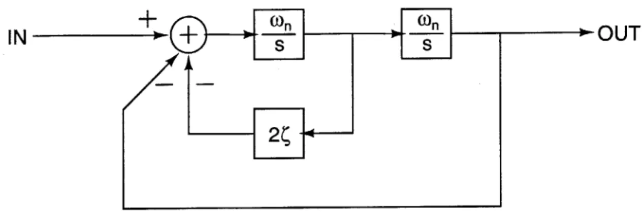
IN

-OUT

Figure 2-1: State-variable filter topology. Closed-loop transfer function implements the canonical second-order system, using only open-loop integrators and gain ele-ments.

under test [3, 4].

2.2

Analysis

This weblab requires hardware that implements a variety of second-order systems, from lightly damped conjugate pole pairs to over-damped, negative-real-axis poles. The parameters of these systems must also be user-settable via the lab server. To

achieve a greater range of systems and results, two canonical second-order systems will be cascaded, giving the user four exclusive degrees of freedom.

The experiment hardware must be either current- or voltage-controlled in order to translate lab server commands into second-order system parameters. The state-variable filter (block diagram shown in Figure 2-1) is a system which can provide such functionality. The basis of the state-variable filter is its dependence on feedback and simple building blocks such as integrators and gain elements.

The closed form of the state-variable filter is

W2

H(s) = + W2' (2.1)

s2 +2(Wns +w

which is exactly the canonical second-order transfer function. If parameters wo and ( are voltage-controlled, then this topology can implement any second-order frequency

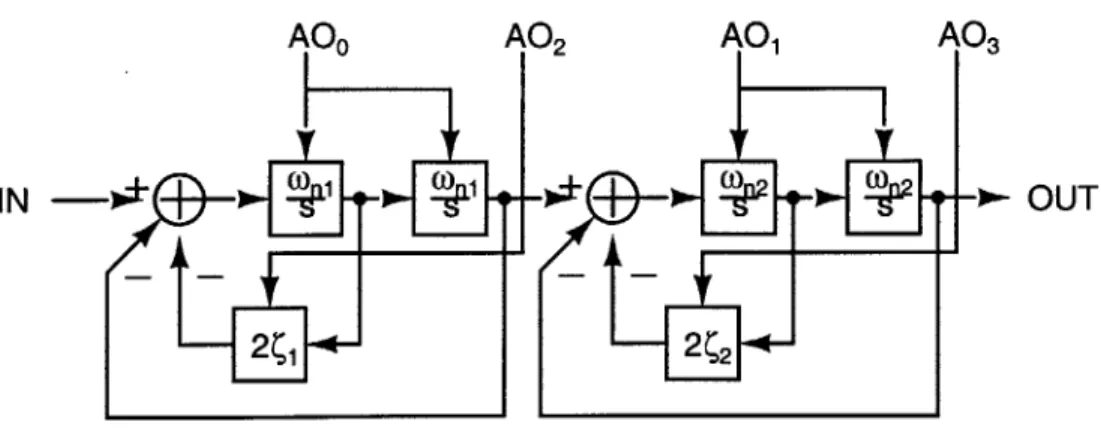
AOO A02 AO1 A03

2(1 2 2

Figure 2-2: Controlled and cascaded state-variable filter system. AO signals control the gain of connected system blocks. Cascade provides four user-settable system poles.

response. In fact, this topology is widely used in musical applications due to its broad synthesis capabilities [5, 6].

Thus, the state-variable filter uses simple integrators, gain elements, and feedback to implement a variety of second-order reponses. If the integrator and feedback gains are carefully controlled, then any desired response can be realized. Figure 2-2 represents the overall topology of this cascaded state-variable filter design. AO, are command signals expressed via the lab server through the hardware interface. A frequency analyzer controls IN and measures the response at OUT.

2.3

Hardware Interface

The lab server exists on location with the experiment hardware and communicates with the lab broker to receive all client experiment parameters [7]. The LabJackTM connects to the lab server through the universal serial bus (USB) and expresses the client commands for use by the experiment-specific hardware [8].

The LabJackTM drives two analog, 5-volt voltage signals and 20 lines of 5V TTL-compatible digital logic. These 20 lines are programmed into two 10-bit binary signals in the software, yielding a total of four command signals.

The digital signals require some processing before any voltage-controlled

Server

LabJack

4,

t

Figure 2-3: Server-side hardware configuration. Voltmeters provide administrators with the current command signals. Lab server controls the HP3562A measurement via the HPJB interface.

iment circuit can possibly make use of them. The processing is performed with separate hardware, which converts the two 10-bit digital command signals into 5-volt analog voltages. An overall diagram of the experiment setup is shown in Figure 2-3.

2.4

Design

The convenience of the state-variable filter design is the reliance on simple variable-gain function elements. The circuit design can focus simply on a variable-variable-gain integra-tor and implement the feedback topology with simple adder circuits and variable-gain blocks.

2.4.1

Voltage-Controlled Integrator

Often times transimpedance amplifiers form the basis of a variable-gain integrator when current is the command medium [9]. This topology, while correct, performs no better than the linearity of the transimpedance amplifier which implements it, and this specification can often times be limited.

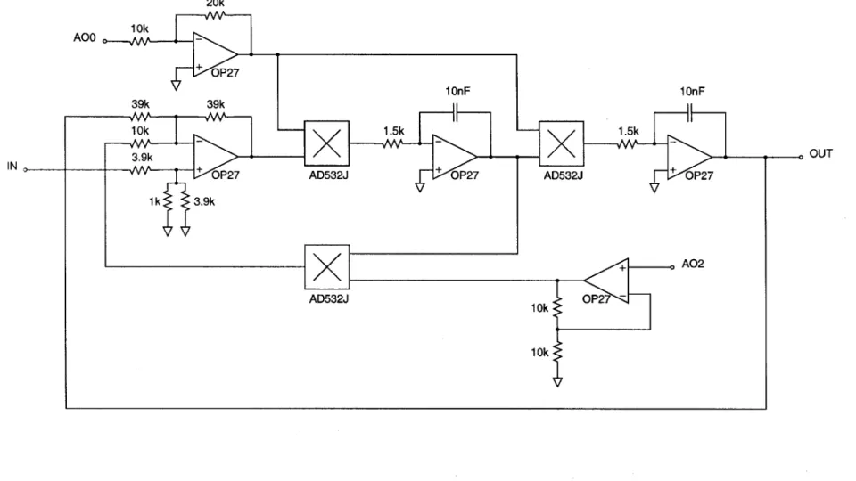
OUT2

OUT3

Vo

20k

AOo 10 10nF

+ P7 _1.5k

OUT

IN 0 AD532J 7

Figure 2-4: Voltage-controlled inverting integrator. Inverting-gain-of-2 amplifier scales A00,1 up to the full range of the AD532J and results in a total

noninvert-ing relation from IN to OUT.

Alternatively, a voltage command signal requires voltage multipliers and instead depends greatly on the linearity of voltage multipliers. Voltage multipliers with greater linearity can be found, though at a price exceeding $29 per chip [10]. For-tunately, Analog Devices generously donated the AD532 voltage multipliers used in this hardware, allowing the design to forego cost and proceed.

The circuit diagram for an inverting integrator is shown in Figure 2-4. The input-output relation for this circuit is

V1 = V) R

(2.2)

VI \= (-V } RCs'

where the voltage vc can be tuned to control the gain of the integrator.

2.4.2

Voltage-Controlled Gain Element

A voltage-controlled gain element can be implemented using another AD532 device,

where vc/10 V is the variable-gain parameter.

2.4.3

Final Circuit

These two simple building blocks are configured in the feedback topology to realize the state-variable filter. Two systems are cascaded together to realize a greater variety of systems and assignment possibilities. The 5-volt analog signals are multiplied by

two in order to utilize the full dynamic range of the AD532 chips. The two voltages controlling the w, parameters are also inverted to make the integrators noninverting in the open-loop. A final circuit schematic of the state-variable filter is illustrated in Figure 2-5. The complete system consists of two copies of this circuit.

2.5

Results

The total system was built and connected [11]. The system succeeds in producing smooth, accurate frequency responses and compares favorably to theoretical results. Figure 2-6 compares an experimental result to a theoretical result, and confirms this system's functionality.

Additionally, a laboratory assignment (Appendix A) has been written that actively engages students in a productive discovery or review of second-order system responses and parameters. Another assignment, while not based on the weblab itself, does serve to complement the laboratory and can be found in Appendix B.

Students will be expected to evaluate the state-variable filter topology in block diagram and circuit form, finding relations between the voltage command signals and the corresponding block diagram parameters. Students will then relate a sampling of second-order systems (Figures 2-7a and 2-7b), express these systems in order of their second-order parameters, then calculate the voltages required to make the experiment implement the systems.

While we hope that students will fine-tune their understanding of second-order systems, we also hope that they will make a few observations relating to the limitations of this specific design and implementation - problems inherent in any undertaking of this kind. For example, students should observe the difficulty in simulating the sharp and large-valued gains evident in low-damped systems. Students should also observe the difficulty in discerning between similar systems - i.e., four distinct, negative poles closely clustered versus four poles at one, single location.

Ultimately, students will rediscover and explore second-order systems while real-izing the minor issues inherent in the hardware's implementation.

I-0 CLC~ I + LO~ C\J 0 + a. C '\ Y0L~ LO z Figure 2-5: State-variable filter circuit implementation. Three multipliers per filter make this circuit expensive to build. 0\ I

10 3

Radians per Second i 10 . .. . . .. ... ... 6 . . . . ... . . . 0 - 1 0 ... .. ... ... .... ... ... - 2 0 ... ... ... .... .. CO - 3 0 ... .... .... ... ... ... % ... . - 4 0 . .. .... .. .. ... ... ... ... ... .... .... .. .... ... ... .... ... . Cc - 5 0 . ... ... .... .. ... - 6 0 . ... ... ... .... ... ... - 7 0 . .. .... 6 ... ... .. .. ... .. ... ... . .... ... .. ... .. .. ... ... .... .... .... ... ... ... . - 8 0 -... ... ...... -90 10 2 10 3 10

Radians per Second

. ... ... . . . . ... . . . . .... . . .... . . . ... ...... .... . ... . . ... . . . .. ... .... ..: -90 -180 (D Ca 0--270 10

j) ju XX

XX

(a) (b)

Figure 2-7: Example assignment systems.

2.6

Future Work

While the current hardware works well, there are some areas where future efforts should be directed. In specific, the experiment phase measurements are not perfectly ideal, and the system is limited by the dynamic range of the multiplier ICs.

The state-variable filter uses feedback loops to implement the various canonical second-order responses desired. The ideal results of these feedback loops do perfectly match the responses of the desired systems, but in practice the measurements are not ideal. This error stems from the operational amplifier's high-frequency, parasitic pole. This pole negatively affects the high-frequency performance of each integration, and compounds due to the four amplifiers present in the forward signal path. This non-ideality is most obvious upon careful inspection of the phase data. The multiple parasitic poles present additional negative phase several decades below the actual parasitic location.

Phase error can possibly improve with higher-performance operational amplifiers, but this solution is both costly and trivial - it is always the case that higher-performance parts can provide some relief. Another, more practical solution is the addition of lead compensators in series with the integrators. The lead compensation provides a positive phase "bump" at the geometric mean of the compensator. If the bump is placed near the location of the parasitic op-amp pole, then the measured

phase error should be improved.

Dynamic range should also be further investigated. The current system can only provide a linear range of w. and ( between 0 and 5 V. The resolution of the LabJackTM and the digital-to-analog converters means that practically the dynamic range of pos-sible values is no better than two decades. A logarithmic relationship between com-mand voltage and circuit parameters would enable a greater range of responses possi-ble, but likely expose the limits of saturation and frequency performance throughout the rest of the state-variable filter. In other words, proceed with caution.

2.7

Conclusion

Web-based laboratories are useful educational tools because they essentially provide a "control" with which to compare the knowledge of every student. Weblabs also streamline the students' learning process by allowing them to skip the tedious circuit tasks invovled with building a specific system, while still utilizing the actual, measured results from a real-world system.

Weblabs, however, are limited by the hardware which executes the experiment. While building customizable, settable systems is often possible, the dynamic range and practical performance of such circuits can sometimes cause problems.

For the purposes of this experiment, however, the state-variable filter does prove to be robust, smooth and an all-around worthy solution. While possibilities do exist which can expand its functional range and improve its system model, the current system will go into immediate use and hopefully save future students the continued trauma of boring start-of-term review.

Chapter 3

Magnetic Levitation System

3.1

Introduction

Magnetic levitation is an often-used demonstration for feedback systems courses due to its challenging open-loop instabilities and impressive closed-loop behavior. Lev-itation systems are both difficult to build and expensive to assemble. The systems require a coil to generate an upward magnetic field, an object for levitation, and a position sensor.

In many class demonstrations the position sense is achieved with a light bulb and photodiode. The closed-loop system controls the position of the levitated object to some fixed intensity of light at the photodiode - as the object moves closer to the coil, light intensity decreases, while if the object moves away from the coil, the light intensity increases. This position sensor provides the necessary information to provide the overall system with negative feedback.

This setup, however, is too expensive and elaborate for many students to build on their own for a class project. To meet the requirements of cheaper cost and less overall complexity, a unique and different kit must be assembled.

A new magnetic levitation kit for students has been recently developed that uses

a Hall-Effect sensor and H-bridge circuitry to bring the cost down to less than $20 [12, 13]. The Hall-Effect sensor detects the present magnetic field, and can therefore provide some sense on the position of a levitated object with a permanent magnet

attached.

This system is not without its own drawbacks, however. The sensor is corrupted

by the magnetic field generated by the coil, making stable behavior a very

initial-condition dependent endeavor. Furthermore, the H-bridge circuitry, while simple for students to configure, is a large portion of the $20-kit cost. Students often attain stability with a varible-gain in the sensor's feedback loop, as well as painstaking trial-and-error routines concerning the size and weight of levitated objects.

This chapter will explore the possibilities of improving this current system with better position sense and cheaper power electronics. Slight modifications and ap-proaches will result in a final kit cost closer to $10, and another interesting result.

3.2

Analysis

Magnetic levitation derivations are not difficult to find, and they reveal a very ex-pected result [14]. The levitation system consists of a right-half-plane zero and a left-half-plane-zero distributed evenly on either side of the origin. The pole locations are dependent on the mass of the levitated object, the necessary DC coil current necessary for equilibrium, and the distance below the coil the object will levitate. This result is not particularly useful in the construction of cheap magnetic levitation kits because some parameters are difficult to determine, and for the cost spent it is difficult to find parts with reliable characteristics. Furthermore, most demo systems are not concerned with transient behavior or dynamic range; they are simply designed to work for one standard setup [14].

One practical solution to this analysis issue, and something that has already been implemented by many students and encouraged by course staff, is to build the basic system and use measurements of the closed-loop system to determine what compen-sation is necessary to stabilize the system. Basic root locus reveals that in a feedback loop the two poles will meet at the origin and travel along the jw-axis. This closed-loop system is not stable, but should be marginally stable enough to allow students to measure the damping frequency of the closed-loop response.

Root Locus 25 20- 15- 10-CU 00 .. . . . .. . . . -10- -15- -20--25 -10 -8 -6 -4 -2 0 2 Real Axis

Figure 3-1: Example root-locus of magnetic levitation system with series lead com-pensation. Lead compensation uses conservation of centroid to stabilize conjugate pair.

With this information students are able to design a lead compensator to improve the stability of the system. The lead compensator moves the centroid into the left-half plane and thus pulls the two system poles into a stable region. An example of this root locus is illustrated in Figure 3-1.

3.3

Design

The $10 levitation kit was compensated in a similar manner as the previous versions, with a variable gain amplifier in series with the Hall-Effect sensor and a lead

com-pensator, which drives the Micrel fan chip. The kits differ from the previous version,

however, because the fan chip now merely drives a simple transistor configured to

drive current through the electroinagnetic coil, thus eliminating the costly H-bridge

circuits. This power drive approach was first suggested by [15, 16]. Figure 3-2 illus-trates the modified controller circuitry which incorporates the new power electronic scheme.

This plug-and-play solution is viable because the Micrel fan chip is actually opti-mized to drive transistors.

3.4

Results

A levitation system was built and tested as described, with a final kit cost of $10.

Additionally, with proper attention to the loop gain of the system, the kit is capable of suspending objects without a permanent magnet attached. This capability is a subtle side-effect of the Hall-Effect sensor. The proximity of a metal object beneath the coil actually effects the number of magnetic field lines passing through the sensor, and therefore the sensor provides a small amount of feedback even without a magnet present. A controller system with high enough loop gain can therefore levitate metal objects without needing permanent magnets.

3.5

Future Work

While the Hall-Effect sensor remains one of the keys to a cheap levitation system, its difficult and nonlinear behavior remains a big obstacle for the realization of bet-ter stability and general levitating behavior. Future work in cheap levitation should include a thorough investigation of the true behavior of this sensor. A totally au-tomated system could be achieved if an understanding of the nature of the position sense existed. Future work could include a proper modeling and linearization of the Hall-Effect sensor.

I \\\\\\\\\\\\\

Lq

3.6

Conclusions

Cheap magnetic levitation can be achieved similar to previous kits with the addition of a single transistor coil drive. Further, the need for permanent magnets can be negated with careful attention paid to feedback-loop gain.

Chapter 4

Inverted Pendulum System

4.1

Introduction

The stabilization of the inverted-pendulum system, illustrated in Figure 4-1, is an often-used demonstration in many control and feedback systems courses. At MIT, the inverted-pendulum demonstration is a traditional favorite amongst students, while recently developing into a headache for department staff that worsens in intensity and duration with each passing semester. The inverted-pendulum now exists as a phan-tom, making appearances in lecture and working tenuously while reserved lecturers force a smile, or appearing in lecture but being quickly abandoned to the corner of the hall while teased students take notes and wonder when or if the demo is going to be shown.

The demonstration can be made to work for a few moments, but no longer contin-uously. The demonstration can be having a "good day," but the sensors for pendulum angle or cart postion may fail at any moment and without warning or provocation.

The fact that the schematic is not shown to students is not to maintain some department or trade secret, but rather as a safety measure to preserve what students have already learned. The truth is nobody really knows why or how the systems works while it is behaving, and certainly nobody knows the reason when it fails. For a long time the system just plain worked, and this bottom line combined with its recent deterioration has quickly made it the prodigal son of the MIT Electrical Engineering

0x

Figure 4-1: Inverted-pendulum system. Motor drives right-hand-side pulley and po-sition sense mounts on the left-hand-side pulley. Track length and pendulum length are 1.75 meters and 0.40 meters, respectively.

and Computer Science department.

This chapter will review the analysis of the system, implement new sensors for angle and position, and attempt to rebuild the control with a well-known solution that can restore the department's inverted-pendulum system to its past glory and once robust behavior.

4.2

Analysis

4.2.1

Inverted Pendulum System

The inverted pendulum demonstration is similar to what is pictured in Figure 4-1. The total track length is 1.75 meters, and the cart is driven by a motor which drives the right-hand-side pulley. Braided cord connects to either end of the cart and around the driven pulley and the free-spinning pulley. A position sensor is placed on the axle of the free-spinning pulley, and an angle sense is placed at the hinge of the inverted pendulum.

Using the parameter and sign definitions from Figure 4-1, the angular acceleration of the pendulum is equal to (g/l) sin 0, while a cart acceleration of t generates an angular acceleration of -(z/1) cos 0. These relations can be combined and linearized to generate a simple, linear model of the system for small perturbations in 0.

0 = (g/l) sin 0 - (z/l) cos 9.

The presence of the trigonometric functions sine and cosine in Equation 4.1 mean that this differential equation is not linear. Assuming, however, that the pendulum angle will always be nearly zero, the small-angle approximations can be substituted to yield a linear differential equation. For small 9, sin 9 ~ 0 and cos 9 ~ 1, yielding the linear equation

6

Taking the Laplace Transform of this linear differential equation generates the system transfer function G(s), describing the small-signal response of pendulum angle for small-signal changes in cart position

s

where TL =

l/g.

TL = 0.2 s. (g/l)E(s) -

s

pendulum is approximately 40 cm, making

4.2.2

Motor Drive

The cart will be driven by a DC motor via two pulleys and a braided cord. The braided cord is secured to both sides of the cart and is wrapped around both the free-wheel pulley and the motor-driven pulley. The specific motor transfer function, relating input voltage to output shaft angle, is

37

Pole-Zero Map 0.8 0.6 0.4 0.2 a ... 0 . .. .x... x . ... . . .. .. .. E -0.2 --0.4 - -0.8--20 -15 -10 -5 0 5 10 15 20 Real Axia

Figure 4-2: Pole-zero plot of G(s)M(s). Two zeroes at the origin create difficult locus trajectories for right-half-plane poles.

M (S) = motor 4.87 [radi (47)

V(s) s(0.066s + 1) [VJ

The angle-to-position coefficient, 1/n, as well as the tachometer coefficient, kTACH, are measured as 1 Fml - = 0.0318 (4.8) n rad] and

.[vi

These functions lead to an open-loop system characterized by the pole-zero plot in Figure 4-2. The right-half-plane pole as well as the two zeroes at the origin make this compensation a particularly unique challenge. This system is both open-loop and closed-loop unstable.

4.2.3

Angle Sense

The new angle measurement for the inverted pendulum will be produced by a continuous-turn servo-potentiometer mounted at the inverted pendulum's hinge. The poten-tiometer is set such that a vertical pendulum produces 0 volts, while positive angles produce a negative voltage proportional to the supply voltage. Since the pendulum can swing a maximum of 7r radians, this angle sense can utilize half of the power

sup-ply range. The old system setup used a 10-turn potentiometer at the same location,

meaning that it only used one-twentieth of the full range. With a supply voltage of 15 volts, the angle coefficient is

K = -4.77

[-

Note the negative sign of KO; this polarity is due to definition of the system and implementation of the sensor. Most likely, the original system called for -0, and this reversal is an easy way to avoid an additional inverting amplifier in the controller.

4.2.4

Position Sense

A 10-turn trim potentiometer was also used in the old system's position sense. In

general, trim potentiometers are not meant for servo applications, and therefore the potentiometer can fail during continuous use due to internal contact failures.

Since the potentiometer is mounted to the free-spinning pulley opposite the motor - and is, therefore, coupled to position via the angle-to-position coefficient of Equa-tion 4.8 - a similar continuous-turn servo-potentiometer cannot be used to sense position since several rotations are required as the cart moves from one end of the track to the other.

One solution is to use an extra gear which down-samples the free-wheel pulley ro-tations and places the servo-potentiometer on the extra gear. This solution, however,

is costly and requires the kind of mechanical expertise and time that Course VI staff are unable to provide and maintain.

An electrical solution is to use an optical encoder, which is a digital sensor that

produces pulses proportional to pulley rotations. An encoder can be chosen with the correct pulse rating to simulate the effect of down-sampling.

While the design of the encoder circuitry will be explained later, enough informa-tion already exists to determine the posiinforma-tion sensor coefficient. The encoder chosen produces 256 pulses per one revolution of the free-wheel pulley. A 12-bit binary counter counts these pulses and a digital-to-analog converter produces a +10-volt output. The total output swing of the DAC is therefore

__ [radi 256 ~bits] +10 [Vi

1 x --- X 212 x 1.75 [ m] = +5.5 V, (4.11)

0.0318 m 2-7 r rad 21 bits

where the total length of the track is 1.75 meters. Since the output swings only +5.5 volts from the center of the track to the endpoints, the output is doubled with a separate LF411 amplifier, leading to a final position coefficient of

Kx = 12.6 . (4.12)

Since the track spans 0.875 meters from the center to the endpoints, this means that the position sensor will generate an analog voltage that swings ±11 volts from center to end.

4.2.5

Final System Model

With the pendubim system, motor drive and sensors completely analyzed, Figure 4-3 illustrates the entire open-loop system. Coefficients with an "M" subscript indicate a parameter measurement, and are thus a, voltage.

V 0.066s+1 + .. 1- +--+

0M

TACH-4+ 0.16 --- 4.77

XM 12.6

Figure 4-3: Complete inverted pendulum open-loop system. "M" subscript denotes a voltage measurement of the system parameter. Natural integration occurs between motor shaft speed and motor shaft angle.

4.3

Design

4.3.1

Optical Encoder Design

Since feedback systems courses are mostly taught using analog systems and analog electronics, the most important aspect of the optical encoder design - a digital system - is that it functions reliably and without attracting attention to itself. The encoder should simply provide a voltage proportional to the position of the cart on the track, and nothing more.

Of course, since this sensor is digital its output will not be continuous, but rather

a staircase of voltage where step-size relates to the resolution of the system. As mentioned before, the encoder divides the track into 2242 equally-sized pieces (1281 bits per meter). The track length is 175 cm, so the resolution of a 256-pulse encoder is 781 pm. This step-size should be sufficient for the controller.

As shown in Figure 4-4, the topology of the sensor includes the encoder, a

quadra-ture detector, a 12-bit counter, and a digital-to-analog converter. The optical encoder

outputs two signals in quadrature; meaning that one signal leads the other by 900

Optical Quadrature

Encoder Detector Counter DAC

A _UPVOUT CTB DOWN vu 001100101001 -6.044V CW--- 001100101010 -> -6.039V S0100-6.044V

Cw

Figure 4-4: Optical encoder sense diagram. Encoder controls two signals in quadra-ture, which are decoded into UP/DOWN pulses and counted with 12 bits before analog conversion.

during clockwise revolutions, while the opposite is true for counter-clockwise revolu-tions. The quadrature detector senses the direction of movement, and controls two signals, sending pulses on the UP line while the encoder rotates clockwise (in the positive x direction), or sending pulses on the DOWN line while the encoder rotates counter-clockwise (and in the negative x direction). A 12-bit up/down counter is a standard part found in most digital logic families which counts from 0 to 4095. The counter should be initialized to 2047 so that it counts equally up and down from the center point of the track. This initialization means the cart must be centered during power-up to properly configure the counters. The digital-to-analog converter converts the counter output into an analog voltage, which is sent to the controller as the analog measurement.

This circuitry is implemented using the standard SN74LS family of digital products (Figure 4-5). The AD767 by Analog Devices serves as the 12-bit digital-to-analog converter, and is configured to offset the output so the middle of the track corresponds to ground, while the ends of the track correspond to +11 V.

The circuitry sufficiently substitutes for the old 10-turn potentiometer, and should survive the test of time; allowing instructors to now run the demonstration continu-ously and without fear that the contacts within the potentiometer will corrode and

fail at any time.

4.3.2

Pendulum Controller

Overview

The compensation approach demonstrated here reflects the theoretical solution an-nually taught in 6.302 Feedback Systems. This compensation methodically tackles the various difficulties inherent in stabilizing an inverted pendulum system.

The basic stability problem stems from the inverted pendulum system function derived in Equation 4.5 and repeated here in Equation 4.13:

e(s) =1 _ 2 -0.102s 2 _(4.13)

X(s) g rTs2 - 1 0.04s2 _ 1

This system introduces two zeroes at the origin and two poles distributed around the origin at s = ±5 rad/s. The zeroes are particularly difficult during compensation

be-cause in feedback closed-loop poles approach the open-loop zero locations. Therefore, the only way to "pull" the right-half-plane zero into the left-half-plane is to intro-duce a second unstable pole - otherwise the unstable pendulum pole would simply approach the origin from the right under feedback, and the system would never be stable.

Positive feedback around the motor moves its integration pole off the origin and into the right-half-plane; essentially, positive feedback means that the only equilib-rium point is a vertical pendulum at the center of the track. Otherwise, the system would stabilize the angle but run right off the end of the track. Further, the addition of a lag compensator with a low-frequency pole and a zero at s > 5 rad/s results in

the root-locus plot of Figure 4-6. This controller strategy is the exact compensation scheme proposed in feedback courses and is thus a "textbook" solution to the inverted pendulum problem. If an actual controller used this scheme, it would enhance the value of the approach's educational value.

The general block diagram which implements this feedback topology is illustrated in Figure 4-7. The controller design is performed from the inner-most loop to the

Optical Encoder 74LSOO +5 NAND -B1 B4 Y1 A4 A2 Y4 --B2 B3 --Y2 A3 -GD Y3 74LS86 +5 XOR Al Vc0 B1 B4 Y1 A4 A2 Y4 20k 20k Y2 A3 GND Y3 74LS107N +5 0 CLR - -OCLR, IQ 1CLK - --1K 2K 20 2CLR --- OCLR, 20 2CLK GND 2J Pendulum Controller 15 0 i. +15 7 2 6 _LF411 3 4 -15 47N DN +15-15 0-UP o0 v -15 +15 7 ~ 1pF 0.1p 1 F 0.11

7!77!7

TITT

UP/DOWN Counter UP/DOWN Counter UP

--B Vce ,:I B LJVcc C* B, 0-- QB A 8,0O- %s A B, 0-Bo 0-- GA CL B, 0- , CL B, 0-DOWN --- DOWN UP -- - -- - UP CO B2 0-- Q0 LOAD ---- Be -- Qr LOAD B, 0 -B3 0- 0 C B? 0- QD C B,, 0-GND D 4t _GND D 1M 7805 +5 Vcc GND +5 +15 - '.F- -0.33ptF 1 ₂ 3 + 1gpF 0.1~ 11f F .pF All +5, +15, and -1 be bypassed with 1 0. 1p F ceramic. 74LS193 +5 /DOWN Counter B Vcc QB A QA CLR DOWN BO UP Co-0, LOAD 00 C GND D -+5 5 connections should ptF electrolytic and

Figure 4-5: Decoder schematic. Pendulum controller makes five connections and the optical encoder makes 4 connections. Four-bit counters cascade to implement 12-bits, and the LF411 doubles the output range of the AD767.

CLR,DN

CLR,UPO

Real Axis 0 1 2

Figure 4-6: Root-locus plot demonstrating inverted pendulum compensation. This plot appears verbatim in 6.302 inverted pendulum lecture slides.

outer-most loop. The inner-most loop is velocity feedback around the motor, and the closed-form of this loop is described by

OMOTOR _(4.14)

Velocity feedback serves to provide motor speedup, enhancing the motor's ability to follow input-voltage transients. It is not absolutely required to ensure system stability, but as the motor pole gets faster, the system becomes more stable via the centroid conservation root-locus rule. The next loop is positive feedback around the motor. This loop must include the angle of the motor shaft, and is therefore taken around the cart position - since position is proportional to motor shaft angle via the pulley/wire coupling. The closed-form of this loop is described by

x(S).

V (4.15)

This positive feedback loop forces the motor's integration pole into the right-half plane. The final feedback loop is the actual negative feedback around the pendulum angle 45 6L 4i-i 0; x i .9 -21-i i -4

V, V2

EREF F, Gc(s) F F0.066s+1

004S2-;,MOTOR

Figure 4-7: Basic compensation topology. Topology distributes loop gain between the forward path F, and the feedback path G,.

E (s). _(4.16)

OREF

The system will be driven by the error voltage created by the first summing block in the feedback topology.

What follows is a step-by-step design of these three feedback loops.

6.302 Inverted Pendulum Controller Design

While there is no theoretical limit to how fast the velocity-feedback loop can make the motor's speed response (see Figure 4-8, the velocity-loop root-locus), there are physical limits in the motor and gain limitations in the other feedback loops. The farther out the motor pole is set by the velocity-feedback loop, the more gain required in the outer-most loop to pull the right-half-plane poles into the left-half plane.

By solving for the closed form of the velocity loop, the new pole's time constant

and DC gain can be written explicitly:

4.87 x F73

DC Gain =.7xF (4.17)

Root Locus 1 9 1 0.8- 0.6- 0.4-M 0.2-ca -0.2- -0.4- -0.6- -0.8--1 -100 -90 -80 -70 -60 -50 -40 -30 -20 -10 0 Real Axis

Figure 4-8: Root locus plot of velocity feedback loop. Unlimited speed is possible in theory, not in practice.

0.066

1 + F3G3 x 0.16 x 4.87(

Equation 4.17 demonstrates that by splitting the total loop gain between a forward and feedback gain, the DC gain can be set independently of the motor pole. Tracking the DC gain of the closed-form is critical to the design of outer feedback loops.

Ultimately the loop gain F3G3 was set by observing the tachometer response on an oscilloscope. Once the speed response appeared to slew, the motor was at its limit and further increases in loop gain would be wasteful. This pole location did not seem too fast for later feedback loops, and the split loop gain topology served to distribute the later feedback-loop-gains more evenly. Figure 4-15 reveals that F3 = 1.5 and

G3 = 8. This leads to the closed-loop solution described by

eMOTOR 0.706 1 a.19

(s) = [rd . (4.19)

V2 0.0064s + V I

The next loop to design is the positive feedback around controller voltage V(s) and cart position X(s). Cart position is sensed through the optical encoder and

the measured result is a voltage signal xM. A complete understanding of the sensor

behavior is critical during controller design, as the sensor coefficent of 12.6 [V/m] appears in the feedback loop.

The cart-position loop includes the inner loop solved in Equation 4.19 and the natural integration inherent in the translation from motor-shaft speed to motor-shaft angle. It is this pole that the positive feedback needs to push into the right-half plane. Experimentation with the total root-locus plot in Figure 4-6 reveals that this low-frequency right-half plane pole must be closer to the right-hand pendulum pole than the low-frequency left-half plane pole is to the left-hand pendulum pole. If the left-side poles are closer to each other than the right-side poles, then the left-half plane poles will asymptote at the centroid, leaving the right-hand poles to asymptote into the origin, having never reached the left-half plane.

The loop gain F2G2 must therefore be large enough to move the integration pole

beyond the value of the left-half plane pole, which is introduced by the series com-pensator Gc(s) in the angle loop. The limitation here is that the comcom-pensator pole will be developed through some filter, and is limited by the quality and size of capac-itors available. The highest performance capacitor available is 0.33pF, and thus the compensator pole location is s = -0.827 rad/s. The natural integration pole must

therefore exceed s = 0.827 rad/s in the closed-loop.

The quadratic formula is employed to explicitly solve the closed-loop pole locations of the cart-position feedback loop

-1 v/1 + 4Tra 1F2G2 x 12.6 x 0.0318

S1,2 = - ± 2 1 , (4.20)

2T1 271

where T1 = 6.38 ms and a, = 0.706 from Equation 4.19. Note that if F2G2 = 0, then

the pole locations are simply s = -157 and s = 0, exactly the open-loop behavior -this provides a check to ensure the math is correct. The root-locus plot (Figure 4-9)

of the cart-position loop also affirms the behavior described in Equation 4 20; namely that high loop gain results in pushing the integration pole further into the right-half plane.

Root Locus

-0.81

-160 -140 -120 -100 -80 -60

Real Axis

-40 -20 0

Figure 4-9: Root-locus plot of cart-position feedback the motor's s = 0 pole into the right-half plane.

loop. Positive feedback forces

This design set F2G2 such that the right-hand pole exceeded s = 0.827 rad/s

with plenty of margin. The schematic distributes the loop gain between F2 and G2

such that voltage levels remain adequately within the supply voltages. F2 = 21.4,

G2 = 0.373 and the resulting pole locations are

s, = -159 rad/s (4.21)

and

S2= 2.23 rad/s. (4.22)

Note that G2 is set by the resistor divider at the input of the noninverting op-amp

in Figure 4-15. F2 is set by the gain of the noninverting op-amp and the following

inverting op-amp configuration:

G2=100k X 100k -- 7 89k 100k + 200k 49 (4.23) 1 0.8 0.6 0.4 0.2 0 C Ca E -0.2 F -0.4 -0.6 L