Early Stages in Cosmic Structure Formation
by
Kristin M. Burgess
Submitted to the Department of Physics
in partial fulfillment of the requirements for the degree of
Doctor of Philosophy
at the
MASSACHUSETTS INSTITUTE OF TECHNOLOGY
September 2004
©
Kristin M. Burgess, MMIV. All rights reserved.
The author hereby grants to MIT permission to reproduce and distribute publicly
paper and electronic copies of this thesis document in whole or in part.
Author
... ...
Department of Physics August 12, 2004Certified
by...
...
...
'
V. F. WeisskopfCertified
by
...
...
...
Accepted by...
MASSACHUSETTS INSTITUTE OF TECHNOLOGY SEP 14 2004 ...Alan H. Guth
Professor of PhysicsThesis Supervisor
... .. ...Scott Burles
Assistant Professor
Thesis Supervisor
/
7.T.
om Greytak
Profesr° of Physics
Associate Department Head , or Education
Early Stages in Cosmic Structure Formation
by
Kristin M. Burgess
Submitted to the Department of Physics
on August 12, 2004, in partial fulfillment of therequirements for the degree of Doctor of Philosophy
Abstract
This thesis investigates the origin and evolution of large scale structure in the universe. We approach these questions from two different angles in two related but independent projects. The outcomes of these two investigations jointly contribute to our understanding of the large scale structure of the universe because the structures we see filling our universe today have their origins in the spectrum of density perturbations emerging from the inflationary era. The first project consists of two calculations of the density perturbation spectrum generated
by a particular model of inflation called supernatural inflation. We compute the resulting power spectrum from a D numerical simulation and compare it with the predictions of
an untested analytic approximation (Randall et al. 1996). We find that the results from these two calculations agree qualitatively. In the second project, using observations of the Lyman-e forest in the spectra of quasars, we characterize the redshift dependence of the flux probability distribution function of the Lyman-ac forest in terms of an underlying lognormal model. We find that the lognormal model is good description of the underlying density distribution for redshifts z > 3. Our independent measurements of the optical depth agree
with previous standard results.
Thesis Supervisor: Alan H. Guth
Title: V. F. Weisskopf Professor of Physics Thesis Supervisor: Scott Burles
Acknowledgments
There are many people at MIT who I owe thanks to for their help, support, advice, and unfaltering friendship. In particular I would like to thank:
My two fantastic advisors, Alan Guth and Scott Burles. My path through MIT has been circuitous, and at times a little unpredictable, but you have both given me invaluable guidance while still allowing me the freedom to chose my own direction. Alan, I cannot imagine anyone better to learn cosmology from than you, and I hope after all these years some of your beautiful physics intuition and impeccable attention to detail has worn off on me. Scott, you have done more to teach me how to be a sharp physicist than the rest of MIT combined and you have helped me to discover the astronomer inside me - I would not be where I am today without your help. I am fortunate to have found you both.
Several other physics professors also deserve special thanks. Ed Bertschinger, Paul Schechter, and Scott Hughes have been great sources of wisdom and advice. Each in your own way, you have all been additional mentors and advisors to me and you have made a
difference in my life.
The postdocs and my fellow grad students are of course the daily source for help with whatever life unfolds. I especially want to thank Justin Kasper, Hsiao-Wen Chen, and Rob Simcoe for their endless stream of knowledge and their encouragement. Owing to my split personality in the physics department, there are many, many grad students who have been a large part of my experiences at MIT. In particular, Adam Bolton, Adrienne Juett, John Fregeau, Nick Morgan, Michelle Povinelli, and Yoav Bergner: life would have been much more difficult, and fewer a CBC beer enjoyed, without your companionship. Also, thank you to all the WIPs, past and present, for the tight community you provided all these years. I am honored to have been supported by the Whiteman Fellowship for the last five years. With deep gratitude I would like to thank the sponsor of this fellowship, Dr. George Elbaum - I hope we stay in touch for years to come.
A huge thanks to my parents, and my most excellent brother Andreas, for their love and their unwavering encouragement. You are all the best family anyone could possibly have! And finally I want to thank Jim McBride, for everything and then some. You have given me more than I can possibly describe here, and I would be lost without you too.
Contents
List of Figures
List of Tables
Preface
1 The Inflationary Universe
1.1 The Dynamics of Inflation ...
1.1.1 Equations of Motion.1.1.2 Time Delay Formulation ...
1.1.3 The Power Spectrum ...
1.2 Supernatural Inflation.2 Density perturbations in Supernatural Inflation
2.1 Overview.2.2 Numerical Integration of the Mode Functions ...
2.2.1 Obtaining the Equations Governing Mode Function Evolution .
2.2.2 The Initial Conditions ...
2.2.3 When to Begin the Integration? ...
2.3 Formalism of Constructing the Inflaton Field ....2.3.1 Setup ...
2.3.2 Operator Normalization ...
2.4 The Monte Carlo Approach ...2.4.1 Calculating q0(k,t) and 4(x,t) ... 2.4.2 Advancing (x, t) in Time ...
2.4.3 Finding the Time Delay Field ...
2.4.4 The Power Spectrum in the Monte Carlo Case 2.5 The Analytic Approach.
2.5.1 Calculating rms ...
2.5.2 Calculating Aq(k, t) ...
2.5.3 The Power Spectrum in the Analytic Case . .
2.6 Comparing the Results of the Monte Carlo and Analytic Methods
3 Evolution of Structure in the Lyman-a Forest
3.1 The Lyman-a forest in the Spectra of Quasars ...
3.2 The SDSS Data Set ...3.2.1 Normalizing by the Mean Spectrum ...
3.2.2 Correcting the SDSS Noise Estimates ...
8
9
10
13 13 14 14 15 15 17 17 17 19 20 23 24 25 26 29 30 30 32 32 34 34 35 35 3539
39 40 40 41...
...
...
...
...
...
...
...
...
...
...
...
3.2.3 The Flux Probability Distribution Function .
3.3 The Lognormal Model ...3.3.1 The Shape of the PDF ...
3.4 Fitting the Model ...
3.4.1 Generating Model Flux Poin 3.4.2 Modeling the Noise .... 3.4.3 Applying a Signal to Noise C
3.5 Results of the Fit ...
3.6 Recovering Physical Parameters .. 3.6.1 Inferring aln(z) ... 3.6.2 Inferring ro(z)
3.7 Conclusions ...
A FFT Normalization Conventions
A.1 Setup ...
A.2 Monte Carlo Calculation ... A.3 Analytic Approach ...
. . . .. 43 . . . .. 46 . . . .. 47 ts ... 48 . . . .. 48
'ut ...
..
49
. . . .50 . . . .72 . . . .72 . . . .. 73 . . . .7677
77 78 79B PCA Normalization
1 TTUsfill RPlnatifns B.2 B.3 B.4 B.5 B.6 B.7Normalize Each Spectrum by its Median ...
Construct First Median Spectrum Template ...
Fit Median Template to Remove Tilt and Offset . . .
Second Pass at Median Normalization and Fitting . .
Bspline to Construct Redshift-dependent Template Third Pass at Fit Tilt and Offset, with Bspline MedianB.8 Do PCA Fit ...
81 81 81 81 82 83 83 84 84 42...
...
...
...
...
...
...
...
...
List of Figures
1-1 The inflaton potential V(b) for different values of the field . ... Size of the leading six terms in the expansion of JR and S
Integration starting time ...
Error from beginning integration too late ...
Modes approaching the common trajectory ...
Error in fit to common trajectory ...
Average trajectory and the resulting best fit ...
An example time delay distribution ...The final computed power spectra ...
The final computed power spectra, shifted ...
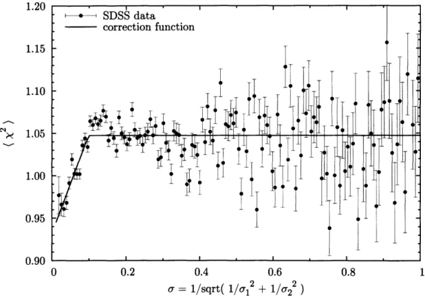
The Lyman-cl forest region of a high-resolution quasar spectrum . . Average X2 as a function of
&
...Example flux PDFs ...
Number of pixels in each redshift bin ...
The shape of the flux PDF as the parameters in the model are varied. Model flux PDF before and after adding noise ...
Signal to noise dependence of best fit values of A and B ... X2 per degree of freedom for the best fit lognormal model ... Best fit A and B for the fourth signal to noise quartile ... The lognormal fit for z 2.2 ...
The lognormal fit for z 2.3 ... The lognormal fit for z - 2.4 ... The lognormal fit for z 2.5 ... The lognormal fit for z - 2.6 ... The lognormal fit for z 2.7 ... The lognormal fit for z 2.8 ... The lognormal fit for z - 3.0 ... The lognormal fit for z - 3.1 ...
The lognormal fit for z 3.2 ... The lognormal fit for z 3.4 ... The lognormal fit for z 3.5 ... The lognormal fit for z 3.7 ... The lognormal fit for z 3.8 ... The lognormal fit for z 4.0 ... The lognormal fit for z - 4.1 ...
The lognormal fit for z 4.3 ...
16 22 23 24 31 32 33 33 36 37 2-1 2-2 2-3 2-4 2-5 2-6 2-7 2-8 2-9 3-1 3-2 3-3 3-4 3-5 3-6 3-7 3-8 3-9 3-10 3-11 3-12 3-13 3-14 3-15 3-16 3-17 3-18 3-19 3-20 3-21 3-22 3-23 3-24 3-25 3-26 40 42 43 44 47 49 50 52 53 54 55 56 57 58 59 60 61 62 63 64 65 66 67 68 69 70 . . . . . . . . . . . . . . . . . . . . . . . . . . . . . . . . . . . . . . . . . . . . . . . . . . . . . . . . . . . . I . . . . . . . I . . . . . . . . . . I . . . I . . . I . . . I . . . . . . I . . . . . . . . . v
3-27 The lognormal fit for z - 4.6 ... 71
3-28 Lognormal model parameter aln for the two limiting values of a. ... 73
3-29 Lognormal model parameter To for the two limiting values of a. ... 74
3-30 r0 and
Teff,compared to other measurements ...
75
B-1 First median composite, medianI. ... 82
B-2 An example spectrum before and after tilt. ... 83
B-3 The difference between medianl and median2 ... 84
List of Tables
2.1 Values of AT(k/H) for the Monte Carlo and analytic calculations ... 38
3.1 Redshift bin characteristics ... 44
3.2 Best fit lognormal parameters and their errors ... 51
Preface
One of the most peculiar features of the observable universe as a whole is how it appears to be so smooth on very large scales and yet be filled with so much structure on smaller scales. The theory of inflation describes a period of rapid expansion in the very early universe and provides a possible explanation for the origin of both of these phenomena. Inflation's
exponential expansion flattened away any initial inhomogeneity, while quantum fluctuations
in the energy density were imprinted onto the density perturbation spectrum emerging from
the inflationary phase and provided the seeds for large scale structure.
While the general predictions of inflationary theory are well-supported by current
cos-mological observations, the details of the theory and an understanding of the transition from the inflationary phase to the one we find the universe in today are not well understood. This thesis approaches these questions from two very different angles in two independentprojects.
First, through detailed calculations of the density perturbation spectrum generated by
a particular model of inflation called supernatural inflation we address the primordial origin of the fluctuations which give rise to observed large scale structure. This project is described in chapters 1 and 2.Second, using observations of the Lyman-a forest in the spectra of quasars we study the subsequent evolution of the distribution of matter in the universe. In particular, we
characterize the redshift dependence of the flux probability distribution function in the
Lyman-a forest in terms of a simple underlying model for the density distribution. This project is described in chapter 3.Chapter 1
The Inflationary Universe
The theory of inflation (Guth 1981; Linde 1982) provides the most complete picture we have of the early universe and receives strong support from recent high-precision measurements of the cosmic microwave background (Spergel et al. 2003). Inflation is characterized by a period of rapid expansion in the very early (10-3 5 sec) universe. This type of expansion is caused by the repulsive gravity effects generated by a scalar field, often called the inflaton field. As the scalar field evolves, the universe is driven into a period of exponential expansion.
The inflationary picture has had remarkable success in explaining several key features of the universe. Inflation drives the universe towards an otherwise improbable flat geom-etry (critical density) and also smoothes out large scale inhomogeneities without the need for acausal physics. Additionally, inflation provides the seeds for large scale structure by
imprinting quantum fluctuations in the spectrum of density perturbations emerging from
the inflationary epoch. All these predictions are borne out in our observations of the cosmic
microwave background.Although the general predictions of inflation are supported by current cosmological ob-servations, the exact mechanisms of the theory are not yet well understood. Many different inflationary models have been introduced, with substantial variation in the precise details, yet no single model has emerged with overwhelming acceptance. A major shortcoming of most inflationary models is known as the fine tuning problem: in order to guarantee suffi-cient inflation as well as the correct magnitude of density perturbations, parameters in the inflaton potential must be fixed at unnaturally small values (generically of order 10-12). While nothing in the theory prevents this from being the case, without an accompanying explanation this seems uncomfortably implausible. Much work has gone into searching for
viable mechanisms to generate this small parameter naturally.
1.1 The Dynamics of Inflation
In conventional inflationary models, inflation ends when the inflaton field rolls down the
hill of its potential energy diagram. The field is subject to quantum fluctuations, however,
which can be treated as small perturbations about the classical solution of the equations of motion. These perturbations imply that the field rolls slightly faster in some places than inothers, resulting in differing amounts of inflation, and ultimately in density perturbations.
1.1.1 Equations of Motion
We work in de Sitter space described by the metric
ds2 =
g,,dx/Idxv
= -dt 2 + e2Htdx2 (1.1)where H is the expansion rate. The infiaton field +(x, t) is described by the Lagrangian density for a single scalar field,
C=
e3Ht [2 e2Ht(VO)2 - v()], (1.2)for some potential V(+). The resulting equations of motion are
q
+ 3H
- e-2Htv2q
=9V
(1.3)
1.1.2 Time Delay Formulation
To study the density perturbations generated by quantum fluctuations in the inflaton field we use the time-delay approach of Guth and Pi (1982, 1985). Begin by writing the field as the sum of a homogeneous (classical) term, o, and a quantum fluctuation, ,
+(x, t) = 0o(t) + 60(x, t).
(1.4)
Substituting this expression into Eq. (1.3) we find that the homogeneous piece satisfies
Qo + 3Ho = a (1.5)
Taking the time derivative of Eq. (1.5) results in the relation
+ 3Hao = qo a2V (1.6)
Meanwhile, the perturbation satisfies
q + 3H6
-e-2HtV
260 =
q-
a2V (1.7)O2V[ 0
The spatial gradient term in the above expression is exponentially damped and at late
enough times will vanish; we will work in this limit. We now see that the time derivative of the homogeneous solution, 4o, and the fluctuation, b, satisfy the same differential equation:d2,
+
d
2Vi (1.8a)dt2 (0) +
(;)
a02 o(.dt
dt2
(60) + 3H dt (60)
=60
2V I (1.8b)The second order equation has two linearly independent solutions, but it can be shown that one of these solutions damps very quickly. Hence at late times both o and 64 are
proportional to the undamped solution, and are therefore proportional to each other. We choose to write the (time-independent, but position-dependent) proportionality factor as a time delay field -r(x), so that
6+(x, t) = -dr(x)
o(t).
(1.9)
In other words, to first order in Tr, the effect of the fluctuations is to produce a position-dependent time delay in the evolution of the homogeneous field:
O(x, t) = o(t - Jr(x)).
(1.10)
Thus, the problem of calculating the spectrum of perturbations in the inflaton field reduces to the (hopefully simpler) problem of calculating the distribution of time delays and making use of the relation in Eq. (1.9). It is important to remember that this is an
asymptotic time delay defined for times sufficiently late that the spatial gradient term in
Eq. (1.7) can be neglected.1.1.3
The Power Spectrum
The relationship between the asymptotic time delay field at the end of inflation and the
resulting density perturbation in the post-inflation universe is discussed by Guth and Pi (1982) and Olson (1976). Here we simply quote the results. The Fourier transform of thefluctuations of the density field are proportional to the Fourier transform of the time delay
field,
6P (k) = 2x/2H &f(k). (1.11)
P
Typically, this expression is evaluated at the (k-dependent) time at which the particular
wavenumber k is crossing the horizon (this is when the fluctuation will have frozen in).We will define the power spectrum as the correlation function of the Fourier transform of the time delay field, Ar(k), where the correlation function is defined as follows. Given a stochastic function f(x), we measure the mean fluctuations of wavenumber k by
1
Af(k)-=
[2
dxeik(f()f(O))].
(1.12)
In Chapter 2 we calculate AT(k) for a model of inflation called supernatural inflation, and the above expression is applied to our particular case. The rest of the details will be
deferred until that discussion.
1.2 Supernatural Inflation
Supernatural inflation is a supersymmetric hybrid inflationary model proposed in 1995
by Randall, Soljacic and Guth (Randall et al. 1996). This model attempts to solve the
fine tuning problem by linking the small numbers in the inflationary potential to existing small parameters in theories of spontaneous supersymmetry breaking. As with other hybrid inflation models (Linde 1994), it becomes possible to separate the physics that determinesFigure 1-1: The inflaton potential V(+) for different values of the field 0b.
the rate of exponential expansion and the physics that determines the magnitude of density
perturbations.
Supernatural inflation accomplishes this through the use of two coupled scalar fields. In this case, the potential energy function of the inflaton field () changes due to the evolution of a second field (), behaving as though it had a time-dependent mass term (see Fig. 1-1). Initially, the inflaton field is at rest at the minimum of its potential energy function V(+).
But the evolution of the second field changes the qualitative shape of this potential energy
function and the inflaton field eventually finds itself perched unstably atop a hill in the potential energy diagram. Quantum fluctuations then cause the inflaton field to roll down this hill. This results in fluctuations in the value of the field, and causes inflation to end at slightly different times in different places. It is in this way that inflation leads to spatial fluctuations in the energy density emerging from the inflationary phase.But in contrast to other models where the dynamics of the scalar field can be treated classically, in the case of supernatural inflation the initial instability of the field is caused by quantum fluctuations. Thus the quantum fluctuations cannot be treated as small pertur-bations about a classical solution, and therefore new methods have to be developed. The problem of determining the variation in the amount of inflation from place to place becomes nonlinear, and the only known analytic estimates are based on untested approximations. Our work has focused on comparing these analytic estimates to numerical simulations of the theory.
Chapter 2
Density perturbations in
Supernatural Inflation
2.1
Overview
In the original supernatural inflation paper (Randall et al. 1996) the authors made an untested approximation so as to be able to solve analytically for the density perturbations; the goal of this chapter is to test the validity of that approach. Traditionally one can solve for the fluctuations about the classical solution of the inflaton field, however for the present model there is no classical solution. The proposed idea is to let the RMS value of the fluctuations play the part of the classical variable. However, it is unclear how to quantify the validity of this approach, and so the intent of this project is to calculate numerically
the perturbation spectrum and to compare with that obtained from this analytic method.
We can only do the numerical calculation in one dimension. However, if the ansatz holds in one dimension, so that the perturbation spectrum calculated analytically is consistent with the one computed numerically in one dimension, we have a substantial reason to believe the results it would give in three dimensions are also right. Throughout this Chapter we specialize all formulae to the particular case of one-dimension (nd = 1) unless explicitlystated otherwise.
2.2 Numerical Integration of the Mode Functions
We assume a fixed background de Sitter space, with a scale factor given by
R(t) = eHt .
(2.1)
The scalar field 0 is then described by the Lagrangian density
1 2
L eHt2 [ 2 -e-2Ht(Vq)2 2m~(t)k2 (2.2) where we are allowing a time-dependent mass term. The mass is actually controlled by the
4'
field, which in our approximation will also be described as a free scalar field, but thistime one with a fixed mass:
t=
eHt
[2
_-
e-2Ht(vO)2
_
m
/2].
(2.3)
The expressions for the Lagrangian densities are valid up to an additive constant, which is defined to have whatever value is needed to sustain a Hubble constant H. We will treat H as a constant.
The equations of motion for 4 are given by
a
(eHte)
_ a
(eHte 2Htaio) =-eHtm2(t)o (2.4b)or finally
; + ndHq - e-
2HtV
2, = -m (t).
(2.5)
Similarly,
+ ndH2 - e-2HtV2 = -m2Ib. m
(2.6)
We approximate the 0 field as homogeneous and slow-rolling, so that the k term is negligible, and therefore
'(t)
= const x e-(m/H)t
(2.7)
The value of the constant is arbitrary, since it merely fixes the origin of time. We choose
the constant so that
4'
=
2Ck
at t = 0, where %c
is the value of b such that m2(t) = 0. Thus,
l(t)
= Oce-(m /ndH)t . (2.8)We switch to definitions in which H is scaled out,
N Ht,
(2.9)
I+
_ -
m,/H,
(2.10)
and so
+'(t)
= ce-
VN
(2.11)
For notational convenience further define the quantity
1 1 (2.12)
We
will
erm proporional o
take
o have
a
H2where for the numerical
simula-We will take m (t)to have a term proportional to 0b
r,
where for the numericaltions we will take r = 4. We can then write
m+(t)
=
-m2 [1-(t
))]
(2.13)
=m21
( r=-m
[11- e-(rlN1] .
(2.14)
Scaling again by H, we define
P mo/H . (2.15)
2.2.1
Obtaining the Equations Governing Mode Function Evolution
We quantize the field following the formalism of Guth and Pi (1985). The setup of the lattice will be described in detail in section 2.3. As described more fully in that section,
we expand the field +(x, t) in terms of quantum creation and annihilation operators, and
the mode functions u(k, t). Eq. (2.40) defines the relation between the field +(x, t), whose behavior is governed by its equation of motion Eq. (2.5), and the mode function u(k, t), which we will numerically integrate.The equation of motion for the mode function u(k, t) is
ii +
i
+ e
2N
k 2=u
-
[1-eN
] u
(2.16)
where the dimensionless wavenumber is
k- [k[ (2.17)
We define the functions R(k, t) and 0(r, t) such that
u(k, t)
R(k, t)ei(k
' t)(2.18)
2kH
which allows us to separate the real and imaginary parts of the differential equation,
R-R
2
+
R +
-NkR
=
[1-e- aN] R,
(2.19a)
2iRt + iRO + iRO = 0. (2.19b)
The second equation can be integrated, and matched with the early time solution, to give an expression for 9
ke-N
t -- R'ke (2.20)
which we substitute back into Eq. (2.19a) to give a single, second order differential equation for R:
e-2Nk
e-2Nk22
-2a2
N
-
3 + + e-
2Nk
2R =
[1
-e-N]
R.
(2.21)
method we split this into two, coupled, first order equations. Let R S, so that
S - R -R+R
[4 (1-
e-PN)
-k2e2N]+
R
(2.22)
The equations to be solved are thus:dR
=d
= R(2.23a)
dN
dO ke-N d-= +-
- +(2.23b)
dN
R
2 2 -2NdN=
_ -+ R
[I
(1-
e- N)
k2e-2N] +
(2
Note that these equations are cast entirely in terms of dimensionless quantities. They completely specify the mode functions, as a function of time, once two initial conditions are specified; this is the topic of the next section.
2.2.2 The Initial Conditions
At early times the term proportional to k2 in Eq. (2.16) dominates over the term
propor-tional to p2. Dropping the latter results in a differential equation which has an analytic
solution, so we use this asymptotic early-time solution as the initial condition for our nu-merical solution of the full equation.The equation describing the early-time behavior is solved by a Bessel function. We evaluate the Bessel function at asymptotically early times and find that the initial condition for R is that
R(N
-oo) = 1.
(2.24)
However, to begin integrating early enough that this initial condition is accurate would require starting so early that the equation is difficult (and in some regimes impossible) to numerically integrate. The function R behaves like a simple harmonic oscillator with a
time dependent spring constant -
the spring gets stiffer and stiffer in the past, so that
tiny perturbations about the minimum result in large oscillations. This in turn makes it
even more important to start with the field precisely at the minimum of its potential, so
the earlier you begin integrating the more accurate the initial condition must be.We solve this problem by including higher order terms in the Taylor expansion of the early-time solution so that the initial condition is sufficiently accurate even at "late" times when it is straightforward to integrate Eq. (2.23). Let the solution at early-times be:
R(N) = 1 + 6R(N)
(2.25)
and substitute this into Eq. (2.21). By a clever grouping of terms, one can generate succes-sively higher order corrections to the initial condition Eq. (2.24). The expansion we work with is:
JR(N)
= R2 2+ R24 + SR26+ R4 4 + R4 6 + SR6 6. (2.26)respectively, these terms are found to be: e2N
SR
22 =4
__1
N]
(2.27a)
5R
24= 1-4 [e-N
-(2
)(3
-
2
)
-
6]
(2.27b)
6R26 =-2 -e
[e-~N(2
-_2)(3
_
2)(4-
2)(5-
)- 120]
(2.27c)
SR
44=50320
[1
-e-I2
(2.27d)
SR
4=
6e-
[2N(
2 -2)(37 -14i) -
ei
(148-65 + 9) + 74
(2.27e) 6 e6NR66
= 15128k6
[1-e
N](2.27f)
Note that this expansion is only valid in the region where JR < 1. However, truncating the
series after only six terms would become a bad approximation long before this inequality is
violated so in practice we do not need to worry about approaching this regime.A similar procedure can be applied in the case of . From the Bessel function
describ-ing the asymptotic early-time solution we see that the initial condition for the angular
component of the mode function isO(N -* -oo) = ke
- N-
7r/2.
(2.28)
Since the dynamics will not be affected by an overall phase redefinition, for simplicity we
will drop the term 7r/2. As with R we expand the early-time solution as the asymptotic
solution plus a correction0(N)
=eN (k
+
60(N))
(2.29a)
' e- N (k + 6022 + 6024 + 6044 + 6026+ 3046 + S066)- (2.29b)
At early times the differential equation for 0 can be expanded as
*= ke
- N9=- RR 2 (2.30a)
_ ke-N(-1 + 25R - 3R
2+ 45R
3)
(2.30b)
where in the last line we move the time dependence to the numerator by using the expansion
R
- 2= (1 + R)
- 2= 1 - 2R + 35R
2- 4SR
3+ 0(6R
4).
(2.31)
This can be integrated analytically after inserting the expansion for R in Eq. (2.27). Using
analogous notation to the previous case the leading terms are:
10" 1010 100 10-10 l ,-20 S f rn Size of 5R correction, k/H = 256 IU -10 1020 1010 100 10-10 i n-20 5 Ht JU -10 5 Ht 10v 10-10 10-20 10-30 n,-40 IU -10 100 10o-o10 10- 20 10-30 10-40 -5 0
Ht
Size of 50 correction, k/H = 25624
5044-6066 -10 -5 Ht 0 5 5Figure 2-1: Size of the leading six terms in the expansion of JR and J9 for a representative
small wavenumber k/H = 0.004 and large wavenumber k/H = 256.
(2.32b) (2.32c) 6024 =-
8k3
[2
- e(2-aN 4e4 6e- N 3e2 N 3044 =
24k
3[1
3-f
+
3
2
26
=
N- [e -,
N(
2-
i,2)(3-
_i)(4-
t)-
24]
6026 -- 5 le32k 4 6N[
046=-
-
56-160k5 10e- N (56 - 25 , + 3A,) 5e- 2N (2 - )(28 5- A2 5 - 2pf (2.32d)- 112)
(2.32e) 5066 = 80k5 [ 15e-N V 5 - 2 15e-2N P+5 - 22
5e-3NP45 - 32 .
(2.32f)The first six terms in the expansions for AR and
39
are plotted in Fig. 2-1.The procedure is to determine R and 0 by these formulae at early times when the expansions are sufficiently accurate, and then transition to numerical integration when the expansions begin to fail. The next section describes how to determine this transition time.
- -9 Size of JRcorrection, k1H = 1/256
0
-5
-10
-15
sTime (err.
.
in expansion < 108
!
sTime (error in expansion < 10-8 )0.001 0.01 0.1 1 10 100 1000
k/H
Figure 2-2: The transition time (sTime ) after which the trajectories are computed by
integration rather than by evaluating the initial condition expansion. Determined by finding
the time the term 6026 or SR26 = 10-8. The "earliest possible integration time" is when the integrator first fails
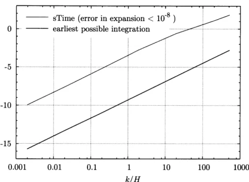
2.2.3 When to Begin the Integration?
The corrections R and 60 only provide a good approximation to the true solution of the mode function equation so long as the size of the correction is small, or more precisely, so long as the first omitted term in the expansion is negligible.
We determine the time when it necessary to transition to numerical integration by finding the time when the first neglected term reaches some specified value. In practice, we find that in the regime we are interested in the smallest of the six terms are R26 and 6026 (see Fig. 2-1; note that for the left-hand figures which show the low wavenumber, this
transition time is well before the crossover around Ht
.-5 when R
26ceases to be the
smallest of the six terms). The size of the omitted term in each expansion is thus bounded by this value and so we locate the time when max[6R26, 6026] equals a predefined constant
which we have chosen to be 10-8. Fig. 2-2 shows, as a function of wavenumber, this time (which we call "sTime") when it is necessary to transition to integration. Also shown in the figure is the earliest possible time the numerical integrator will function. Anytime between the two curves would be fine to use as the starting time, for computational efficiency we of course go with the latest acceptable time.
We aim for a numerical accuracy of 10-6 in the final determination of the power spec-trum, so to be conservative we aim for an accuracy of 10-8 in the mode function integrations. For the function R this means we require the fractional error between the true solution and the numerically obtained solution to be AR/R < 10- 8. In contrast, for the phase 0 it is
the absolute error AO < 10-8 that matters since it is the number modulo 27r which affects
the dynamics.
Fig. 2-3 demonstrates that finding the trajectory by evaluating the early-time
expan-~kI
i1~O LrJ'J"0i 0.1J I..LO jiLCbtJ1V
... . I . . .. . ... .. . ... ... ... . . i. . . i . . . . I . . · · · __ _ __ _ __ _ _ - r~n
~
\ ;---~rr ..~r
---- --- ---:--- --- ---... -- ... J ... --- _---... --- --- ------10- 9 10 -10
I
10-11 10-12 1n-13 1U -10 -5 0 5 Ht .^n-7 1 ' 10-8 10- 9 10-10 < 10 10-11 10- 1 2 1n-13 -10 -5 0 5 HtFigure 2-3: Errors in trajectories resulting from evaluating earlytime expansion for times
earlier than sTime rather than integrating directly. These curves resulted from setting the
error tolerance (size of first neglected term) at 10-8. The top plot shows the fractional error in R for a range of relevant modes, the bottom shows the absolute error in 0 for the same modes.
sion up until the the time when max[6R26, 6026] = 10-8, then numerically integrating the
remainder of the trajectory, is accurate to about one part in 108 compared to integrating the entire trajectory. In fact the 6026 constraint is generally the more stringent of the two and so at sTime , 6R26 is still smaller than 10-8 leading to an even smaller error in R.
2.3 Formalism of Constructing the Inflaton Field
We work on a one-dimensional lattice of fixed coordinate length b with Q independent points and periodic boundary conditions. This means that the position variables are restricted to
the locations
b
xi = (2.33)
Q
where the integer i which indexes the position can take on any of the Q values from 0 to
(Q - 1). Note that because of the boundary conditions, xo = 0 is identified with XQ = b.
In our calculation, Q will always be an even power of 2.
The corresponding allowed values for the wavenumber k are:
kn
= -n (2.34)where the integer n can take on the Q values from - to (- 1). Again the periodic boundary condition identifies the first and last mode, k_Q/2 = kQ/2, and we keep the former.
When it is necessary to convert between sums and integrals we use the relations
Jdx
f
(x) =
x f(x)=
()
f(x)
(2.35)
dk f (k) = aZ k f(k) =
(
b
f
(k).
(2.36)
Our Fourier transform convention is
f
(x) = dkeik f(k)
=
(
)
eik
f
(k)
(2.37)
f(k) = 2-Jdxe-ikz f(x) =
( )
()
ei
f(x).
(2.38)
To convert to dimensionless quantities for the numerical calculation we measure the box size in Hubble lengths,b bH, (2.39)
when appropriate. Note that b is the coordinate (comoving) length of the box and so the physical size is equal to bphys(t) = beHt.
2.3.1
Setup
For a complex scalar field +(x, t) in one dimension
1
O(x,
t)
=
j
(+
)
21: [c(k) eikxu(k, t) + dt(k)
e-ikxu*
(k,t)1
.(2.40)
Here the summation over k is an abbreviation for summing from n = -Q/2 to (Q- 2)/2,
the u(k, t) are the mode functions computed in the previous section, and ct(k)/c(k) and
dt (k)/d(k) are independent complex quantum mechanical creation/annihilation operators1.
Note that the field +(x, t) is dimensionless since u and V~ have the same dimensions. Since the sum is over both positive and negative values of k we are free to replace
-k - k in the second term of the summation giving
(x, t)
=b-
Ee
i kx[c(k)
u(k,
t) + dt(-k) u* (-k, t)].
(2.41)
k
Now calculate the Fourier transform,
1 b
[(k,
t)=
27 Q Eeikx(,
t)
(2.42a)
(2.42a)
x
1 b2
e-i eik' [c(k')u(k',t) + dt(-k')u*(-k', t)]
(2.42b)
=
1Q
6k,k'[(k')u(k',t) + dt(-k')u*(-k', t)]
(2.42c)
rb2
[c(k)u(k,t)+ dt(-k)u*(-k,t)].
(2.42d)
Notice the following useful relation2 obtained by equating the righthand sides of Eq. (2.42a) and Eq. (2.42d)
E:
e-ik(x,t)
=
[c(k)u(k, t) +
dt-k)u* (-k,
t)]
(2.43)
The field (k, t) has the dimensions of length. When we need it, the dimensionless version of this field will be:c(k, t) - HO(k, t).
(2.44)
2.3.2 Operator Normalization
We will now verify that as defined in Eq. (2.41) the quantum operators c and d are normal-ized correctly. We begin by finding an expression for c(k). First, take the time derivative of Eq. (2.43)
-
Ze-ik
(x,
t) = [c(k)
i(k, t) +dt(-k) i(-k, t)] .
(2.45)
Next multiply Eq. (2.43) by i*(-k, t) and Eq. (2.45) by u*(-k, t), and then subtract
Ee-ikx
[i*(-k, t)(x, t)-
u*(-k,t)x,
t)]
c(k) [u(k,
t)
i*
(-k, t)
-i(k, t) u*(-k, t)] .
(2.46)
It turns out that the quantity in the brackets on the right hand side is equal to the
2The following relations are also useful: E. e(k- k '
Wronskian which we can calculate directly in this case. Following the method in Guth and Pi (1985), we consider the quantity
W(k, t) _ u(k, t)
(-k,,
u
*
t)
(2.47)
at
at
Then
W(k, t)
2u*(-k, t)
_a2u(k,t)
=u(k,
t)
*(-,t)
(2.48)at
at2 at2since the terms involving products of first derivatives cancel. Using Eq. (2.16) to replace the second derivatives, one finds
(kt) =
t
HW(k, t)
(2.49)
at
which is easily solved to give
W(k, t)
= f(k)e
-Ht
(2.50)
where f(k) is an arbitrary function of k.
Since f(k) is independent of time, we can evaluate it for our choice of functions u(k, t) by computing its value at asymptotically early times, when u(k, t) is given by [I'm still missing the early-time DEQ equations]. Then using the Hankel function identity
H d H(2
dz
Z)Z_(2)(z
-
z)
dH(1)
=
--
4i(2.51)(2.51)
one finds for k 0 that
W = ie
- Ht.
(2.52)
This is the one-dimensional analogue to the formula derived by Guth and Pi (1985) for the
case
nd= 3, where they find W = ie
- 3 Ht
We can now return to Eq. (2.46) and insert this expression for the bracketed term on
the right hand side:
I
E
e-ikx[i*(-k,
t)o(x, t)- u*(-k, t)x,t))]
=
c(k) [ie-Ht].
(2.53)
Thus,
c(k)
=-ieHt 0(
)
x
e-ikx[*(-k, t)q(x, t)
-u*(-k, t)(x, t)] .
(2.54)
We can apply a similar procedure to solve for the second operator,or conjugating,
d(k)
=-ieHt(b)
eikx[t*(-k,
t) *(x, t) u*(-k, t)4*(x, t)
(2.56)
Note that c(k) and d(k) differ only in that -, b*.
We now verify that the normalization was chosen correctly by computing the various commutators. The Lagrangian density for the field +(x, t) is:
C
= e
H[-
e-2Ht(VO*)(V)-mg(t)l *dl]
(2.57)
Note that the familiar factors of Note that the familiar factors of 1 are missing, but that is simply because this is a complex1 are mis~;rrrr ~rr~ +~o+ ;n ~;m~l~r ha~arr~n ~
field. It is equivalent to writing L£(q)
=
C(c0l)+
f£(02)where
4 = -2(cl + i
2).
Replacing
the usual integral with a sum, we obtain the Lagrangian
L = e -
E
e-(2.58)
L
= e~t(Q)
[~-
e-2Ht(V'*)(V+))-m+(t)[b*+|]*
(2.58)
The canonical momentum for a complex field is given byr(z
_a.L
= et (x). (2.59)The canonical commutator,
[+(x), 7r(x')] = ix,x,, (2.60)
implies that
[+(x),
*(x)] =[*(x),
4(x')]
=ie
H t(Q)
x,,
(2.61)
For the complex field case we will need another variation of this commutator. Expanding out the field in terms of two independent real fields as before, q = (l + i 2), we find
[4(x),
+(x')] = ¢,, - ¢,¢ (2.62a)= ((01
+ if
2
)(
1
-
+
if
2
) - (1 + i
2
)(Ol
+ i
2
))
(2.62b)
=
([~i,
il]
-
[P2,b2]
+ i[ol, 02] + i[ 2,li]
)(2.62c)
([1, 1- [2, 02] ) (2.62d)
= 0 (2.62e)
where we have used the fact that the crossterm commutators vanish since the fields are independent.
op-erators. To simplify the following expressions we adopt the notation u-k - u(-k, t).
[c(k),ct(k')]
=
e2Ht
b
eike-ik{(
-
k'x
- Ukx)(Uk',_kx)
x,x
(itUkq'x
-
kxU-'u)(kxUkqx)}
(2.63a)
2Ht
b
iktxte-ikx ~* u*=e2Ht
6
ek eikx (-Uk'* k[x,q*,]
+ ilkU* k[4) 4x4X])
(2.63b)
x,x,
= e e2Ht
b
- eik eeikx
e (ieHt ie - J (Uk uXlcruX/e f k+
~cl~lu-
kU k)(2.63c)
x,x
Qx
= ieHt
k k'Q(-ie-Ht)
(2.63e)
Q
= 6k,k'- (2.63f)
In Eq. (2.63d) we again used the Wronskian3
. Next compute the mixed term:
[c(k),
dt(k')]
=e2Ht
b
eike-ikx
{
(u x -Ukx)(uk''u-k
)x,xi
(ikl'Ox'
-
UkAZ)(iU
_klx
-
U*kx)}
(2.64a)
2Ht b E Z'x' -'k
e2Ht 6 eik''eikx (- Uk-k/ kk[x x
~x']
+ U1k'U k[Ox', Qx)(2.64b)
x ,x
=O (2.64c)
by Eq. (2.62). Applying a similar procedure to the remaining combinations, one finds that the other combinations also produce the expected result and we see that the normalization is indeed correct. In summary,
[c(k),
ct(k
') ] = [d(k), dt(k')]= k,k
(2.65)[c(k), d(k') = [c(k), dt(k')] = [ct(k), d(k')] = [ct(k), dt(k')] = 0.
(2.66)
2.4 The Monte Carlo Approach
In this section we calculate the time delay directly by following the individual mode trajec-tories.
3
2.4.1
Calculating (k,t) and O(x,t)
Having computed the value of each mode function uk at a given time we construct 0(k, t) as follows.
The mode functions (Eq. (2.18)) are:
(k, t) - R(k, t) ei(k,t) (2.67)
Note that the mode function only depends on the magnitude of k, so it is fine to replace
u(-k, t) - u(k, t) and we have from Eq. (2.42)
l
(k, t) = 2 (c(k)u(k, t) + dt(-k)u*(k, t))
(2.68)
The quantum operators are formed from Gaussian random numbers (ai),
c = al + ia
2(2.69)
dt = a3 - ia4. (2.70)
These random numbers are independent of time; a set of four ai's are drawn once for each k. They are chosen from a Gaussian distribution with width a = 0.5, since the normalization
of c gives: 1 =
(OIc
tcIO)
((al-ia
2)(al
+ia
2))= (a
2+a22) = 2(a
2), resulting in (a
2) =
After multiplying out all of the products and collecting real and imaginary terms, we find:m [4(k.t)]
=2
2
R [(a2-
a4) cos+ (al-aa
3) sin 9]
(2.71a)
e [O(k, t)] =
2
R a + a3) cos 0- (a2 + a4)sin0 (2.71b)The dimensionless counterparts,
bH ,
k -kH,= uv-H, and N = Ht give
am
[(k, N)] = 2
L
R [(a
2-
a
4)cos
0+ (al- a3)sin ]
(2.72a)
Re [(k), N] =2
AR
[(al + a
3)cos 0- (a
2+ a4)sin0 ].
(2.72b)
To compute
10(x,
t)l - (Re [O(x, t)]2 + Qm [(x, t)]2) 2 we use a standard fast Fourier transform routine from Numerical Recipes.2.4.2
Advancing (x, t) in Time
The field O(x, t) can be computed straightforwardly by computing the values of the mode functions uk at at a series of different times, then computing the FFT of the complex components of q(k, t). Each new time step would require an additional FFT and knowledge of 4b(x, t) at some previous time provides no help in finding the amplitude of the field at some new time owing to the non-linear dependence on k in the Fourier transform.
-0 IU-- -2 > 10--t 10- 6 CeS-o- 10
d
10
- 8 ln-1 0 0 5 10 15 20Ht
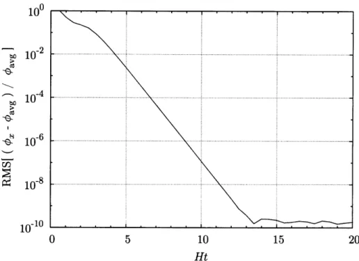
Figure 2-4: The RMS of the distribution of fractional errors between individual +(x, t)
trajectories and the average. We see that to high accuracy (> 10-8) they have reached
the common trajectory by a time of N = 12. Note that the flattening out after N > 14 is simply due to the fact that the trajectories were only saved to ten digits of precision.
However the situation in practice is significantly better. The k-dependence in the
equa-tion of moequa-tion (Eq. (2.16)) enters via a term proporequa-tional to
e-2Ht.This means that at late
enough times the k-dependence drops out and from that point forward the modes evolve identically. Of course the amplitude of each mode function entering this regime will be a complicated function of the full k-dependent dynamics earlier on in the trajectory, but it means that at late enough times the subsequent behavior is quite simple (in fact, nearly exponential). Since the k-dependence drops out of u, it will also drop out of 0(x, t).To be specific, for some time N >
Nlate
the field at each point x evolves viaO(x, N)
(X
aN) = f (N), independent of x.
(2.73)
O(x, Niate)
The goal is to find both the function f(N) and the time Nlate after which f(N) accurately
advances +(x, Nlate) forward in time. Once we know that, we simply need integrate each mode up to Nlate, perform a single FFT, and then employ f(N) to determine +(x, N) atany subsequent time.
To determine this time when the trajectories reach the stage of k-independent evolution,
compare various individual +(x, t) trajectories to the average trajectory. The spread of
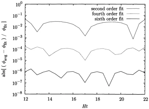
values relative to this average field avg(N) = E., O(x, N)/Q decreases at time increases, and by a time of N = 12 the deviations are well within our tolerated error. Fig. 2-4 shows the evolution of this spread.We determine the function f(N) by fitting the exponential of a high order polynomial
to the average trajectory avg(N). To achieve an accuracy of 10- 6 it turns out we need a100 10- 1 10- 2 10- 3 10- 4 bO -_S cd 10- 5 10- 6 10- 7 1n-8 IV 12 14 16
Ht
Figure 2-5: This is for fit performed over the range
of relative error is < 10-6 in this range. Note that
and so it is not meant to be extended to later times.
18 20 22
N = 12 - 22. Average absolute value
outside of this range the fit diverges
sixth order polynomial,
f
(N)
= 1 0(co+clN+c2N2+c3N3+c4N4+c5N5+c6N6) (2.74) Fig. 2-5 shows the accuracy attained using various order polynomials, and Fig. 2-6 showsthe average trajectory and the resulting best fit.
2.4.3 Finding the Time Delay Field
As a result of the previous section, we can easily determine +(x, t) at any late time. The next step is to compare the amplitude to the value of some specified constant bend which
defines the "end" of inflation. The position-dependent time r(x) when [0(x, rT) = Oend is
the desired time delay field.
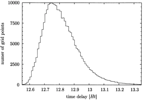
What we actually need to do is invert the function in Eq. (2.74) so that given a value of +(x, Nlate) it will return the time you would need to advance to in order for the amplitude to be equal to bend. This is done using a simple Newton-Raphson root finding routine. Fig. 2-7 shows an example distribution of time delays resulting from this procedure.
2.4.4 The Power Spectrum in the Monte Carlo Case
Functionally,
FFT to r(k).
and then caneach "run" will give a single instance of the time delay field r(x) which we We need many instances of r(k) (each using a new set of random numbers) find, as a function of k, the RMS value.
1030 1025 1020 1015 10lo 105 100 12 14 16 18 20 22
N= H t
Figure 2-6: Average trajectory and the resulting best fit.
10000 7500 5000 2500 0 12.6 12.7 12.8 12.9 13 13.1 13.2 13.3 time delay [HtJ
Figure 2-7: An example time delay distribution from a single run with a lattice size of
Q = 218 points and end = 1018.
The power spectrum derived using Monte Carlo approach is then computed by
ATmc(k) = [2brr
(l'r(k)
(IT(k)12)1 12] 2 (2.75) (NI X -,sX M o © o E)The derivation of this formula is given in Appendix A.
2.5 The Analytic Approach
Our goal is to compare the power spectrum obtained using the method described in the
previous section with the power spectrum obtained using the analytic method described
below.2.5.1
Calculating
rmsIn the analytic approach we let the RMS value of the classical wave packet play the role of
the homogeneous solution Oo(t) about which to study perturbations,
qrms(t)
vlwo)-(2.76)
-This notation is shorthand for (l *(x) k(x)10) where 10) is the vacuum state. We can use Eq. (2.41) to expand this expression:
(*)
=
b-1l
e-ik eik'x (Ock U +
d-k U-k) (Ck' uk'+
Udk,
k)).
(2.77)
k kt
The operators c and d are annihilation operators. Terms which contain an annihilation
operator acting on the vacuum will vanish, d0
)= 0, and likewise (Oldt
( d0) )t = 0.
The only term in the expansion of the product that does not involve annihilating the
vacuum is the term containing d dt and we can use the commutator in Eq. (2.65) to reorderthe operators:
(01(
u +
+
(
dkuk)
u)
c
+
dt
ku,)
0o
)
= Uk
u,
(01dk
dt,
o)
(2.78a)
=k U, (1o [dk, dt k] + dt k, dk
) (2.78b)
= Uk Ul
(o
l-k,-k'
o)
(2.78c)
=
luki
26k,k'.(2.78d)
Combining the two previous equations we find
Orms(t)
= b-Z
u(kt)l2)
= E2j
2k
)(2.79)
Next we calculate the time derivative,
rms(t) drms
(2.80a)
dt
/ 1 1
1
R(k,
t)2
(
R(k, t)R(k,t)
(2.80c)
These sums can be carried out numerically from the same mode function integrations used in the Monte Carlo method.
2.5.2
Calculating nAO(k,
t)
The final step is to calculate the the correlation in the field
q$(k,
t). The details are givenin Appendix A, and the result is
A4b(k)=
[b
*(k)(k))
-2v/-
(2.81)
2.5.3
The Power Spectrum in the Analytic Case
Putting these results together we obtain
ATana(k)
-AtO(k,
t)
(2.82a)
fqrms (t) t=tend(k)
= b R(R(k, tana)R(ktana)
,- 2 R(k, tana) R k ,)
i
Z
Ik
)
(2.82b)-r JIkl Ikl
The time that the right hand side should be evaluated at, tana, not entirely obvious. We use the mean time that inflation was found to "end" in the Monte Carlo simulation (which of course depends on bend). In practice the range of ending times is a narrow enough distribution that there is only a small change in the resulting power spectrum over this
range of time.
2.6 Comparing the Results of the Monte Carlo and Analytic
Methods
Fig. 2-8 shows the result of computing the power spectrum by each method. Numerical values are also listed in Table 2.1. The results agree qualitatively. The striking thing about
the particular way the two curves disagree is that applying a multiplicative offset to both
axes happens to align the curves to a remarkable degree. Fig. 2-9 shows the result ofapplying the transformation
kshift =2.19 k, and
ATshift =0.625 Ar, to the analytic curve.
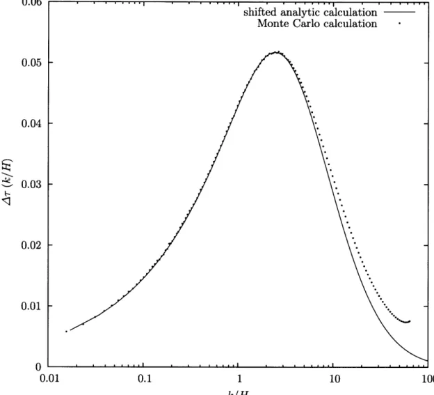
We are actively investigating the connection between the parameters in the theory and the observed offset in hopes of understanding the physical root of the shift.U.1 0.08 0.06 0.04 0.02 n v 0.01 0.1 1 10 100
k/H
Figure 2-8: The final computed power spectra. These curves result from a lattice with
Q = 218 points and the numerical simulation was run 5000 times and averaged.
rN nrP U.UU 0.05 0.04 - 0.03 0.02 0.01 n 0.01 0.1 1 10 100
k/H
Figure 2-9: The result of shifting the analytic curve from Fig. 2-8 in log-space until the
peaks line up and scaling the amplitude so the peak heights match: khift = 2.19 k, and
k/H
0.0156 0.0234 0.0312 0.0428 0.0585 0.0741 0.0935 0.125 0.167 0.222 0.292 0.382 0.502 0.666 0.880 1.16 1.52 2.01 2.66 3.51 4.63 6.10 8.05 10.6 14.0 18.5 24.4 32.2 42.5 56.1 MC 0.0059 0.0070 0.0083 0.0096 0.0112 0.0126 0.0143 0.0165 0.0187 0.0216 0.0250 0.0282 0.0324 0.0364 0.0409 0.0452 0.0488 0.0512 0.0517 0.0499 0.0466 0.0416 0.0358 0.0298 0.0240 0.0189 0.0146 0.0111 0.0087 0.0075Table 2.1: Values of Ar(k/H) for the Monte values correspond to the results plotted in Fig.
2-analytic
0.0136 0.0167 0.0192 0.0225 0.0254 0.0288 0.0332 0.0382 0.0441 0.0500 0.0568 0.0640 0.0709 0.0771 0.0813 0.0826 0.0804 0.0747 0.0663 0.0561 0.0454 0.0351 0.0260 0.0185 0.0126 0.0083 0.0052 0.0032 0.0019 0.0011Carlo and analytic calculations. These
-Chapter 3
Evolution of Structure in the
Lyman-c Forest
Historically, galaxy surveys have provided one of the only observational windows into the evolution of large scale structure. Modern astronomical techniques have now broadened this window significantly, and observations of the Lyman-a forest are probing structure in the universe at an earlier epoch and over a range of scales never before accessible. This provides a crucial link between the complex structure of galaxy clusters today and the early, smooth universe predicted by inflation and measured in the cosmic microwave background. The Lyman-a forest is poised to play a central roll in understanding how our universe
underwent this transition.
3.1 The Lyman-a forest in the Spectra of Quasars
The Lyman-a forest arises from the scattering of UV photons from a background QSO by neutral hydrogen along our line of sight. Photons with energy equal to the Lyman-a trLyman-ansition (1215.67A) Lyman-are reLyman-adily Lyman-absorbed by the intervening neutrLyman-al hydrogen, but the
absorption features are spread out in the observed spectra because the photons redshift
as they travel through the expanding universe. Consequently, each line of sight presents a one-dimensional map of density fluctuations in the universe (Rauch 1998). An example spectrum is shown in Fig. 3-1.The observed flux in the Lyman-a forest region of a QSO spectrum is dependent both on the initial QSO emission (the underlying QSO continuum) and on the subsequent absorp-tion of some fracabsorp-tion of these photons by intervening matter. If one knew the underlying