HAL Id: hal-00317506
https://hal.archives-ouvertes.fr/hal-00317506
Submitted on 31 Jan 2005
HAL is a multi-disciplinary open access
archive for the deposit and dissemination of
sci-entific research documents, whether they are
pub-lished or not. The documents may come from
teaching and research institutions in France or
abroad, or from public or private research centers.
L’archive ouverte pluridisciplinaire HAL, est
destinée au dépôt et à la diffusion de documents
scientifiques de niveau recherche, publiés ou non,
émanant des établissements d’enseignement et de
recherche français ou étrangers, des laboratoires
publics ou privés.
Polar F-layer model-observation comparisons: a neutral
wind surprise
J. J. Sojka, M. David, R. W. Schunk, A. P. van Eyken
To cite this version:
J. J. Sojka, M. David, R. W. Schunk, A. P. van Eyken. Polar F-layer model-observation comparisons:
a neutral wind surprise. Annales Geophysicae, European Geosciences Union, 2005, 23 (1), pp.191-199.
�hal-00317506�
SRef-ID: 1432-0576/ag/2005-23-191 © European Geosciences Union 2005
Annales
Geophysicae
Polar F-layer model-observation comparisons: a neutral wind
surprise
J. J. Sojka1, M. David1, R. W. Schunk1, and A. P. van Eyken2
1Center for Atmospheric and Space Sciences, Utah State University, Logan, Utah 84322-4405, USA 2EISCAT Scientific Association, Box 164, SE-981 23 Kiruna, Sweden
Received: 20 February 2004 – Revised: 22 December 2004 – Accepted: 3 January 2005 – Published: 31 January 2005
Part of Special Issue “Eleventh International EISCAT Workshop”
Abstract. The existence of a month-long continuous database of incoherent scatter radar observations of the iono-sphere from the EISCAT Savlbard Radar (ESR) at Longyear-byen, Norway, provides an unprecedented opportunity for model/data comparisons. Physics-based ionospheric mod-els, such as the Utah State University Time Dependent Iono-spheric Model (TDIM), are usually only compared with ob-servations over restricted one or two day events or against climatological averages. In this study, using the ESR obser-vations, the daily weather, day-to-day variability, and month-long climatology can be simultaneously addressed to iden-tify modeling shortcomings and successes. Since for this study the TDIM is driven by climatological representations of the magnetospheric convection, auroral oval, neutral at-mosphere, and neutral winds, whose inputs are solar and ge-omagnetic indices, it is not surprising that the daily weather cannot be reproduced. What is unexpected is that the hori-zontal neutral wind has come to the forefront as a decisive model input parameter in matching the diurnal morphology of density structuring seen in the observations.
Key words. Ionosphere (Ionosphere-atmosphere interac-tions; Modeling and forecasting; Polar ionosphere)
1 Introduction
The high-latitude ionosphere is known to be controlled by both solar EUV and magnetospheric precipitation and con-vection drivers, as well as the thermospheric responses to these drivers. Since 1993, extensive high-latitude observa-tion and modeling campaigns have been conducted through the NSF CEDAR High-Latitude Plasma Structures (HLPS) working group, in collaboration with the international STEP Global Aspects of Plasma Structures (GAPS) working group. Progress in this research area has been published as special issues of Radio Science in 1994, 1996 and 1998. During this
Correspondence to: J. J. Sojka
HLPS/GAPS decade of research the role of the neutral atmo-sphere and neutral wind has been generally assumed to be small. Many modeling studies have adopted the MSIS model (Hedin, 1987) for the neutral atmosphere and the HWM model (Hedin et al., 1991) for the neutral wind, while mea-surements of the neutral parameters were generally not used in these studies. In the past few years researchers have begun to reconsider the role of the neutral atmosphere, especially its high-latitude representation by climatology models.
As an example of this situation, in the early phase of the present study when it was found that the model runs were not matching the observations, initially no suspicion fell on the neutral wind input; rather the magnetospheric convection and auroral precipitation inputs were the focus of investigation. Later it was found that a change in the neutral wind input could result in a surprising change in the TDIM model cli-matology, bringing it closer to agreement with the observa-tions; this is the specific topic of this paper. The neutral wind at high-latitudes has historically been viewed as primarily a horizontal wind blowing from the sunlit dayside over the po-lar region towards midnight. A simple representation of such a wind was developed by Murphy et al. (1976). Such a wind has been viewed as not effective in terms of the ionosphere at high-latitudes, because the magnetic field lines are nearly vertical, and therefore the horizontal wind will induce only a negligible vertical drift. A second process is that ion-neutral frictional interactions, Joule heating, occurs in the reference frame of the neutral gas, which in general at high-latitudes is significantly less than the convection speed and hence is in general a second order correction term.
The high-latitude neutral winds are most commonly ob-served by Fabry-Perot interferometers from the ground, or by satellite, of which the DE-2 observations produced the most extensive measurements of the thermospheric winds (Killeen et al., 1982; Hays et al., 1984). These satellite winds have also been compared with ground measurements (Killeen et al., 1984) and together with seven FPI sites have been used to create mean neutral circulation patterns (Killeen et al., 1986).
192 J. J. Sojka et al.: Polar F-layer model-observation comparisons 0 2 4 6 8 10 12 14 16 18 20 22 24 UT (hr) 100 200 300 400 500 600 700 800 Altitude (km) 3.5 4.0 4.5 5.0 5.5 6.0 6.5 Log10 Electron Density (cm-3)
Figure 1
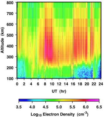
Fig. 1. EISCAT Svalbard Radar (ESR) electron density
observa-tions for 19 October 2002 (day 292). Altitude profiles of the iono-sphere above Longyearbyen are shown for a 24-h period; Neis color
coded on a logarithmic scale.
These data sets form the core of the high-latitude wind obser-vations that were used to create the climatological horizontal wind model (HWM), which is used extensively throughout the ionosphere-thermosphere community (Hedin et al., 1991 and 1996). At high-latitudes the wind variability is strongly dependent on geomagnetic history and the coverage of ob-servation is far from ideal. Both factors cause users of the HWM to have concerns when using it to represent specific events.
Most recently, the wind issue has become further compli-cated by studies which have shown that vertical neutral winds are often large and associated with gravity wave dynamics (Ford et al., 2003; Innis et al., 1999; Johnson et al., 1995; McEwen and Guo, 2003). The effects of such vertical winds can be considerable on the F-region (Sojka et al., 2001), be-cause the vertical wind can readily move plasma along the near vertical high-latitude magnetic field lines, rapidly af-fecting the plasma recombination rates and hence plasma density. The HWM, although having 3-D winds, does not include these large vertical winds generated during only spe-cial events.
In October 2002 the EISCAT Svalbard incoherent scatter radar created a historic first: a full month of continuous oper-ation, generating a high-resolution series of ionospheric pro-files over Longyearbyen, Norway. The expectation is to use this and future long-period ISR runs not just to validate the physics of high-latitude ionospheric models, but also as input data for assimilation models.
A model simulation of the ionosphere above Longyear-byen has been carried out for the month-long period of EIS-CAT data availability, using the observed values of F10.7, Kp, and IMF to drive the Utah State University Time De-pendent Ionospheric Model (TDIM) (Schunk, 1988; Sojka, 1989). As already alluded to, when the initial results were compared with the observations, a dramatic, almost inverse diurnal trend was found in the F-layer densities. The reso-lution of this discrepancy was not found in the normal high-latitude weather adjusting, i.e., magnetospheric convection or precipitation, but, rather surprisingly, in the neutral wind representation. Sections 2 and 3 introduce the month-long data set and the TDIM model with a detailed presentation for one particular day, 19 October 2002 (day 292). Section 4 describes the prevailing solar and geomagnetic conditions for the 30-day study period, which is then presented as a series of TDIM neutral wind sensitivity studies in Sect. 5. An interpre-tation of the diurnal F-region climatology at the Longyear-byen location is given in Sect. 6, and conclusions presented in Sect. 7.
2 EISCAT Svalbard Radar (ESR) observations
The EISCAT Svalbard Radar, an incoherent scatter radar lo-cated near Longyearbyen (78.2◦ geographic latitude, 15.8◦ geographic longitude), carried out continuous operations be-tween 4 October and 5 November 2002. The radar can switch rapidly between two antennas, one fully steerable and the other fixed along the local direction of the Earth’s magnetic field, but, for this experiment, the antennas were changed only every 64 s. The steerable antenna was directed sequen-tially between vertical and two positions at a lower elevation than the local field line, and to the east and west of it, each position being visited for 64 s in every 384-s cycle. Corre-sponding field-aligned data were recorded in every other 64-s interval. In the present study, only data from the field-aligned antenna have been used. The radar modulation scheme uses two identical, strong-condition, alternating codes transmitted on different frequencies. Clutter subtraction is implemented for all affected ranges and both codes cover the F-region peak, but with somewhat different overall range extents; the two are integrated together to produce fully decoded lag pro-files between altitudes of 90 and 1200 km. Before deriving the physical parameters required for this model comparison, the raw data were further post-integrated for 64 s.
Figure 1 shows the observed ESR electron density pro-files for 19 October 2002 (day 292). The electron density is color coded on a log10scale over three orders of magnitude. This day is reasonably typical of the month-long period, with an area of enhanced density between 08:00 and 10:00 UT, centered near magnetic noon at Longyearbyen. This corre-sponds to the geomagnetic cusp region. Note that local noon at Longyearbyen, (geographic longitude of 15.8◦) occurs at 11:00 UT which is significantly later than the density en-hancement. A second Ne enhancement, more extended and structured, extends from 16:00 to 22:00 UT. This spans the
0 2 4 6 8 10 12 14 16 18 20 22 24 100 200 300 400 500 600 700 800 Altitude (km) 0 2 4 6 8 10 12 14 16 18 20 22 24 UT (hr) 100 200 300 400 500 600 700 800 Altitude (km) 3.5 4.0 4.5 5.0 5.5 6.0 6.5
Log10 Electron Density (cm-3)
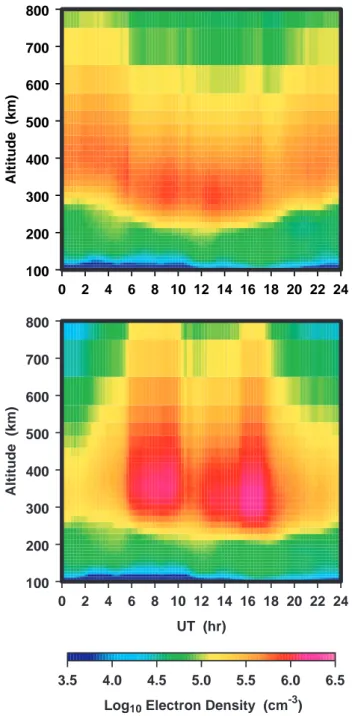
Figure 2 Fig. 2. TDIM simulations for the Longyearbyen location on 19
Oc-tober 2002, for the standard TDIM with HWM (top panel), and the TDIM with the neutral wind set to zero (bottom panel). Neis
dis-played in the same format as in Fig. 1.
evening to midnight magnetic local time sector. The region of lowest densities is encountered in the pre-noon, 01:00 to 05:00 UT period. This is a third “climatology” condition shared by almost all of the days in the month-long ESR ob-servation. The electron density profiles have somewhat dif-ferent peak heights as well. For convenience of presenting the entire month-long period, both for observations and mod-els, the electron density at 350 km will be used. From Fig. 1 it is evident that this height lies near the peak F-region den-sity at all UTs.
3 Time Dependent Ionospheric Model (TDIM)
The TDIM ionospheric model was initially developed as a mid-latitude, multi-ion ( NO+, O+2, N+2, and O+) model by Schunk and Walker (1973). The time-dependent ion conti-nuity and momentum equations were solved as a function of altitude for a corotating plasma flux tube, including di-urnal variations and all relevant E- and F-region processes. This model was extended to include high-latitude effects due to convection electric fields and particle precipitation by Schunk et al. (1975, 1976). A simplified ion energy equa-tions was also added, which was based on the assumption that local heating and cooling processes dominate (valid be-low 500 km). Flux tubes of plasma were folbe-lowed as they moved in response to the convection electric fields. The ad-dition of plasma convection and particle precipitation mod-els is described by Sojka et al. (1981a, b). Schunk and So-jka (1982) extended the ionospheric model to include ion thermal conduction and diffusion thermal heat flow. Also, the electron energy equation was included by Schunk et al. (1986), and consequently, the electron temperature is now rigorously calculated at all altitudes. The theoretical development of the TDIM is described by Schunk (1988), while comparisons with observations are discussed by So-jka (1989).
The standard form of the TDIM requires inputs for the neutral atmosphere, neutral wind, auroral precipitation, and convection electric field. These are represented by the MSIS-86 (Hedin, 1987), HWM (Hedin et al., 1991), Hardy oval (Hardy et al., 1987), and the Heppner and Maynard convection patterns (Heppner and Maynard, 1987), respec-tively. These drivers are empirical models that require the geomagnetic three-hourly Kpand Ap indices; the MSIS-86 and HWM models require the solar F10.7, and F10.7Aindices as well. These indices and IMF parameters are discussed in the next section. The convection patterns are based upon the interplanetary magnetic field (IMF) Byand Bzcomponents. Figure 2, top panel, is a TDIM Nesimulation for 19 October 2002, presented in the same format as the ESR observations in Fig. 1. This simulation does not convincingly reproduce the three major climatology features found in Fig. 1. Be-tween 08:00 and 10:00 UT there is only a weak enhancement, from 16:00 to 22:00 UT there is a minimum density rather than a second maximum, and between 01:00 and 05:00 UT the densities are large not small. In order to find the source of this model/data mismatch, a TDIM investigation was carried out with adjustments to the magnetospheric convection and precipitation drivers. Although different diurnal variations could be obtained, the three main characteristics were not reproduced. This eventually led to going back to the stan-dard TDIM configuration and simply turning off, setting to zero everywhere, the HWM neutral winds. Figure 2, bottom panel, shows the result of this simulation. Immediately ev-ident are major aspects of the three characteristics that are present in the observations. The contrast between high and low density features are now more acute and in the range ob-served. That the neutral wind has such a large influence in
194 J. J. Sojka et al.: Polar F-layer model-observation comparisons
the F-region density inside the polar cap came as a surprise. It is generally assumed that the horizontal neutral wind will have little or no effect on F-region densities in the polar cap, because the field lines are nearly vertical and the hor-izontal wind will not be effective in causing drifts upward or downward along the flux tube. But why then do we see such a large difference in model runs done with and without the HWM? The answer is found when considering the dom-inating role of plasma transport in the F-region. In fact, the HWM has its effect on the F-region at lower latitudes, and, an hour or several hours later, when this plasma flux tube is transported into the polar cap, it still retains some or all of the effect of the wind. In order to verify this, extra model runs were done, in which a) the horizontal wind was allowed only within 1000 km of Longyearbyen, and forced to be zero everywhere else, and b) the reverse, in which the horizontal wind was forced to be zero at all points within 1000 km of Longyearbyen, but normal elsewhere. The result of run “a” was nearly identical to the no-wind case, and “b” was nearly identical to the HWM standard case, showing that the effect of the wind in the polar cap is not local, but instead occurs at earlier times in other locations at lower latitudes.
This finding led to a sensitivity study of how the neu-tral wind, specifically its horizontal component affects the F-region in the winter polar cap. Hence, in the following month-long ESR observation-TDIM comparisons, a range of different horizontal wind patterns are used. Note in every case only the horizontal component of the neutral wind is used to induce vertical ion drift.
4 Prevailing solar, IMF, and geomagnetic conditions
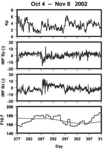
Figure 3 summarizes the solar, IMF, and geomagnetic activ-ity conditions during the month of ESR observations. No unusual solar, solar wind, or geomagnetic activity occurred. Three periods are readily associated with the IMF Bz mor-phology; from day 277 to 287 the IMF was southward, from 288 to 296 it was northward, and in the final period was near zero and slightly southward. During the first and third of these periods, Kp reached its largest values of 6 and was greater than 5 for several days. In the middle period, Kpwas significantly lower. The IMF By was near zero during the entire month, except for a negative excursion on days 287 and 288, the transition between periods 1 and 2. These same two days had the strongest northward IMF. The F10.7radio flux index showed ±12 units 27-day solar rotation modula-tion, with the average being 170. Given that the F-region po-lar cap generally has different convection during southward IMF (tongues of ionization and patches), than under north-ward IMF (Sun-aligned arcs) a difference in plasma struc-tures may be expected between period 2 and the others.
5 350 km Necomparison
Figure 4 presents the ESR-TDIM comparison for the month-long study period from 4 October (day 278) to 5 November
0 2 4 6 8 Kp -20 -10 0 10 20 IMF By ( γ ) -20 -10 0 10 20 IMF Bz ( γ ) 140 160 180 200 F10.7 277 282 287 292 297 302 307 312 Day 140 160 180 200 F10.7
Oct 4 -- Nov 8 2002
Figure 3 Fig. 3. Solar, IMF, and geomagnetic conditions during themonth-long study period. The bottom panel shows the F10.7 solar radio
flux index and its 81-day running average. The middle two panels show the IMF By(nT) and Bz(nT), while the top panel shows the
geomagnetic Kpindex.
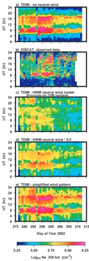
2002 (day 309). The observations have been averaged into 15-min bins; similarly the TDIM simulations produce output at 15-min intervals. In each panel of Fig. 4 the daily diur-nal variation is the vertical axis (UT) while the day of year is the horizontal axis. Four TDIM simulations are shown in Figs. 4, panels (a, c, d, and e). Each is described in the fol-lowing subsections. Overall, these four simulations provide a measure of the sensitivity of the TDIM F-region to the hor-izontal neutral wind, since this is the only difference between these otherwise standard TDIM simulations.
Figure 4, panel (b), shows the ESR month-long 15-min averaged Ne at 350 km. The three main characteristics de-scribed for Fig. 1 are still recognizable, but are modulated by the IMF Bzinterval. Hence, the northward period, days 288 to 296, has strong characteristics one and two, the enhanced densities between 08:00 to 10:00 UT and 16:00 to 22:00 UT. These two features are less well pronounced during the two southward periods. However, all three periods show the third characteristic, the appearance of the lowest densities from 01:00 to 05:00 UT.
5.1 Standard TDIM (HWM Wind)
The standard TDIM results for the electron density at 350 km are shown in Fig. 4, panel (c). Comparison with the ESR ob-servations in panel b reveals large-scale disagreements, both in dynamic range and overall structure. The TDIM does not have the lowest densities between 01:00 and 05:00 UT; in fact, for southward period 1, day 277 to 286, some of the highest densities are found during this time. The ESR data shows a high density “ridge” between 17:00 and 22:00 UT, the TDIM shows a distinct depletion between 17:00 and 19:00 UT. Other very large differences are apparent for peri-ods 2 and 3 as well, specifically that the low and high den-sity characteristics defined for the observations and seen in Figs. 1 and 4, panel (b) are almost inverted in the model sim-ulation.
5.2 TDIM with no wind
Figure 4, panel (a), shows the TDIM electron density at 350 km for the case when the neutral wind was set to zero. Climatologically, the improved agreement with the ESR ob-servations is remarkable. The low densities occur during the same time period, 01:00–05:00 UT; the noon-time high den-sity structures near 08:00 UT correlate in UT and also show a similar monthly morphology with the highest densities be-ing in period 2, days 288 to 296. However, the second high density period occurs about 3 to 4 h earlier in this TDIM sim-ulation. The TDIM shows the two high density features con-tinuously over the month long period with some day-to-day modulation. In contrast the observations show that the day-to-day modulation breaks up these two high density ridges; only between days 283 and 296 is the 08:00 to 10:00 UT high density ridge continuous. Both the ESR and TDIM show densities between 10:00 UT to 16:00 UT that are higher than those between 22:00 and 05:00 UT.
5.3 TDIM with the HWM wind scaled by 0.5
Figure 4 panel (d) shows the TDIM electron density at 350 km when the TDIM HWM input was scaled by 0.5. This simulation produces results approaching the no-wind case, panel (a). However, the 22:00 to 06:00 UT low density re-gion is not low enough, compared to the observations shown in panel (b). In general, the “no wind” and “half HWM” simulations have the 08:00 to 10:00 UT enhanced density feature, but it is too high and extended in UT.
5.4 TDIM with a simplified wind pattern
During the development phase of the TDIM in the late 1970s and early 1980s a simple horizontal wind description was used (Sojka et al., 1981a, b). This wind pattern was adopted from the work of Murphy et al. (1976) and had the features of being zero in sunlight and whenever a downward induced vertical ion drift was computed. In the night sector the hor-izontal wind was set to 200 m/s everywhere in a direction anti-sunward towards 01:00 MLT. The result of using this
5.25 5.50 5.75 6.00 6.25
Log10 Ne 350 km (cm-3)
a) TDIM - no neutral wind
0 4 8 12 16 20 24 UT (hr)
b) EISCAT observed data
0 4 8 12 16 20 24 UT (hr)
c) TDIM - HWM neutral wind model
(Previously the TDIM standard)
0 4 8 12 16 20 24 UT (hr)
d) TDIM - HWM neutral wind * 0.5
0 4 8 12 16 20 24 UT (hr)
e) TDIM - simplified wind pattern
275 280 285 290 295 300 305 310 315 Day of Year 2002 0 4 8 12 16 20 24 UT (hr) Figure 4 Fig. 4. Electron densities at Longyearbyen, at 350 km altitude,
dur-ing the month-long study period in October-November 2002. Pan-els (a, c, d, e) are TDIM simulations; panel (b) shows ESR observa-tions. Daily UT variations are displayed vertically while day-to-day differences are shown horizontally. The four TDIM simulations dif-fer only in their neutral wind input.
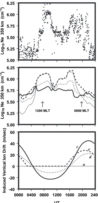
196 J. J. Sojka et al.: Polar F-layer model-observation comparisons 5.00 5.25 5.50 5.75 6.00 6.25 Log 10 Ne 350 km (cm -3 ) 1200 MLT 0000 MLT 0000 0400 0800 1200 1600 2000 2400 UT -40 -20 0 20 40 60
Induced Vertical Ion Drift (m/sec)
c d e a 5.00 5.25 5.50 5.75 6.00 6.25 Log 10 Ne 350 km (cm -3 )
Figure 5
Fig. 5. Comparisons of electron densities at 350 km for day 292.
ESR observed Neis shown in the top panel, with four TDIM
simu-lation results in the middle panel, and the induced vertical ion drifts for the four TDIM simulations in the bottom panel. The letters (a, c, d, e) correspond to the labels in Fig. 4: (a) no wind, (c) standard HWM, (d) half HWM, and (e) for simplified wind.
simple neutral wind model in the TDIM is shown in Fig. 4 panel (e); the results are quite favorable and are comparable to the no-wind and half-HWM cases. However, on certain days, i.e. 282 through 286, the simulation has generated very large densities between 22:00 and 05:00 UT, a period when the densities are observed to be low.
5.5 Horizontal wind Induced Vertical Ion Drifts (IVID)
The four model simulations in Fig. 4 are graphically quite different and show a range of diurnal trends which range from being in good agreement with the observations, panels a and e, to being poorly out of phase, panel c. A quantitative view of these diurnal differences and their IVID differences is shown in Fig. 5 for 19 October 2002 (day 292). The top panel shows the ESR Neat 350 km; the middle panel shows Ne at 350 km for the four simulations, and the lower panel shows the corresponding IVIDs for the four simulations. A line style pattern is used to distinguish between the four mod-els; they are labeled with the panel letters from Fig. 4. Fig-ure 5, top panel, shows the usual ESR three main featFig-ures; first, high densities from 08:00 to 10:00 UT; second, a fur-ther Neenhancement spread from 16:00 to 22:00 UT which is heavily structured, and the third, low densities from 01:00 to 08:00 UT. In the middle panel only the thin line which corresponds to the “no-wind” TDIM simulation has all three features, but arguably the three features are not perfectly aligned in UT with the observations. The poorest agreement is found for the dark solid line which is the standard TDIM with the HWM wind. This simulation has only a weak mod-ulation over the 24-h period with its lowest density occur-ring at 18:00 UT just when the observations show the second peak. The other two simulations lie between these two ex-tremes.
Quantitatively the difference between the four simulations is more than a factor of 2 with the diurnal modulation in the no-wind simulation having Ne at 350 km ranging from 2×105cm−3at 01:00 UT to 1.7×106cm−3at 16:00 UT. An indication of how the IVID is causing these differences can be obtained from the lower panel in Fig. 5; note, however, that these IVID values correspond to the Longyearbyen lo-cation where the horizontal wind is not at its most effective. Nonetheless, between 05:00 and 16:00 UT, approximately centered around local noon, the IVID is downward for the standard TDIM (dark solid line). This downward IVID on the dayside causes the F-layer to be depressed in both alti-tude and density; the standard TDIM density is more than a factor of 4 lower for the two observed peak features. As a fur-ther note, the fact that the peak height (hmF2) is depressed by the downward IVID could seem to suggest that 350 km is far above the peak, and hence we are merely seeing lower top-side densities; however, the altitude profiles shown in Fig. 2, lower panel, clearly show this argument to be secondary. The enhanced IVID at the other UTs for the standard TDIM have a relatively smaller role, but they do lead to maintenance of the nighttime density and hence this simulation shows a very small day-night modulation in Neat 350 km.
6 Polar cap morphology
The model results presented in Sect. 5 indicate the sensitivity of the polar cap F-region to the horizontal neutral winds at lo-cations far from the observer. In this section we examine the
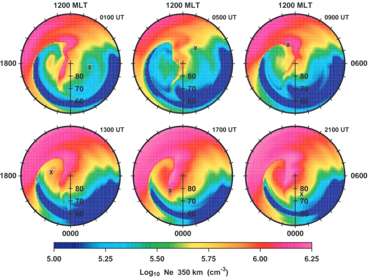
5.00 5.25 5.50 5.75 6.00 6.25 Log10 Ne 350 km (cm-3) 1800 1200 MLT 80 70 60 0100 UT XX 1200 MLT 80 70 60 0500 UT XX 0600 1200 MLT 80 70 60 0900 UT XX 0000 1800 80 70 60 1300 UT XX 0000 80 70 60 1700 UT XX 0000 0600 80 70 60 2100 UT XX
Figure 6
Fig. 6. Six snapshots of simulated electron density at 350 km at 4 hourly intervals from the no-wind TDIM study for 8 October 2002 (day
281). Each panel shows the logarithm of electron density, as well as an X marking the location of Longyearbyen in an MLT-magnetic latitude coordinate system.
morphological regions associated with the three main density features identified in the observations. Figure 6 shows a se-ries of snapshots, 8 October 2002 (day 281), of the simulated electron density at 350 km for the “no wind” TDIM simula-tion. Each snapshot shows the electron density poleward of 50◦magnetic latitude in a polar magnetic local time coordi-nate system. In each panel an X represents the Longyear-byen location at that UT. The panels are separated in UT by 4 h. The usual polar cap density structures can be seen in these dial plots: the tongue of ionization (TOI), patches, po-lar holes, and the noon sector daylight enhancement. Near 09:00 UT (top row, right panel) Longyearbyen is in the mag-netic noon sector cusp region, and intersects the TOI plasma flow from lower latitudes to the cusp and into the polar cap. This corresponds to the first feature, i.e. the enhanced den-sity observed between 08:00 and 10:00 UT. From 01:00 to 05:00 UT, top left and middle panels, Longyearbyen is in the morning sector polar cap which has relatively lower
densi-ties; this density depletion region is a polar hole. In Fig. 4, panel (b), it is evident that this polar hole is consistently en-countered at Longyearbyen and is the third of the density features previously enumerated.
As Longyearbyen traverses the night sector it again crosses the TOI around 17:00 UT. This second high density feature is modeled to be tightly centered near 17:00 UT while the ob-servations show an extended region from 16:00 to 22:00 UT. In this case the transport across the entire polar cap has oc-curred and would be heavily dependent upon the details of high-latitude convection over several hours. The mismatches in UT and UT spread, as well as fine structuring in density, are likely to be attributable to the use of an empirical con-vection model that poorly represents the true concon-vection for a specific day.
198 J. J. Sojka et al.: Polar F-layer model-observation comparisons
7 Conclusion
In this study we have used a month-long EISCAT Svalbard Radar observation for comparison with the TDIM model, and we have drawn the following conclusions:
– Unexpectedly, the polar F-region at Longyearbyen is very sensitive to the horizontal neutral wind.
– The 1991 HWM produces induced vertical ion drifts in the TDIM which result in F-region densities at 350 km that are morphologically out of phase with observations.
– A zero neutral wind produces induced vertical ion drifts in the TDIM which lead to much better agreement with observations in the F-region.
– Variations of the neutral wind can create factors of 2 variations in the electron density.
– The three main climatology features observed by ESR and discussed in Sect. 2, have been correlated with well-known polar ionosphere features as follows: 1) between 08:00–10:00 UT the magnetic noon cusp region with the TOI entering the polar cap; 2) between 16:00–22:00 UT Longyearbyen transverses the nightside remnants of the TOI and patch structures; and 3) from 01:00–05:00 UT Longyearbyen is located in a polar hole.
– Unfortunately none of the fine structure weather fea-tures can be simulated with the empirical drivers used as input to the TDIM, although the general differences be-tween northward IMF (days 288 to 296) and southward IMF (the remaining days) are qualitatively reproduced.
The month-long ESR database has sufficient time resolution and duration to investigate diurnal dependences, as well as month-long morphologies. A follow-up study will be under-taken to determine how much neutral wind data was observed by FPIs in the high-latitude regions; if sufficient horizontal wind measurements are available, it will be possible to carry out a further TDIM simulation in which the induced verti-cal ion drifts are based on the observed horizontal neutral winds. A TDIM study is under way to compare model runs at mid-latitudes with the Millstone Hill ISR month-long data set taken at the same time as the ESR observations, to see if the “no wind” improvement found in the polar cap will also hold true at a location equatorward of the cusp.
Acknowledgements. This research was supported by NASA Grant
NAG5-11880 and NSF Grant ATM-0000171 to Utah State Univer-sity. EISCAT is an International Association supported by Finland (SA), France (CNRS), the Federal Republic of Germany (MPG), Japan (NIPR), Norway (NFR), Sweden (VR) and the United King-dom (PPARC).
Topical Editor M. Lester thanks E. Griffin and J. Makela for their help in evaluating this paper.
References
Ford, E. A. K., Aruliah, A. L., Griffin, E. M., McWhirter, I., Ayl-ward, A. D., and Kosch, M. J.: Meso-Scale measurements of the thermosphere using co-located FPIS and EISCAT radars (Ab-stract), Geophysical Research Abstracts, 5, 10 017, 2003. Hardy, D. A., Gussenhoven, M. S., Raistrick, R., and McNeil, W. J.:
Statistical and functional representations of the pattern of auroral energy flux, number flux, and conductivity, J. Geophys. Res., 92, 1 275–12 294, 1987.
Hays, P. B., Killeen, T. L., Spencer, N. W., Warton, L. E., Roble, R. G., Emery, B. A., Fuller-Rowell, T. J., Rees, D., Frank, L. A., and Craven, J. D.: Observations of the dynamics of the polar thermosphere, J. Geophys. Res., 89, 5597–5612, 1984.
Hedin, A. E.: MSIS-86 thermospheric model, J. Geophys. Res., 92, 4649–4662, 1987.
Hedin, A. E., Spencer, N. W., Biondi, M. A., Burnside, R. G., Her-nandez, G., and Johnson, R.M.: Revised global model of ther-mospheric winds using satellite and ground-based observations, J. Geophys. Res., 96, 7657–7688, 1991.
Hedin, A. E., Fleming, E. L, Manson, A. H., Schmedline, F. J., Avery, S. K., Clark, R. R., Frank, S. J., Fraser, G. J., Tsuda, T., Vial, F., and Vincent, R. A.: Empirical wind model for the upper, middle and lower atmosphere, J. Atmos. S.-P., 58, 1421–1447, 1996.
Heppner, J. P. and Maynard, N. C.: Empirical high-latitude electric field models, J. Geophys. Res., 92, 4467–4489, 1987.
Innis, J. L., Greet, P. A., Murphy, D. J., Conde, M. G., and Dyson, P. L.: A large vertical wind in the thermosphere at the auroral oval/polar cap boundary seen simultaneously from Mawson and Davis, Antarctica, J. Atmos. S.-P., 61 (14), 1047–1058, 1999. Johnson, F. S., Hanson, W. B., Hodges, R. R., Coley, W. R.,
Carig-nan, G. R., and Spencer, N. W.: Gravity waves near 300 km over the polar caps, J. Geophys. Res., 100, 23 993–24 002, 1995. Killeen, T. L., Hays, P. B., Spencer, N. W., and Wharton, L. E.:
Neutral winds in the polar thermosphere as measured from Dy-namics Explorer, Geophys. Res. Lett., 9, 957–960, 1982. Killeen, T. L., Smith, R. W., Hays, P. B., Spencer, N. W.,
Whar-ton, L. E., and McCormac, F. G.: Neutral winds in the high-latitude winter F-region: Coordinated observations from ground and space, Geophys. Res. Lett., 11, 311–314, 1984.
Killeen, T. L., Roble, R. G., Smith, R. W., Spencer, N. W., Meri-wether Jr., J. W., Rees, D., Hernandez, G., Hays, P. B., Cogger, L. L., Sipler, D. P., Biondi, M. A., and Tepley, C. A.: Mean neu-tral circulation in the winter polar F-region, J. Geophys. Res., 1633–1649, 1986.
McEwen, D. J. and Guo, W.: Vertical winds in the central polar cap (Abstract), Geophysical Research Abstracts, 5, 07336, 2003. Murphy, J. A., Bailey, G. J., and Moffett, R. J.: Calculated daily
variations of O+and H+at mid-latitudes, J. Atmos. Terr. Phys, 38, 351–364, 1976.
Schunk, R. W.: A mathematical model of the middle and high-latitude ionosphere, Pur. A. Geoph., 127, 255–303, 1988. Schunk, R. W. and Sojka, J. J.: Ion temperature variation in the
day-time high-latitude F region, J. Geophys. Res., 5169–5183, 1982. Schunk, R. W. and Walker, J. C. G.: Theoretical ion densities in the lower ionosphere, Planetary and Space Sciences, 21, 1875–1896, 1973.
Schunk, R. W., Raitt, W. J., and Banks, P. M.: Effect of electric fields on the daytime high-latitude E and F regions, J. Geophys. Res., 80, 3121–3130, 1975.
Schunk, R. W., Banks, P. M., and Raitt, W. J.: Effect of elec-tric fields and other processes upon the nighttime high-latitude F layer, J. Geophys. Res., 81, 3271–3282, 1976.
Schunk, R. W., Sojka, J. J., and Bowline, M. D.: Theoretical study of the electron temperature in the high-latitude ionosphere for solar maximum and winter conditions, J. Geophys. Res., 91, 12 041–12 054, 1986.
Sojka, J. J.: Global scale, physical models of the F region iono-sphere, Rev. Geophys., 27, 371–403, 1989.
Sojka, J. J., Raitt, W. J., and Schunk, R. W.: Theoretical predictions for ion composition in the high-latitude winter F region for solar minimum and low magnetic activity, J. Geophys. Res., 86, 2206– 2216, 1981a.
Sojka, J. J., Raitt, W. J., and Schunk, R. W.: A theoretical study of the high-latitude winter F region at solar minimum for low magnetic activity, J. Geophys. Res., 86, 609–621, 1981b. Sojka, J. J., Schunk, R. W., David, M., Innis, J. L., Greet, P. A., and
Dyson, P. L.: A theoretical model study of F-region response to high-latitude neutral wind upwelling events, J. Atmos. S.-P., 63, 1571-1584, 2001.