Accelerated atomistic prediction of structure, dynamics and material properties in molten salts

(1)

Accelerated atomistic prediction of structure, dynamics and material

properties in molten salts

by

Stephen Tsz Tang Lam

B.A.Sc., Chemical Engineering, 2013

University of British Columbia M.S., Nuclear Science and Engineering, 2017

Massachusetts Institute of Technology

Submitted to the department of Nuclear Science and Engineering in partial fulfillment of the requirements for the degree of Doctor of Philosophy in Nuclear Science and Engineering

at the

Massachusetts Institute of Technology September 2020

Signature of Author:

Stephen T. Lam Department of Nuclear Science and Engineering July 13, 2020

Certified by:

Ronald G. Ballinger Professor of Nuclear Science and Engineering and Professor of Materials Science and Engineering Thesis Co-supervisor

Certified by:

Ju Li Battelle Energy Alliance Professor of Nuclear Science and Engineering and Professor of Materials Science and Engineering Thesis Co-supervisor

Certified by:

Charles W. Forsberg Principal Research Scientist, Nuclear Science and Engineering Thesis Reader

Accepted by:

Ju Li Battelle Energy Alliance Professor of Nuclear Science and Engineering and Professor of Materials Science and Engineering Chair, Department Committee on Graduate Students

(2)

(3)

Accelerated atomistic prediction of structure, dynamics and material

properties in molten salts

by

Stephen Tsz Tang Lam

Submitted to the Department of Nuclear Science and Engineering On July 13, 2020, in partial fulfillment of the

requirements for the degree of

Doctor of Philosophy in Nuclear Science and Engineering

Abstract

Various advanced nuclear reactors including fluoride high-temperature salt-cooled reactors (FHRs), molten salt reactors (MSRs) and fusion devices have proposed to use molten salt coolants. However, there remain many uncertainties in the chemistry, dynamics and physicochemical properties of many salts, especially over the course of reactor operation, where impurities are introduced, and compositional and thermodynamic changes occur.

Density functional theory (DFT) and ab initio molecular dynamics (AIMD) were used for property, structure and chemistry predictions for a variety of salts including LiF, KF, NaF, BeF2, LiCl, KCl, NaCl,

prototypical Flibe (66.6%LiF-33.3%BeF2), and Flinak (46.5%LiF-11.5NaF-42%KF). Predictions include

thermophysical and transport properties such as bulk density, thermal expansion coefficient, bulk modulus, and diffusivity, which were compared to available experimental data. DFT consistently overpredicted bulk density by about 7%, while all other properties generally agreed with experiments within experimental and numerical uncertainties. Local structure was found to be well predicted where pair distribution functions showed similar first peak distances (+ 0.1 Å) and first shell coordination numbers (+ 0.4 on average), indicating accurate simulation of chemical structures and atomic distances. Diffusivity was also generally well predicted within experimental uncertainty (+20%).

Validated DFT and AIMD methods were applied to study tritium in prototypical salts since it is an important corrosive and diffusive impurity found in salt reactors. It was found that tritium species diffusivity depended on its speciation (TF vs. T2), which was related to chemical structures formed in Flibe

and Flinak salts. Further, predictions allowed comparison with and interpretation of past contradictory experimental results found in the literature.

Lastly, robust neural network interatomic potentials (NNIPs) were developed for LiF and Flibe. The LiF NNIP accurately reproduced DFT calculations for pair interactions, solid LiF and liquid molten salt. The Flibe NNIP was developed for molten salt at the reactor operating temperature of 973K and was found to reproduce local structures calculated from DFT and showed good stability and accuracy during extended MD simulation. Ab initio methods and NNIPs can play a major role in advanced reactor development. Combined with experiments, these methods can greatly improve fundamental understanding and accelerate materials discovery, design and selection.

Thesis Co-supervisor: Ronald G. Ballinger

Title: Professor of Nuclear Science and Engineering, and Materials Science and Engineering

Thesis Co-supervisor: Ju Li

Title: Battelle Energy Alliance Professor of Nuclear Science and Engineering, and Materials Science and Engineering

(4)

(5)

Thesis Acknowledgements

Firstly, I would like to thank my advisors Professor Ron Ballinger, Dr. Charles Forsberg and Professor Ju Li. Each of them has provided tremendous insight and support. Professor Ballinger and Dr. Forsberg were also my master’s thesis advisors and I have greatly enjoyed our conversations over the years. Further, I am grateful for their unwavering attentiveness and investment in my work and personal development. Professor Ju Li’s technical guidance, kindness and career advice have been invaluable to me, and I am certain that I will continue to benefit from his mentorship for many years going forward. Additionally, I would like to thank Professor Mingda Li for agreeing to be my committee chair and Brandy Baker for agreeing to be the MC for my defense. As well, I would like to acknowledge the Shanghai Institute of Nuclear and Applied Physics at the Chinese Academy of Sciences for supporting this work.

I would like to acknowledge everyone who contributed intellectually to my work and skill development. This includes the computational material science group at Bosch, which consisted of Jonathan Mailoa, Boris Kozinsky, Mordechai Kornbluth, Georgy Samsonidze and Soo Kim. They gave me wonderful opportunities to learn and I have benefitted from working with them. As well, I would like to thank Professor Raluca Scarlat, Professor Jinsuo Zhang and scientists at the MIT nuclear reactor laboratory including Dave Carpenter, Guiqiu (Tony) Zheng and Kieran Dolan for the many wonderful discussions and collaborations. I would like to thank Professor Koroush Shirvan for helping me prepare for my qualifying exams and for being great to work with during the Reactor Technology Course (RTC). As well, I would like to thank Professor Matteo Bucci with whom I had my first teaching assistantship. I deeply admire his commitment to students and he has significantly influenced my own teaching and career. Lastly, I would like to thank all the members in Professor Li’s lab for our many fruitful exchanges and meetings. This group includes Qingjie Li, Frank Shi, Haowei Xu, David Bloore, and many more.

I am thankful for my office mates Lucas, Nestor, Robbie and Patrick who created an entertaining environment to work in over the last few years, my roommates Guillaume and Shikhar, friends in the department including Artyom, Malik and Sam, RTC TAs Sterling, Chloe, and Anna, and many friends from the University of British Columbia and back home. As well, I would like to acknowledge department administrators Brandy, Pete, Anne, and Lisa for their support. They have all made life easier and much more enjoyable during my graduate studies.

Most importantly, I would like to thank my mother, father, siblings Amy, Janet, Sherry and Sharon, and my fiancé Emily. Without all of them, this work would not have been possible.

(6)

List of Tables

Table 4.1 Output of reaction search in HF + F2 system. ... 61

Table 4.2: Output of reaction search in HF + MgO where * denotes surface. ... 62

Table 5.1: Experimental versus calculated bulk modulus. The simulation temperatures for LiCl, NaCl, KCl, LiF were 1053, 1301, 1212 and 1318 K compared to interpolated data from experimental data. *NaF experimental temperature was 1395K while simulation temperature was 1550 K and KF experimental temperature was 1244 K while simulation temperature was 1310 K [171][172]. ... 70

Table 5.2: Comparison between experimental and simulated thermal expansion coefficients... 71

Table 5.3: First peak radius (Å) and coordination number for binary molten halides. Simulations were performed to match experimental temperatures for BeF2, KF, LiF and NaF in which temperatures were 973K, 1143K, 1148K and 1273K respectively. For chlorides KCl, LiCl and NaCl, the simulation temperatures were 1200K, 1040K, and 1300K respectively. The simulation temperatures for KCl, LiCl, and NaCl were 1073, 958 and 1148K respectively [175][176][177]. ... 74

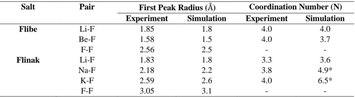
Table 5.4: First peak radii and coordination numbers for Flibe and Flinak. Flibe temperature was 973 K. Simulation temperature for Flinak is 973 K and experimental temperature 793 K. ... 75

Table 5.5: First peak radius and coordination number of T-F in Flibe and Flinak at 973K (design temperature for typical reactor) for TF and T2. The coordination number is determined by integration of the first shell of the RDF. Coordination numbers are excluded for T2 due to lack of clear solvation shell... 84

Table 5.6: Tritium reactions of TF in Flibe found during NVT simulation. ... 87

Table 5.7: AIMD diffusivities of tritium as TF and T2 in Flibe. ... 90

Table 5.8: AIMD diffusivities of tritium as TF and T2 in Flinak. ... 92

Table 6.1: Summary of symmetry functions used for neural network input features. The example below is shown for a Li central atom. Same parameters are used for F or any other elements in the system. ... 95

Table 6.2: Calculated surface energies from DFT versus neural networks. ... 98

Table 6.3: Energy and forcers training error for different phases of LiF. ... 100

Table 6.4: Neural network potential energy and force mean average error (MAE) for training, validation and test data sets. ... 102

Table 7.1: Recommended thermophysical properties and 95% confidence uncertainties for density (𝜌), viscosity (𝜇), heat capacity (𝐶𝑃) and thermal conductivity (𝑘) [6]. ... 108

(9)

List of Figures

Figure 1.1: FHR system level overview. ... 12

Figure 1.2: PB-FHR pebble fuel element [9]. ... 13

Figure 1.3: Redox potentials of various redox couples as function of temperature in fluoride salts. Solid line: metal oxidation at 𝑎M+ of 10−6; Dotted line: oxidation of reductants. HF/H2 represents the mole ratio of HF/H2 at 1 atm total pressure [19][20]. ... 16

Figure 1.4: MSR program approach to screening and justifying candidate MSR salts. ... 19

Figure 1.5: Fission product classes identified during MSRE operation highlighted by type in the Periodic table of elements (below) and the fission-yield curve (above). ... 20

Figure 1.6: a) ARC fusion system perspective view, b) Flibe fusion blanket surrounding plasma. ... 23

Figure 1.7: Nuclear reactions with Flibe salt [35]. ... 24

Figure 3.1: Radial symmetry functions a) varying Gaussian position 𝑅s and b) varying Gaussian width 𝜂. ... 41

Figure 3.2: Angular symmetry function with a) varying angular shift 𝜃s and b) varying width 𝜁. ... 42

Figure 3.3: Structure of a feedforward neural network. ... 44

Figure 3.4: Calculation of total energy and forces using high-dimensional neural networks. ... 45

Figure 4.1: Radial distribution functions of LiF and BeF2 [69]. ... 53

Figure 4.2: Raw signals from an Al2O3 + HF simulation of 2200 fs with 1 fs per time step at 1000K. Each colored line represents a different molecule that is generated. ... 57

Figure 4.3: Example of an interaction that creates a false signal. Green is aluminum, red is oxygen, pink is fluorine and white is hydrogen. ... 58

Figure 4.4: Schematic of hidden Markov model where 𝐸(𝑡) represents the observed state, and 𝑋(𝑡) represents the hidden state at time t. The state at 𝑋 is directly dependent on the state preceding it and state 𝐸(𝑡) is dependent on 𝑋(𝑡) [142]. ... 58

Figure 4.5: Example of signal filtering of a true adsorption of HF on an Al2O3 surface. ... 59

Figure 4.6 Reaction of H2 and F2 with a) the reactants, b) reactant intermediate during the reaction, and c) the product of the reaction ... 62

Figure 4.7: Adsorption and dissociation of HF on MgO surface: a) gaseous HF over MgO surface, b) adsorbed HF, c) dissociated HF on MgO surface. ... 63

Figure 5.1: Equation of state (EOS) fitting for binary fluoride using ab initio molecular dynamics NVT data, LiCl at 1053K. EOS fitting for LiF, KF, NaF, KCl and NaCl is found in Appendix A. ... 65

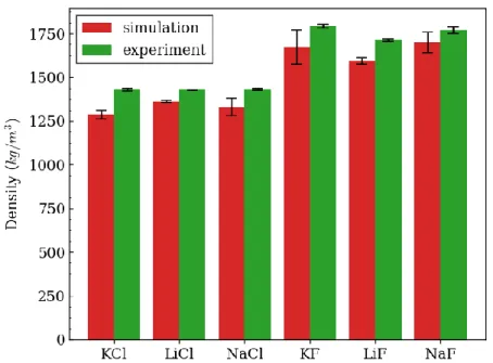
Figure 5.2: Bulk density calculated from simulation and experiment for binary chlorides and fluorides. The experimental temperatures matched simulation at 1212, 1053, 1301, 1310, 1318, and 1550 K for KCl, LiCl, NaCl, KF, LiF, and NaF, respectively. ... 66

Figure 5.3: Total pressure at the experimental density for standard KS-DFT compared to DFT with D3 dispersion correction. ... 68

Figure 5.4: Radial distribution functions (From left to right, top to bottom) for KF, KCl, LiF, LiCl, NaF, NaCl, BeF2 including cation-anion, anion-anion, and cation-cation pair functions. ... 73

Figure 5.5: Radial distribution functions for a) Flibe at 973K and b) Flinak at 973K. ... 75

Figure 5.6: Ion diffusivities of different binary molten salts. ... 77

(10)

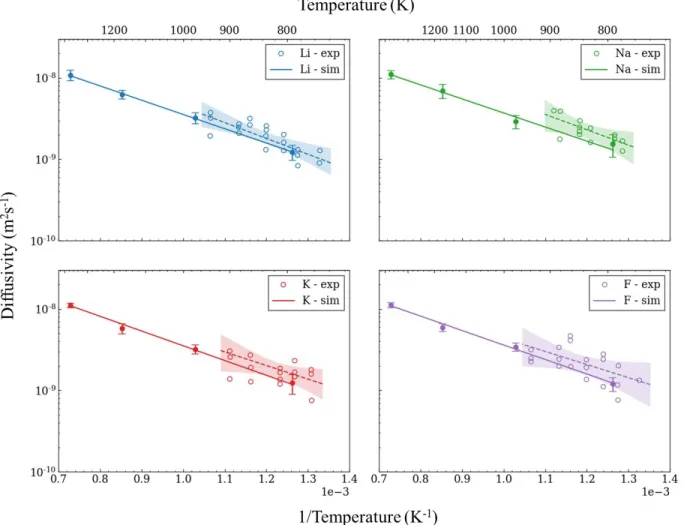
Figure 5.8: Self diffusivity from 775K to 1300K of a) fluorine and b) lithium in eutectic composition of LiF-KF. Experimental data from Sarou-Kainan et al [190]. ... 79 Figure 5.9: Self-diffusivity of ions in Flinak compared to experimental data. ... 80 Figure 5.10 Self diffusivity of Li and F ions in Flibe compared to other studies [190][151][194][195]. ... 82 Figure 5.11: Radial distribution functions and running coordination number of T-F for T2 and TF in a)

Flibe at 973K and b) Flinak at 973K. The coordination number is calculated by

integration of the RDF. ... 84 Figure 5.12: T+_{ion in Flibe, interatomic distance between tritium and fluorine atoms in the solution. The}

hopping T+_{occurs in sequence 1-5 shown below. Step 1 to 2 clearly show the existence}

of the HF2- complex where the T+ is bound to two fluorine atoms. Simulation

temperature is 973K. ... 85 Figure 5.13: a) Tritium molecules in Flibe, b) fraction of each molecule at 973K, 1173K, and 1373K. ... 86 Figure 5.14: a) Tritium molecules in Flinak, b) fraction of each molecule at 973K, 1173K, and 1373K. . 87 Figure 5.15: Tritium diffusivity in Flibe. Experiments versus simulation. The shaded region represents the error in approximation [200][199][201]. ... 90 Figure 5.16: Hydrogen diffusion in three experiments. The highlighted region represents the 95%

confidence interval from regression of the collected data [203][204][202]. ... 91 Figure 6.1: DFT versus NN predictions for a) pair interactions for Li-F, Li-Li and F-F and b) Equation of

state for bulk B1 phase LiF [213] at 0K. ... 96 Figure 6.2: LiF surfaces with different surface terminations and 1:1 Li:F stoichiometry. ... 98 Figure 6.3: Graphical representation of LiF as a) solid crystalline bulk B1 phase, b) semi-amorphous

crystal near melting point at 1120 K and c) molten LiF at 1200 K. ... 99 Figure 6.4: LiF neural network test errors. a) Parity plot for amorphous, solid and liquids calculated from

neural networks and AIMD, b) normalized probability density function of energy errors, and c) force parity plot for all calculations. ... 100 Figure 6.5: Neural network versus ab initio prediction of a) potential energies and b) forces. ... 101 Figure 6.6: Neural network trajectory with each meta time step representing 2 ps. Configurations are

recalculated in DFT and the ab initio energies are compared. ... 102 Figure 6.7: Neural network potential and DFT radial distribution functions obtained for Be-F, Li-F and

F-F pairs in F-Flibe. ... 103 Figure 6.8: a) CPU-hours for 1000 MD time steps versus number of atoms, b) computational speedup for

Flibe system with 2457 atoms. The black dashed line represents ideal efficiency. ... 105 Figure 7.1: Removal efficiency of tritium permeator with cylindrical flow tubes, calculated with

diffusivities taken from different sources [200][202]. ... 112 Figure 7.2: Expected impurities in FHRs. ... 113

(11)

Chapter 1. Introduction

1.1. Molten salts in nuclear applications

Various next generation nuclear reactors, including a variety of fusion devices, have proposed the use of molten salt coolants [1][2][3]. Molten salts offer substantially higher heat capacities and boiling points than water coolants. This allows operation at high temperature and low pressure, which increases thermodynamic efficiency and reduces containment safety demands. As a result, the use of molten salts can enable design simplification, increase economic value, and potentially provide inherent safety via passive heat rejection [4]. As such, molten salt-cooled reactors have garnered attention domestically and internationally, with several federally supported agencies and commercial companies performing research and development in this area [5][6]. In order to build and operate any salt-cooled reactor however, the evolution of salt chemistry and chemical properties of molten salts during operation must first be understood. In this chapter, the three main classes of advanced reactors that will use salts are described along with their chemical considerations. These systems include (1) fluoride-salt-cooled high-temperature reactors (FHRs) using clean salt and solid fuel [2], (2) molten salt reactors (MRSs) with fuel dissolved in salt [7], and (3) fusion reactors with molten salt blankets [3].

Central to development of these power systems, is a fundamental understanding of the physical and chemical properties of the salt. Section 1.5 describes the focus of this thesis in understanding structure, dynamics and properties of these salts. The structure and dynamics is fundamental to all research areas, and understanding this is key to gaining insight into salt phase transitions, viscosity, thermal conductivity, volatility, solubility, corrosion and more—the engineering properties required for plant design. The goal of this work is to demonstrate and accelerate atomistic simulation methods that provide such insights in molten salt systems of varying compositional complexity. The work involves applying a combination of electronic structure methods (DFT), molecular dynamics (MD), and machine learning methods to predict the chemistry, structure and dynamics of molten salts and comparing

predictions with experimental observables. This elucidates deeper chemical understanding and provides a basis for continued exploration with predictive computational methods.

(12)

1.2. Fluoride high-temperature salt-cooled reactors (FHRs)

1.2.1. FHR system overview

The FHR is a solid-fuel fission reactor with molten salt coolant. This reactor concept, originally proposed by Forsberg, Peterson and Pickard [8], combines emergent technologies including a low vapor-pressure fluoride molten salt, structurally robust graphite coated-particle fuel, and an open-air Brayton cycle. A system overview of the FHR is provided in Figure 1.1, which shows the primary system coupled to the Brayton cycle. In this system, heat is transferred from primary salt operating at 600 – 700o_{C and}

atmospheric pressure to compressed atmospheric air at 419o_{C and 18.6 bar via the coiled tube air heaters}

(CTAHs). One feature unique to FHRs that is shown in the diagram is the gas co-firing capability whereby natural gas is injected and combusted in a gas turbine. This allows for better load following on the grid and plant optimization by allowing the purchase of gas when costs are low to produce electricity at a lower cost per megawatt (MW). This provides a more flexible power output with peaking capabilities able to bring the reactor/system from the normal operating power of 100 MWe to 242 MWe. The outlet stream from the gas turbine enters the heat-recovery steam generator, which can power a Rankine cycle to generate more electricity or provide process heat. In combination, these have the effect of increasing the thermal efficiency to 66.4 % and increasing plant revenues by more than 40% [9][10][11].

(13)

1.2.2. Reactor materials and proposed coolants

The main reactor materials in the prototype 236 MWt Mark-1 Pebble-Bed FHR (PB-FHR) consist of Type 316 stainless steel (408,420 kg), graphite (49,250 kg) and molten salt (91,900 kg Flibe) [9]. Type 316 Stainless steel is used for heat exchangers, piping and structural reactor components (vessel, supports, core barrel), graphite is used as for the reflectors, and salt is used as primary coolant and coolant in the Direct Auxiliary Cooling System (DRACS) that removes decay heat.

The reactor vessel consists of an annular reactor core where the pebble fuel is fed through injection channels placed around the circumference of the core. The pebble fuel can be fed while the reactor is operating, eliminating the downtime that would be required for refueling outages. The pebbles float in the salt allowing the refueling system to be located at the top of the reactor vessel. The pebbles are 3.0 cm diameter spheres with an annular fuel region consisting of 20% low-enriched uranium, shown in Figure 1.2. The annular fuel region in the pebble is isolated from the salt with an outer layer of high-density graphite and the inner region of the pebble is a low high-density supporting graphite.

Figure 1.2: PB-FHR pebble fuel element [9].

The fuel region is composed of smaller tristructural isotropic (TRISO) coated particle fuel held in a graphite matrix, which have been under development since the 1960s, originally for High-Temperature Gas-Cooled Reactors (HTGRs) [12]. The TRISO particles are typically less than 1 mm in diameter and contain several barriers for the encapsulation of fission products. The fuel itself is at the center of the particle

(14)

and is surrounded first by the ‘buffer’, a layer of porous carbon, which accommodates fission recoils, fuel swelling and fission gases produced during operation. A dense layer of pyrolytic carbon, referred to as the inner pyrolytic (IPyC) carbon layer is used to protect the fuel kernel from reactive chlorine compounds that are used for the chemical vapor deposition of the surrounding SiC layer. The SiC layer provides the particle with structural integrity and strength to prevent fracture due to thermal and mechanical stresses. On the external surface, a pyrolytic carbon, referred to as outer pyrolytic carbon (OPyC) layer, protects the particle during bonding and formation of the fuel element.

There are many different options for the choice of molten salt composition in a PB-FHR. Grimes originally published a study on the selection of compositions, which analyzed the various demands required by different types of molten salt reactors [13]. These demands include neutronic considerations, ability to dissolve fission products, thermal stability, low vapor pressure, interaction with surrounding material, stability under irradiation, heat transfer properties that minimize peak temperatures and economics. Based on Grimes’s original analysis, Williams performed a coolant assessment for a FHR operating in the thermal spectrum in 2006 [14]. He identified the main suitable elements to be fluorine, beryllium, boron-11, lithium-7, zirconium, rubidium, and sodium. For boron-11 to be used as a salt component, significant isotopic enrichment would be required. To date, this has not been technically considered or economically evaluated. Thus, the main non-metal of interest among the species listed is fluorine. From the candidate salts, LiF-BeF2 (Flibe) has by far the best neutronic properties, based on a low neutron capture and the high

moderating ratio. For secondary coolant, there is significant interest in using LiF-NaF-KF (Flinak) as a secondary coolant due to its low melting point, low vapor pressure and heat transfer properties. Detailed comparison of the thermal properties of different salts is found in Ref. [14].

1.2.3. Fission products and impurities

Contaminants in the salts include those from processing, corrosion and fission product impurities. It is known that fluoride salts are somewhat hygroscopic and absorb moisture in the atmosphere. Prepared Flinak can contain as much as 16% moisture [15] because the KF precursor binds to water as KF∙2H2O

hydrate. As well, Flibe will undergo hydrolysis as follows [16][17]:

BeF2+ H2O ↔ BeO + 2HF (1.1)

(15)

Whereas Li2O is soluble in Flibe, BeO can precipitate and change the composition of the Flibe mixture. In

both Flibe and Flinak, hydrolysis can change the thermophysical properties of the melts. Further, the generation of HF can cause corrosion to structural materials.

Unlike in conventional aqueous systems, it has previously been found that oxidation products are usually soluble in fluoride molten salt mixtures [18], which means that a passivation layer may not form to inhibit corrosion. In this context, the thermodynamic condition of the salt becomes a key driver of corrosion. This thermodynamic condition is considered in terms of species Gibbs free energies and coolant redox potential. Based on free energy calculations of all the metal fluorides that can be formed by attack on the different elements in structural materials, Cr in the metal is the most active. For example, between Cr and Ni, the corrosion of Cr would proceed as shown in (1.3):

Cr(s)+ NiF2→ CrF2+ Ni(s) _(1.3)

where the Gibbs free energy is minimized by the formation of CrF2, which shows that Cr would be

selectively attacked before Ni. By adding reducing agents to the salt, oxidation of metals can be significantly limited. However, depending on the salt and material combinations, a salt that is too reducing could create compatibility issues such as the reduction of the salt’s base metals themselves or the formation of carbides where graphite materials are used. The redox potential based on Gibb’s free energy determines corrosiveness and is given by the Nernst equation:

𝐸aredox= 𝐸ao+ 𝑅𝑇 𝑛𝐹ln 𝑎Ox 𝑎Red (1.4)

where the 𝐸ao is the standard redox potential, 𝑅 is the ideal gas constant, 𝑛 is the number electrons exchanged, 𝐹 is Faraday’s constant, and 𝑎Ox and 𝑎Red are the chemical activities of the oxidized and reduced form of the chemical species. In the case of a metallic fluoride impurity, 𝑎Ox and 𝑎red are the chemical activities of the cationic and neutral atomic species 𝑎M+ and 𝑎M0. In a molten salt, a metal with 𝐸_M/Mredox+ lower than an oxidant in the system, will corrode until the redox potential reaches the equilibrium value in the melt. The redox potentials for common alloy and salt constituents are shown in Figure 1.3.

(16)

Figure 1.3: Redox potentials of various redox couples as function of temperature in fluoride salts. Solid line: metal oxidation at 𝑎_M+ of 10−6; Dotted line: oxidation of reductants. HF/H2 represents the mole ratio

of HF/H2 at 1 atm total pressure [19][20].

The dominant elements contained in stainless steel are Fe, Ni, Cr. As shown in Figure 1.3, these redox potentials are all higher than those of metallic fluorides in common salts (LiF, BeF2, KF and NaF).

Of these elements, chromium is the most active with Cr/CrF2 couple having the lowest redox potential,

which means that it will be most susceptible to corrosion. As shown in Figure 1.3, the salt fluorides have a lower redox potential, indicating that the metals will be stable in clean Flibe or Flinak. However, impurities with a higher redox potential will cause corrosion as shown by the HF:H2 lines on the figure. The presence

of corrosion of steels has been demonstrated experimentally, where Cr has been shown to be selectively removed. In untreated Flibe and Flinak, HF is produced due to the hygroscopic nature of the salt as shown in Equations (1.1) and (1.2). In an operating reactor, HF (as tritium) can be generated during reactor operation.

In the FHR, the amounts of tritium produced are significantly larger than in conventional water reactors through the following reaction pathways:

(17)

L 3 6 _{iF + n → H} 2 4 _{e + H} 1 3 _F _(1.5) L 3 7 _{iF + n → H} 2 4 _{e + H} 1 3 _{F + n}′ _(1.6) F 9 19 _{+ n →} _O 8 17 _{+ H} 1 3 _(1.7) BeF2 4 9 _{+ n → He} 2 4 _{+ He} 2 6 _{+ 2F} _(1.8) He 2 6 _{→ Li} 3 6 _{+ e}−_{+ ν̅} e (t1 2 = 0.8 sec) (1.9)

In a Flibe-cooled FHR, tritium is produced as TF (also written as 3_{HF) predominately due to the}

thermal neutron reaction with Li-6 shown in Equation (1.5). In order to limit the tritium production, the Mark-1 PB-FHR proposes to use 99.995% enriched Li-7. However, Li-7, F-19 and Be-9 also have threshold neutron reactions, which contribute to the long-term generation of tritium as shown in Equations (1.6) to (1.9). Thus, a large quantity is generated at the beginning of the reactor life when most of the Li-6 is consumed. Over time, Be-9 generates He-6, which decays to Li-6, which then continuously and gradually generates tritium during operation. While tritium in the form of TF does not permeate through metal piping [21], the accumulation of TF facilitates corrosion, which can generate T2. This occurs by selective attack

on the most active element in the system. The reaction proceeds as shown in Equation (1.10).

2TF_(d)+ Cr_(s)→ CrF2(d)+ T2(g) (1.10)

The corrosion reaction generates T2, which can readily permeate through most metal piping as

atomic tritium, creating a radiological concern. Stempien calculated that at the beginning of life, the tritium production for a FHR is over 10, 000 Ci/GWt/d [22]. He found that equilibrium was reached within 20 days of full power operation and the production rate stabilizes at approximately 2900 Ci/GWt/d. Thus, the FHR generates a few orders of magnitude more tritium than conventional PWR and BWRs which generate approximately 14 and 13 Ci/GWt/d, respectively [23]. In order to predict corrosion rates and potential radioactive release to the environment, tritium chemistry and migration must be understood. In 2013, ORNL published a FHR technology development and demonstration roadmap, which provided recommendations for the most immediately relevant focus areas, based on current technology gaps [1]. Tritium generation was considered among the most important problems to resolve due to the unique challenges it posed.

1.3. Molten salt reactors

1.3.1. Historical operation and considerations for salt choice

Molten salt reactors (MSRs) use liquid-fuel dissolved in salt coolant. MSRs were originally conceptualized in the 1950s, starting with the Aircraft Reactor Experiment (ARE) at Oak Ridge National

(18)

Laboratory. The ARE operated in 1954 for 9 days with a NaF-ZrF4-UF4 salt and solid BeO moderator

blocks. The ARE produced 2.5 MWt power at an outlet temperature of 860o_{C. After the Aircraft Nuclear}

Propulsion program ended, molten salt efforts focussed on civilian power, where a breeder concept based on the thorium fuel cycle was proposed. This resulted in the development of the Molten Salt Reactor Experiment (MSRE), which operated from 1965 to 1969 at Oak Ridge National Laboratory. MSRE operated in the thermal spectrum, using LiF-BeF2-ZrF4-UF4(65.0-29.1-5.0-0.9 mole %) as primary salt.

This salt was chosen for its good heat transfer properties, low neutron absorption, and high actinide solubility. Graphite was used for moderator in the core, and eutectic LiF-BeF2 was used secondary

coolant. Both U-235 and U-233 fuel was used in the MSRE, with some Pu-239 addition for refueling adjustments.The MSRE operated with an outlet temperature of 700o_{C. The MSRE demonstrated the}

viability of molten salt technology but also highlighted some of the key technical challenges involving radioactive tritium release, materials integrity and salt chemistry [24]. The problems of tritium as outlined Chapter 1.2.3 was discovered near the end of the MSRE program in 1969, emphasizing the importance of quantifying tritium retention and transport in reactor materials. During the program, extensive collection of chemical data was needed in order to monitor trends in concentration of fissile species and perform on-site reactivity balance. Further, unexpected surface cracks in materials exposed to fuel salt were

discovered, and it was concluded that an in-line redox potential measurement would be necessary for operation of a large reactor. Some chemical aspects related to these challenges are discussed in this chapter.

Today, various molten salt reactor concepts exist that are proposing a variety of salt compositions for many different reactor designs. The considerations for choosing salt constituents are similar to those used for the FHR, with the additional requirement of requiring high solubility for transuranic elements and fission products since the fuel is in the liquid state. Thermal reactor designs propose to use fluorine-based salts for their low neutron absorption, and typically contain LiF, NaF, and BeF2 with high

concentrations of UF4 and ThF4. In contrast, fast reactors can tolerate materials with a higher thermal

absorption cross-section. Many fast reactor concepts have thus proposed chloride salts that typically contain NaCl with other possible constituents such as MgCl2 and CaCl2, combined with a high

concentration of (U/Pu)Cl3. The initial screening approach used by the MSR program accounts for the

(19)

Figure 1.4: MSR program approach to screening and justifying candidate MSR salts.

First, elements are screened based on neutronic requirements for the reactor type (breed, burn, convert) and spectrum (fast, thermal), namely neutron absorption and neutron moderation. Chemical constraints further limit the elemental selection by requiring that fissionable materials must remain soluble to prevent precipitation in heat exchangers, that the salt maintains low vapor pressure, and that heat transfer, and fluid properties meet pumping requirements. In addition, the salt must be non-corrosive to reactor materials, and must remain stable under irradiation. This eliminates non-halide fluid-fueled systems containing H, B, C, N, O, Bi, and noble gases. Based on corrosiveness screening using Gibbs free energy and redox potential as demonstrated in Chapter 1.2.3, many transition metals in groups 4 – 12 must be eliminated as well as elements in groups 14 – 16. This makes combinations of metals Li-7, Be, Al, Na, Mg, Zr with non-metals F and Cl potentially viable. While secondary coolants have no neutronic requirements, chemical requirements are similar to primary systems, and chemical compatibility with the chosen primary salt is considered. This makes combinations of Li, Na, K, Rb, Mg, Be, Zr cation and F, Cl, BF4 anions potentially viable. However, limited thermodynamic data exists for higher-order

(20)

1.3.2. Evolution of chemical species during reactor operation

During irradiation in an MSR, various fission products are generated that are circulated by the moving salt, which significantly changes the chemistry of the melt. Historical studies of fission products have divided the products into four types: 1) gaseous, 2) soluble, 3) insoluble and 4) sometimes-soluble [26]. The distribution of fission products and their respective classifications are shown for common fissile isotopes in Figure 1.5.

Figure 1.5: Fission product classes identified during MSRE operation highlighted by type in the Periodic table of elements (below) and the fission-yield curve (above).

(21)

Gaseous fission products are comprised of the noble gases. These products have very-low solubility in molten salt and can likely be removed from the system using a combination of gas stripping and gas sink materials such as graphite, as observed during the MSRE [27]. The other fission products remain in the melt and can accumulate, which significantly alters the chemical properties. Soluble elements include the alkali metals (group 1), alkaline earth metals (group 2), rare-earth metals (group 3), refractory metals (group 4), Al-group metals, and halogens (group 17). The transition metals between Nb and Te (group 6 – 15) were found to be insoluble, while Nb, Te, and Zn groups (groups 5, 12, 16) were found to be sometimes soluble. The sometimes-soluble type of fission product was found to create metal cationic fluorides dependent on the redox potentials as outlined in Chapter 1.2.3.

At high concentrations of actinides, the relative quantity of each of fission product can have significant impact on phase change, actinide solubility, vapor pressures, thermophysical properties and transport properties. For example, a high concentration of UF3 is known to reduce the overall solubility of

trivalent complexes and increase melting point due to the tendency of trivalent compounds to exhibit collective behavior. Therefore, trivalent fission products can reduce the overall solubility of the fuel [28]. Additionally, species usually undergo various transitions (neutron absorption, radioactive decay, etc.) in the reactor before more long-lived products are established. This occurs for many noble metal fission products. Below are notable examples of decay chains that result in evolving chemical behavior:

I 137 (d) 25 sec. → 137Xe (g) 4 min. → 137Cs (d) (1.11) Zr 99 (d) 2.1 sec. → 99Nb(x) 15 sec. → 99Mo(s) 2.75 day → 99Tc(s) (1.12) Cd(x) 131,132 <1 sec._→ _In (d) 131 <1 sec._→131_Sn (s) 1 min. → 131Sb (s) 23 min. → 131Te(x) 25 min. → 131I(d) 8 day → 131Xe(g) (1.13)

where the subscripts (d), (s), (x) and (g) represent the soluble, insoluble, sometimes-soluble and gaseous states, respectively. The above decay chains are only a few of many possible that occur in many noble metal fission products. Isotopes of Cs, Mo, I and each of the products shown remain in the melt anywhere from seconds to days as shown by the half-lives over the arrows in Equations (1.10), (1.11) and (1.12). The thermodynamics, transition behavior, and volatility are driven by the species in the molten salt, and is generally difficult to predict without data, and without understanding of species interactions. However, it has been suggested that data from salts with fewer elemental components (binary) can yield interaction

(22)

parameters that could be potentially used to understand and predict behavior in higher component mixtures (ternary or quaternary) [28]. The known chemical behavior as outlined in this section comes primarily from MSRE experience, which used only fluoride salts, making assessments of chloride irradiation chemistry speculative. Taube predicted that activation of Cl-35 will produce significant amounts of S-36 by (n,p) reaction, in the order of tens of thousands of ppm in a molten-chloride fast reactor [29]. This will have redox effects that could significantly increase corrosion by the salt [30]. In any case, the detailed chemical behavior of salt under irradiation is still not well understood and far from being confidently predicted during operation for any type of MSR.

1.4. High-field fusion devices

1.4.1. Fusion devices using a molten salt blanket

Research in the use of molten salt breeding blankets for fusion devices date back to the 1960s [31]. However, efforts have been limited in the last 15 years. A blanket comparison study gave a low rating to Flibe due to the technical uncertainties and challenges in tritium breeding. However, recent advances in rare-earth beryllium copper oxide (REBCO) superconducting magnets have allowed the doubling of magnetic field of a fusion device [3]. In a fusion device, the power depends upon the magnetic field to one over the fourth power (1/B4_{). Consequently, doubling the magnetic field can result}

in an order-of-magnitude increase in the power density. This increased power density makes it more difficult to cool solid-breeding blankets that have been traditionally proposed. Further, due to the high magnetic fields, the use of materials with low electrical conductivity is greatly preferred. Additionally, a liquid blanket is easier to remove, potentially simplifying the engineering and operation of a fusion system. This is the basis of the affordable, robust, compact (ARC) fusion machine that has been recently proposed, which is depicted in Figure 1.6 [3][32].

(23)

a) b)

Figure 1.6: a) ARC fusion system perspective view, b) Flibe fusion blanket surrounding plasma.

Flibe has been proposed for ARC since it is electrically non-conducting (low interaction with magnetic field) and has the ability to breed large quantities of tritium. The beryllium in Flibe along with an additional beryllium multiplier sheet allows neutron multiplication of moderate to high-energy neutrons via the 9_Be(n,2n)4_{He reaction. Thermalized neutrons then react predominately with Li-6 via} 6_Li(n,t)4_{He to generate tritium that can be recovered and used as reactor fuel to drive the fusion reaction.}

With a Li-6 enrichment of 90%, the ARC device should achieve a tritium breeding ratio (tritium generated per reaction even in plasma) of approximately 1.1, which accommodates losses in the system and provides enough tritium for sustained reaction.

As shown in Figure 1.6, the plasma is contained at the center of the toroid, surrounded by a tungsten first wall that is backed by Inconel-718, a Flibe cooling channel, 1cm Be multiplier backed by Inconel and the main Flibe tank. The Flibe blanket and supporting materials shield the outer magnets against irradiation, removes heat from the first wall, and breeds tritium, which is then recycled into the plant to be used as fuel. The Flibe in the tank is circulated to a heat exchanger (not shown), which transfers heat to the power cycle. The ARC reactor is designed for a power level of 628 MWt, and an outlet coolant temperature of 635o_{C. The total volume of the Flibe blanket is estimated to be 248 m}3_{, with}

(24)

1.4.2. Chemical considerations of molten salts in fusion

Compared to fission-based molten salt systems using Flibe, ARC will generate more than two orders of magnitude more tritium as TF due to the need to breed tritium. Based on redox potentials of TF as shown in Figure 1.3, large quantities of TF could drive the corrosion by promoting the selective removal of elements in structural materials as shown in Equation (1.10). The corrosion will likely be further exacerbated by the high radiation environment near the first wall. While various tritium capture, control and mitigation systems have been investigated for fission systems [33], significant study has not been conducted at the concentrations that will be found in fusion systems. Managing tritium will be even more important for fusion devices, where release rates could significantly exceed environmental limits, and where tritium is the main accident source term. This provides a strong incentive to maintain low tritium inventory, which will only be possible using adequate control and recovery mechanisms. In addition to the tritium generation as outlined through reactions in Equations (1.5) – (1.9), various secondary nuclear reactions occur as shown by Figure 1.7, producing a small amount of impurities including O, Ne, B, and N [28][34]. These secondary reactions produce a significant gamma field within the salt that could alter the salt’s chemical state. The presence of these impurities and the strong gamma field has yet to be investigated.

Figure 1.7: Nuclear reactions with Flibe salt [35].

Most other molten salt chemical considerations will be similar to those of the FHR, where the salt is relatively clean compared to MSR systems (i.e. no fuel in the salt). However, there are various

differences that have been noted, including the effect of magnetic fields on thermal hydraulic behavior, radiative heat transfer issues, extreme heat fluxes, and chemical processing. The strong magnetic fields could have an effect on ion motion and molecular complexes, as well as the thermal hydraulic behavior

(25)

by mechanisms such as turbulence suppression [36]. While radiative heat transfer can play a role in fission salt reactors, it will be even more significant in fusion systems where about 25% of the system heat is deposited on the structures of the first wall and heat fluxes are expected to reach 0.17 MW/m2_.

Large temperature gradients can create large fluoride free energy differences between surfaces that are exposed to salt and drive mass transport through the system. This could significantly affect the local concentrations, and overall corrosion. For fission applications, Flibe is often processed for impurities removal with a hydrogen and inert gas mixture. While presence of small quantities of hydrogen does not impact operation of a FHR or MSR, the hydrogen must be removed in fusion devices. Overall, fusion will share many technology development goals as FHRs, with some additional considerations that are just now being explored.

1.5. Understanding molten salt behavior and thesis outline

In order to develop new nuclear reactors that use salt coolants, a much better understanding of the chemical behavior of molten salt must be gained. In this chapter, three molten salt technologies have been outlined including molten salt reactors with solid fuel (FHR), molten salt reactors with liquid fuel (MSR), and high-field fusion devices (ARC). While the operating conditions of each of these reactors may differ and present unique challenges, their paths toward technological development are similar. Independent of the reactor type, 6 broad research directions can be identified: 1) understanding, predicting and optimizing properties of molten salt, 2) understanding structure, dynamics and properties of molten salts, 3)

understanding fission and activation product chemistry, 4) understanding materials compatibility and interfacial phenomena, 5) developing new materials for salt applications and 6) creating virtual simulation tools to understand dynamic reactor behavior [28]. These areas are all interdependent, and advancements in each require the development of new computational and experimental methods. Ultimately, the goal of a molten salt R&D program is to be able to select optimal compositions based on application, predict and control changes in salt behavior throughout reactor operation, and design functional systems.

The work of this thesis focuses in the first and second research directions involving the prediction and understanding of structure, dynamics and properties of molten salts. The structure and dynamics is fundamental to all research areas, and understanding this is key for gaining insight into phase transitions, viscosity, thermal conductivity, volatility, solubility, corrosion and more. The understanding of structure and dynamics is dependent on understanding the coordination chemistry, chemical reactivity, and atomic transport in salts. This requires a combination of experimental techniques like x-ray and neutron

diffraction, and simulation methods to provide new insights. Ultimately, the goal of this work is to enable predictive understanding of arbitrarily complex systems. In this thesis, a combination of simulation

(26)

methods were used including electronic structure calculation with density functional theory, molecular dynamics, and machine learning to understand chemistry, structure and dynamics. These methods were validated against experimental data to show that deeper chemical understanding is possible and motivate further study with and development of atomistic simulation methods in molten salt research.

This thesis is divided into 8 chapters. Chapters 2 and 3 introduce electronic structure and neural network methods that are used, explaining the theory and applications of the methods, respectively. Chapter 4 outlines the methods and tools that were used and developed for post-processing and analysis, including methods to calculate properties, and explore chemical reactions in the salt. Chapter 5 discusses simulation results where calculations are compared to experimental data for a variety of systems,

including simple and prototypical salts. Chapter 6 discusses the results of training neural network interatomic potentials to perform accelerated molecular dynamics simulations. In chapters 5 and 6, the results are analyzed and inconsistencies between methods and experimental data are thoroughly examined. Chapter 7 discusses the implications of research findings as they pertain to further reactor development and understanding of salt chemistry. Lastly, key results, original contributions and

conclusions are provided in the final chapter. Material properties of interest are discussed and future work is outlined including continued development of the methods, and key areas of future exploration.

(27)

Chapter 2. Theory of ab initio simulation

Over the last few decades, ab initio simulation has become a powerful tool in describing nanoscale behavior and has provided understanding and more accurate prediction of a large array of material properties in all fields of natural science. The most widely used method of first-principles calculation is termed density functional theory (DFT) due to its low computational cost, and sufficient accuracy in evaluating chemistry [37]. The basis of this method is the reduction of the problem involving a many-body wave function into one that can be solved using only the electron density. This has been enabled by various theoretical and computational advancements over the decades [38]. The historical developments and fundamentals of DFT are briefly presented here.

2.1. Many-body Schrodinger equation

The theoretical study of quantum chemistry is based on solving the time-independent many-body Schrödinger equation, which is written as follows:

𝐻̂Ψ({𝐫𝑖}, {𝐑𝐼}) = 𝐸Ψ({𝐫𝑖}, {𝐑𝐼})

where {𝐫𝑖} represents the set of electrons, {𝐑𝐼} represents the set of ions, and 𝐻̂ denotes the Hamiltonian. Solution to this equation yields a set of energy eigenvalues {𝐸𝑖} and quantum state vectors {𝜓𝑖}. The total Hamiltonian accounts for all the particle interactions:

where 𝑀, 𝐑 and 𝑍 represent the ion mass, coordinates, and charge respectively, and 𝑚 and 𝐫 represent the mass and coordinates of electrons respectively. The terms in the Hamiltonian represent the kinetic energy of ions, kinetic energy of electrons, coulomb interaction of nuclei, coulomb interaction of electrons, and ion-electron coulomb interactions, in the order shown. Here, the problem contains 3𝑁 degrees of freedom and cannot be solved numerically except for cases with a small number of particles. Thus, approximations

(28)

are required to reduce the size of the problem. The most common approximation is the adiabatic, or Born-Oppenheimer approximation [39]. This proposes a decoupling of the nuclear and electronic degrees of freedom based on the fact that electron and ion masses differ by orders of magnitude. Thus, the nuclei can be treated as a stationary medium imposing an external potential and the total Hamiltonian becomes separable. The total wave function can then be written as the product of the nuclear and electronic functions (𝜙 and 𝜓 respectively):

Ψ({𝐫𝑖}, {𝐑𝐼}) = 𝜙(𝐑)𝜓({𝐫𝑖}; {𝐑𝐼})

(2.2) where the electronic wave function is parameterized by the positions of the ions. The nuclear terms in equation (1.3) are reduced to constants, which simplifies the Hamiltonian to the following approximate form: 𝐻̂ = − ∑ℎ 2 ∇𝐫2_𝑖 2𝑚𝑖 𝑖 −1 2 1 4𝜋𝜖0 ∑ 𝑒 2 |𝐫𝑖−𝐫𝑗| 𝐼≠𝐽 − 1 4𝜋𝜖0 ∑ 𝑒 2_𝑍 𝐼 |𝐫𝑖−𝐑𝐼| 𝐼≠𝐽 (2.3)

Schrodinger’s equation can be solved with the Hamiltonian 𝐻̂ shown in equation (2.3) and the electronic energy can be calculated as the expected value. The sum of the electronic and nuclear energy gives the ground-state energy, which can be used to calculate forces on atoms and nearly all physical properties of materials without requiring any system-dependent experimental quantities. However, the quantum problem presented still contains many interacting bodies with electronic correlations and thus cannot be solved directly. In order to perform calculations for real materials, additional approximations of the electronic structure are necessary, which is given by the DFT framework.

2.2. Hohenberg-Kohn Theorems

DFT was preceded by the Thomas-Fermi model proposed by Thomas and Fermi in 1927

[40][41]. Instead of using the many-body wavefunction as the solution variable, they proposed the use of electron density. Based on a quantum statistical model, they derived an expression for kinetic energy of the electrons in a homogeneous electron gas, and wrote the total energy as a functional of electron density as: 𝐸TF[𝑛(𝐫)] = 3ℏ2 40𝑚𝑒 (3 𝜋) 2/3 ∫ 𝑛(𝐫)5/3𝑑𝐫 + ∫ 𝑛(𝐫)𝑉t(𝐫)𝑑𝐫 + 1 2∬ 𝑛(𝐫)𝑛(𝐫′) |𝐫 − 𝐫′_| 𝑑𝐫𝑑𝐫′ _(2.4)

(29)

where the first term is the kinetic energy of non-interacting electrons in the homogeneous electron gas, the second term is the energy of the system in an external potential 𝑉t(𝐫) that describes the nucleus-electron coulomb interactions, and the third is the Hartree energy approximated by the classical Coulomb repulsion between electrons. Dirac extended the Thomas-Fermi equation in 1930 by including a term for electron exchange in a homogeneous electron gas [42]. To find the ground state, the Thomas-Fermi equation is minimized with respect to the electron density. Thus, the principle of using electron density over the more complicated wavefunction formulation involves two key assumptions: 1) the exact energy functional exists and is uniquely defined by the electron density, and 2) the global minimum of the energy functional is the ground-state energy that corresponds to the exact ground state electron density that minimizes the functional. The rigorous proof for these key assumptions was later provided by Hohenberg and Kohn, which provided the foundation for density functional theory.

DFT as an exact theory for many-body electronic systems was proven by Hohenberg and Kohn in 1964 and consists of two theorems, and applies to any system of moving electrons under an external potential 𝑉t(𝐫) [43]. The first theorem states that the external potential and therefore the total energy is a unique functional of the electron density 𝑛(𝐫). Therefore, no two different potentials acting on the electrons can produce the same electron density. This can be proven simply using the minimum energy principle. Start by supposing that two external potentials produce the same ground-state electron density 𝑛0(𝐫). The external potentials 𝑉t(𝐫) and 𝑉t′(𝐫) have different Hamiltonians denoted 𝐻̂ and 𝐻̂′,

corresponding ground state wavefunctions Ψ and Ψ′, and ground-state energies 𝐸0 and 𝐸0′ respectively. Since 𝐸0 is the ground state for Ψ and not Ψ′, an inequality for 𝐸0 can be written:

𝐸0< ⟨Ψ′|𝐻̂|Ψ′⟩ = ⟨Ψ′|𝐻̂′|Ψ′⟩ + ⟨Ψ′|𝐻̂ − 𝐻̂′|Ψ′⟩ = 𝐸0′ + ∫ 𝑛0(𝐫)[𝑉t− 𝑉t′]𝑑𝐫

(2.5)

Similarly, we can write an inequality for 𝐸0′ since it is the ground state for Ψ′ and not Ψ:

𝐸0′ < ⟨Ψ|𝐻̂′|Ψ⟩ = ⟨Ψ|𝐻̂|Ψ⟩ + ⟨Ψ′|𝐻̂′ − 𝐻̂|Ψ′⟩ = 𝐸0+ ∫ 𝑛0(𝐫)[𝑉t′ − 𝑉t]𝑑𝐫

(2.6)

Adding equations (2.5) and (2.6) leads to the contradiction: 𝐸0+ 𝐸0′ < 𝐸0′ + 𝐸0. Therefore, two dissimilar external potentials will not yield the same electron density.

The second Hohenberg-Kohn Theorem states that there exists a universal functional 𝐹[𝑛(𝐫)], independent of 𝑉t , such that the global minimum of the energy functional 𝐸[𝑛(𝐫)] = ∫ 𝑛(𝐫)𝑉t𝑑𝐫 + 𝐹[𝑛(𝐫)] is the ground-state energy that is minimized by the ground state density 𝑛0(𝐫). This is proven by

(30)

applying the variational principle. One asserts that the energy expectation value for a trial wavefunction 𝜓′ is greater than the energy of the ground state wave function 𝜓 for 𝐻̂:

⟨𝜓′|𝐻̂|𝜓′⟩ > ⟨𝜓|𝐻̂|𝜓⟩ (2.7)

Based on the prescribed form of the energy functional 𝐸[𝑛(𝐫)], the functional 𝐹[𝑛(𝐫)] includes the kinetic and electron interaction energy. From Hohenberg-Kohn’s first theorem, 𝜓′ is uniquely associated with the electron density 𝑛′(𝐫), while 𝜓 is associated with the ground-state electron density 𝑛₀(𝐫), so the equation (2.7) can be written as follows:

∫ 𝑛′(𝐫)𝑉_t(𝐫)𝑑𝐫 + 𝐹[𝑛′_{(𝐫)] > ∫ 𝑛}

0(𝐫)𝑉t(𝐫)𝑑𝑟 + 𝐹[𝑛0(𝐫)] 𝐸[𝑛′_{(𝐫)] > 𝐸[𝑛}

0(𝐫)]

(2.8)

Therefore, the energy evaluated for the ground state density 𝑛0(𝐫), is always lower than that that evaluated at any other trial density 𝑛′(𝐫). Thus, minimizing the total energy functional with respect to the electron density yields the ground state density and corresponding ground-state energy. These theorems can be generalized to degenerate systems as well as systems with spin degrees of freedom [44][45]. Together, they imply that the system’s energy and therefore properties can be uniquely determined by the electron density, providing the foundation for density functional theory. The remaining problem is that the universal functional 𝐹[𝑛(𝐫)] encapsulating electron interactions, is not explicitly known. However, approximations can be made by mapping an interacting electronic system onto a system of non-interacting electrons to ascertain useable forms of 𝐹[𝑛(𝐫)]. These methods are detailed in Chapter 2.3.

2.3. Kohn-Sham equations and exchange correlation

The Hohenberg-Kohn theorems are applied in the Kohn-Sham (KS) approach, which makes calculations of many-body systems possible with density functional theory [46]. In a non-interacting electron system, the unknown functional 𝐹[𝑛(𝐫)] is simply the kinetic energy. This fact is used by Kohn and Sham to replace the many-body interacting system with one that is one that is non-interacting while adding energy corrections to account for the electronic interactions. This maps the interacting system with a real potential onto an auxiliary non-interacting system with an effective potential 𝑉eff, where the non-interacting electrons are moving within the effective potential that acts on single electrons. The unknown energy functional can then be written as shown:

(31)

𝐹[𝑛(𝐫)] = 𝑇S[𝑛(𝐫)] + 𝐸H[𝑛(𝐫)] + 𝐸XC[𝑛(𝐫)] 𝐹[𝑛(𝐫)] = −1 2∑ ∫ 𝜓𝑖 ∗_∇2_𝜓 𝑖(𝐫) 𝑑𝐫 𝑁 𝑖=1 +1 2∬ 𝑛(𝐫)𝑛(𝐫′) |𝐫 − 𝐫′_| 𝑑𝐫𝑑𝐫′+ 𝐸XC[𝑛(𝐫)] (2.9)

where 𝑇S is the kinetic energy of the non-interacting system, 𝐸H is the Hartree energy, or classic electrostatic energy of the electrons, and 𝐸XC is the exchange-correlation functional that is implicitly defined as:

𝐸XC[𝑛(𝐫)] = 𝑇R[𝑛(𝐫)] − 𝑇S[𝑛(𝐫)] + 𝐸R[𝑛(𝐫)] − 𝐸H[𝑛(𝐫)] (2.10)

As shown, the exchange-correlation energy is the difference between the kinetic energies of the real system 𝑇R and the non-interacting system 𝑇s plus the difference between the real electronic interaction energy 𝐸R and the Hartree energy. Conceptually, exchange-correlation encapsulates all quantum effects of electronic interactions, such as Pauli’s exclusion principle for fermions. The ground-state energy of the auxiliary system can be found by minimizing the total energy functional 𝐸[𝑛(𝐫)] = ∫ 𝑛(𝐫)𝑉t𝑑𝐫 + 𝐹[𝑛(𝐫)] while conserving the number of particles. This leads to the same equations as for the non-interacting particles moving within the effective potential:

𝑉eff(𝐫) = 𝑉t(𝐫) + 𝑉H[𝑛(𝐫)] + 𝑉XC[𝑛(𝐫)] 𝑉eff(𝐫) = 𝑉t(𝐫) + ∫ 𝑛(𝐫′) |𝐫 − 𝐫′_|𝑑𝑟′+ 𝛿𝐸XC(𝐫) 𝛿𝑛(𝐫) (2.11)

where 𝑉t is the external potential, the second term is the Hartree potential, and the third term is the exchange-correlation potential defined as the functional derivative of the exchange-correlation energy. Therefore, for a system of 𝑁 independent electrons, a set of single electron equations are written, with each electron represented by:

(1 2∇

2_{+ 𝑉}

eff(𝐫)) 𝜓𝑖(𝐫) = 𝜖𝑖𝜓𝑖(𝐫) (2.12)

where 𝜓𝑖 represents a one electron wavefunction with the eigenvalue 𝜖𝑖. The electron density is calculated from the wavefunctions as:

(32)

𝑛(𝐫) = ∑|𝜓𝑖(𝐫)|2 𝑁

𝑖

(2.13)

Together, equations (2.11), (2.12), (2.13) comprise the Kohn-Sham equations, which are solved iteratively and self-consistently with an initial guess of 𝑛(𝐫). The ground-state energy can be rewritten and expressed in terms of the KS eigenvalues:

𝐸[𝑛(𝐫)] = ∑ 𝜖𝑖 𝑖 −1 2∫ 𝑛(𝐫)𝑛(𝐫′) |𝐫 − 𝐫′_| 𝑑𝐫𝑑𝐫′+ 𝐸XC[𝑛(𝐫)] − ∫ 𝑛(𝐫)𝑉XC(𝐫)𝑑𝐫 (2.14)

It should be noted that the eigenvalues and eigenvectors correspond to the auxiliary KS system, rather than the original interacting system. Therefore, the eigenvalues generally do not physically represent the single electron energy contributions, and do not sum to the total energy of the system. Though the KS approach represents a simplified treatment for solving many one-electron orbitals, it has allowed very accurate and efficient calculation of energies. The limitations of accuracy stem from the approximation that is made in evaluating the exchange-correlation functional 𝐸XC. While the true exchange and correlation is difficult to calculate for a real system, it can be determined at different densities for a homogeneous electron gas 𝜖0(𝑛(𝐫)) [46]. Thus, Kohn-Sham proposed the construction of the inhomogeneous exchange-correlation by considering that the density is locally uniform such that:

𝐸_XCLDA_{[𝑛(𝐫)] = ∫ 𝜖}

0(𝑛(𝐫))𝑛(𝐫)𝑑𝐫 (2.15)

which is known as the local-density approximation (LDA) functional. The exchange-correlation potential that can be used in the KS approach is therefore:

𝑉XCLDA= 𝛿𝐸_XCLDA

𝛿𝑛(𝐫) = 𝜖0(𝑛(𝐫)) + 𝑛(𝐫)

𝛿𝜖0(𝑛(𝐫))

𝛿𝑛(𝐫) (2.16)

While the LDA functional is designed for systems like metals where electrons density is closer to uniform, it can be surprisingly accurate for covalent systems or other highly inhomogeneous systems [47]. However, it has been found to generally underestimate the ground-state energies resulting in an overestimation of binding energies, and underestimation of bond length. Improvements to LDA have been introduced by including information on the spatial derivatives in constructing the total

(33)

exchange-correlation energy. Inclusion of the gradient (first spatial derivative) is known as the generalized gradient approximation (GGA) [48]:

𝐸XCGGA= ∫ 𝑛(𝐫)𝜖0(𝑛(𝐫))𝐹XC(𝑛(𝐫), ∇𝑛(𝐫))𝑑𝐫 (2.17)

where 𝐹XC is a dimensionless function that incorporates the gradient to account for spatial inhomogeneity and longer range effects. The exchange correlation can be further improved with increasing orders of the spatial derivative or including other correlation effects (ex. meta-GGA, DFT+U). While exchange-correlation functionals with higher orders derivatives generally offer improved accuracy, different functionals are still found to better suited for particular families of materials or properties. In fact, some GGA functionals sometimes over-correct errors found in LDA. Thus, calculations and predictions using any functional should be properly validated against experimental data or higher-level theory.

2.4. Calculations using plane-wave basis sets

In order to simulate large systems that would allow determination of material properties, many electrons would need to be included. This results in a large basis set required to represent the

wavefunctions of all the electrons. To facilitate this, periodic boundary conditions are used to simulate an infinite system. To solve the Kohn-Sham equations, the wavefunction can be expanded into a basis set of simple functions. Different approaches include a basis of plane waves, localized atomic orbitals or a combination of the two [49]. The advantage of localized atomic orbitals is that they take advantage of the localized nature of electron correlation [50]. Thus, localized orbital methods require fewer basis functions and can efficiently capture regions close to ionic cores where charge densities vary dramatically. The advantage of plane-wave basis sets is the simplicity of the functions and simplicity in the selection of the basis set [51]. In principle, the plane waves form a complete basis set through expansion into an infinite Fourier series. Therefore, one only needs to decide the number of components to include to control the accuracy of the calculation. The work done in this thesis uses plane-wave basis sets as implemented in the Vienna Ab Initio Simulation Package (VASP), which is described in this section [52].

With the periodic boundary condition, the effective potential is given as Veff(𝐫 + 𝐑) = V(𝐫) for any lattice vector 𝐑 in the Bravais lattice. This fact allows us to use Bloch’s theorem, where the

wavefunction of the infinite periodic system can be expressed in terms of wavefunctions at each reciprocal space vector in the Bravais lattice [38]. The wavefunction is written as a product of the plane wave component and periodic lattice component (Fourier series expansion):